Article

Probability Density Forecasting of Wind Power Based on Transformer Network with Expectile Regression and Kernel Density Estimation

1
College of Science, Wuhan University of Science and Technology, Wuhan 430065, China
2
Hubei Province Key Laboratory of Systems Science in Metallurgical Process, Wuhan University of Science and Technology, Wuhan 430081, China
*
Author to whom correspondence should be addressed.
Electronics 2023, 12(5), 1187; https://doi.org/10.3390/electronics12051187
Submission received: 4 February 2023 / Revised: 24 February 2023 / Accepted: 27 February 2023 / Published: 1 March 2023
(This article belongs to the Topic Artificial Intelligence and Sustainable Energy Systems)

Abstract

:
A comprehensive and accurate wind power forecast assists in reducing the operational risk of wind power generation, improves the safety and stability of the power system, and maintains the balance of wind power generation. Herein, a hybrid wind power probabilistic density forecasting approach based on a transformer network combined with expectile regression and kernel density estimation (Transformer-ER-KDE) is methodically established. The wind power prediction results of various levels are exploited as the input of kernel density estimation, and the optimal bandwidth is achieved by employing leave-one-out cross-validation to arrive at the complete probability density prediction curve. In order to more methodically assess the predicted wind power results, two sets of evaluation criteria are constructed, including evaluation metrics for point estimation and interval prediction. The wind power generation dataset from the official website of the Belgian grid company Elia is employed to validate the proposed approach. The experimental results reveal that the proposed Transformer-ER-KDE method outperforms mainstream recurrent neural network models in terms of point estimation error. Further, the suggested approach is capable of more accurately capturing the uncertainty in the forecasting of wind power through the construction of accurate prediction intervals and probability density curves.

1. Introduction

In response to climate problems, environmental pollution, and the energy crisis, the global focus of energy development and utilization has changed from traditional fossil fuels to clean and renewable energy sources such as wind and solar power [1]. Among these, wind energy is a non-polluting and sustainable energy source with huge storage capacity, stable production, and widespread use, making it one of the most popular sustainable renewable energy sources in the world [2]. According to forecasts, wind energy is estimated to account for a significant share of global electricity generation by 2030 [1], with China, in particular, proposing the development of a new power system based on renewable sources such as wind and solar [3]. Wind power is anticipated to play a pivotal role in the future energy mix with plans to integrate it into power systems around the world. This highlights the enormous potential for future growth in the wind power industry.
However, wind power generation is chiefly influenced by natural wind fluctuations and other meteorological conditions, and its intermittent, stochastic, and unstable nature inevitably produces technical challenges for power system planning and scheduling, as well as safe and stable operations [3]. Comprehensive and precise power network forecasting is necessary for the incorporation of wind farm technology into existing power grids. Successful forecasting is necessary to manage risks and successfully maintain a balanced network with significant wind components as part of the overall electrical grid. The challenges associated with accomplishing this require careful mathematical analysis combined with data verification to merge wind networks into existing power grids. The stochastic issues with wind power differ significantly from more traditional power sources, so data analysis, statistical estimators, stochastic analysis, and predictive methodologies require careful thought.
With the development of wind power generation in recent years, significant research and progress have been made in the field of wind power forecasting (WPF). According to various modeling schemes, WPF can be essentially classified into physical models, statistical models, and artificial intelligence models with machine learning [3,4,5,6]. In more detail, physical methods commonly exploit long-term forecasts based on numerical weather predictions (NWPs). Hence, many physical factors are required to achieve the best forecast accuracy [5], and physical models usually exhibit advantages in long-term forecasting [6]. Statistical methods for time-series forecasting include methods such as the Kalman filter (KF), autoregressive integrated moving average (ARIMA), generalized autoregressive conditional heteroskedasticity (GARCH), and its variations [5]. These methodologies are utilized for predicting the future production of wind power based on a large amount of historical data and are more effective than physical methods for short-term wind power forecasting. However, the strict distribution assumptions and smoothness tests on the data result in these statistical models not exhibiting universality and generality. With the rapid development of artificial intelligence in recent years, many machine learning-based prediction approaches such as support vector machine (SVM) [6], random forest (RF) [7], and XGboost [8] have been developed to perform wind speed or wind power prediction. Machine learning approaches usually have large-scale data processing capabilities, more accurate prediction precision, and more remarkable universality and generalization capabilities [3].
Due to the powerful ability of deep learning to learn features and handle complex nonlinear problems, neural network algorithms such as long short-term memory neural networks (LSTMs) [9,10,11,12], gated recurrent units (GRUs) [12,13], extreme learning machines (ELMs) [14], and convolutional neural networks (CNNs) [15,16] have been recently extensively employed for short-term wind power prediction. In constructing predictive models for time-series data such as wind power data, recurrent neural network (RNN) frameworks, including LSTMs and GRUs, are particularly effective for modeling sequential data in time-series data prediction tasks such as wind power forecasting. Despite these RNN-based frameworks generally performing well, they exhibit some limitations. The RNNs are often employed to iteratively model sequential data, but these methodologies possess a high training time cost and could result in performance reduction for sequential data with longer time steps. This issue is essentially attributed to the fact that the RNNs can only consider the hidden state of the last moment during processing sequential data [17].
In 2017, Google proposed the transformer network [18], which has already exhibited a momentous impact on the field of natural language processing and the application area of deep learning. The model exclusively relies on the self-attention mechanism to establish global dependencies on sequence data and is capable of mining complex and relevant information from various scales of the sequence [19]. Transformer network-based methodologies have been used by various researchers for wind power prediction [19,20,21]. The core self-attention mechanism has also been used in combination with recurrent neural networks such as LSTM to construct hybrid models for more accurate wind power prediction [1,3,13,22,23]. The transformer networks are capable of capturing the internal correlation of longer sequences and comprehensively obtaining essential information about wind power data [21].
Most explorations so far have focused on providing deterministic values for point estimates, which are difficult to use in measuring the uncertain characteristics of wind power [24]. On the other hand, interval and probabilistic forecasting of wind power recently attracted considerable attention because it allows the construction of continuous probability density curves and the quantification of uncertainty in wind power output. Thereby, it provides helpful information for power companies, system operators, and related decision-makers and stakeholders [2]. In addition, several investigations have been devoted to interval and probability density forecasting of wind power [25,26,27]. In [27], the quantile regression neural network (QRNN) approach was implemented for wind power prediction. For this purpose, the prediction results for various conditional quantiles were exploited as input to a nonparametric method of kernel density estimation (KDE) that does not presuppose the data distribution to derive the complete probability density profile of the wind power. The QRNN represents a hybrid model that combines traditional statistics and machine learning. It mainly merges the advantages of quantile regression (QR), such as the ability to estimate the conditional distribution of explanatory variables without considering the distribution type of random variables, with the strong nonlinear fitting capabilities of neural networks.
A nonparametric nonlinear regression model, the so-called expectile regression neural network (ERNN), was proposed in [28]; it builds upon the concept of QRNN by incorporating the expectile regression (ER) framework into the neural network structure. This novel ERNN model is capable of easily predicting the model parameters by standard gradient-based optimization algorithms and direction propagation due to the use of an asymmetric squared loss function, a property that outperforms the QRNN model that uses an asymmetric absolute loss function that is not differentiable at the origin. In addition, the ERNN model can directly output conditional expectation functions that describe the complete distribution of responses based on covariate information and provide more insightful information for decision-making.
The prediction performance of neural networks is commonly influenced by the model structure and hyperparameters [4], and numerous investigators have combined neural network models (NNMs) with modal decomposition techniques [3,20,23,29,30,31] or optimization algorithms [30,31,32,33,34,35] to achieve better prediction results. In the current investigation, hence, the transformer (i.e., a model known for its superior performance in sequential data tasks) is utilized as the base model for wind power prediction. Additionally, this effective model is properly combined with the asymmetric loss function of expectile regression and then optimized via the cuckoo search (CS) algorithm [36]. The optimal model structure is then exploited to make wind power predictions at various levels τ. To this end, the KDE model with a Gaussian kernel function in conjunction with the leave-one-out cross-validation (LOOCV) method is employed to obtain the probability density interval estimates for wind power forecasting. The results obtained with the proposed transformer expectile regression and kernel density estimation (Transformer-ER-KDE) model are compared with those of other models and methods for various points and interval estimates by utilizing the wind power data in the time interval of 2022.1–2022.2 provided by the Belgian grid, and its superiority to other models is proved.
The present investigation presents three major contributions in comparison to the preceding ones:
(1)
The transformer network, which possesses the best performance in the NLP domain for sequential data tasks, is migrated for wind power prediction. Then, the internal correlations and remote dependencies of more extended sequential data could be captured better than the RNN. The expectile regression in conjunction with a transformer network is utilized for wind power prediction via the ERNN structure. This newly developed model is capable of estimating the NNM-based parameters more easily than the QRNN. Further, it is more sensitive to sample points with larger errors and can output conditional expectation functions that provide more information for decision making. To the best of our knowledge, this is the first expectile regression added to the ERNN structure of the transformer network.
(2)
The nonparametric KDE-based approach is implemented to estimate the prediction results of Transformer-ER at a variety of levels, thus allowing the complete wind power probability density estimate to be derived. Since the bandwidth influences the density function of random variables [27], the leave-one-out cross-validation is employed here for optimal bandwidth selection, fully exploiting the information from the estimation results of various levels τ, while Gaussian kernel functions [3] are commonly utilized to achieve improved probability density estimates.
(3)
The probability density estimation results are appropriately derived based on two sets of evaluation criteria for point estimation and interval prediction. The point estimation results, which are attained using the probability density approach, exhibit strong robustness and high accuracy compared with traditional prediction methods [27]. Usually, evaluation metrics, such as prediction interval coverage probability (PICP), prediction interval normalized average width (PINAW), and coverage width-based criterion (CWC), are employed to assess the interval prediction results. The prediction interval estimation error (PIEE) evaluation metrics proposed in [25] are also implemented here for the purpose of evaluating and comparing the probability density interval estimation. Additionally, the PIEE index is incorporated into the CWC composite index to make it more comprehensive and accurate in reflecting the evaluation effect of interval prediction.

2. Related Theories

2.1. Transformer Network

A transformer network is a transduction model that relies entirely on a self-attention mechanism to evaluate its input and output representations without employing RNNs or CNNs [20].

2.1.1. Self-Attention Mechanism

The main advantage of the attention mechanism is its ability to extract relevant information from a large amount of input data in the current task context. Specifically, the self-attention mechanism calculates attention values within a sequence and uses this information to identify structural relationships and connections within the sequence [21].
In self-attention, the input sequence X l × d is transformed by matrix operations into Q Query ,   K Key ,   and   V Value , where l represents the sequence length and d denotes the model dimension:
Q = X W Q , K = X W K , V = X W V ,
where W Q d × d q k ,   W K d × d q k ,   and   W v d × d v are the weight matrix parameters that the neural network is trained to through iterations, Q l × d q k ,   K l × d q k ,   and   V l × d v are evaluated as follows to the output of the self-attentive mechanism:
A = S o f t m a x Q K T d q k V .
It is evident that Q K T contains the information of various positions in the whole sequence, and after normalization, it represents the attention weights for each position. Furthermore, the matrix multiplication with V results in the output of attention A l × d v . Finally, the output is transformed through the linear transformation as specified in the following form:
O = A W O ,
where W O d v × d o u t represents the linear layer training weight matrix, and the final output would be O l × d o u t .

2.1.2. Multi-Head Attention Mechanism

Within the transformer network, the self-attention mechanism is extended to a multi-head attention mechanism, which is calculated in an identical way. The primary difference is that the input sequence X is divided into n subspaces, n heads, and parallel operations of the self-attention mechanism are executed on each subspace. The attention outputs obtained from each head (i.e., A 1 , A 2 , , A n ) are then concatenated, and the final output O can be obtained through the following linear transformation:
O = Concat A 1 , A 2 , A n W O .
The operating principle of multi-headed attention is illustrated in Figure 1. Despite the presence of multiple heads, the number of parameters and time complexity are comparable to those of self-attention [20]. The exploitation of multi-head attention allows it to attend to various representation subspaces at various positions, thereby providing enhanced forecasting capabilities. Each subspace makes its own prediction based on its own perspective or a combination of factors, yielding better predictions than a single self-attentive mechanism.

2.1.3. Position Encoding

While self-attention considers information from all positions of the sequence data, it may not wholly capture the influence of positional differences. To make full use of the location information of sequence data, this paper incorporates position-encoding information into the sequence data. The position encoding is evaluated in the following form:
P E p o s , 2 i = sin p o s / 10,000 2 i / d ,
P E p o s , 2 i + 1 = cos p o s / 10,000 2 i / d ,
where p o s denotes the sequence length index, and i represents the dimensional index from 0 to d / 2 .

2.1.4. Transformer

The structure of the transformer network utilized in the present work is depicted in Figure 2.
The traditional transformer architecture consists of an encoder and a decoder. In the current exploration, only the transformer encoder structure is employed, which is appropriate for regression problems and serves as a general-purpose module for transforming a sequence into a more informative feature representation. The transformer is originally developed for exploitation in the NLP field; hence, minor modifications have been made to its architecture. Instead of a word vector embedding layer, the input data are passed through a linear layer before being encoded based on their position. Similarly, before being output, the prediction results are passed through a linear layer without an activation function rather than a Softmax layer for probabilistic prediction. The remaining elements of the multi-headed attention, two normalization layers, one linear layer, and two residual links, are identical to those in the original transformer.

2.2. Expectile Regression

Given a response variable Y and a covariate matrix X with observations y i , x i , where i is the sample number such that i = 1 , 2 , , n and n denotes the total number of samples, the values y i of the response variable at the τ level can be derived by the following classical linear expectile regression model:
E ^ y i τ | x i = x i β ^ τ ,       i = 1 , 2 , , n
β ^ τ = a r g   min i = 1 n φ τ y i x i β .
φ τ u = τ u 2 ,                               u 0 τ 1 u 2 ,       u < 0
where τ 0 , 1 is the quantile of a given weight level and denotes the degree of asymmetry of the loss function. E y i τ | x i represents the τ -th level of the response variable y i , and β ^ τ denotes the regression’s coefficient at a given τ for which the estimation can be obtained by solving the optimization problem, as displayed in Equation (8).
φ τ u is an asymmetric loss function that depends on the level τ . When τ = 0.5 , the asymmetric squared loss function in Equation (9) above degenerates to the squared loss function φ u = u 2 , and the overall expectile regression model degenerates to a simple linear regression model. It has been widely acknowledged that the square loss function, commonly utilized in the training of neural networks through back-propagation, is merely a specific instance of the expectile regression asymmetric loss function.
A neural network can be conceptualized as a nonlinear function denoted by f · that serves as a generalized nonlinear model. Given an input x i , the output of this model can be displayed as follows:
E ^ y i τ | x i = f x i , w τ ,       i = 1 , 2 , , n
where w τ represents the model parameter to be estimated. In the ERNN model, the estimator can be appropriately derived by iterating based on the following loss function:
w ^ τ = a r g   min i = 1 n φ τ y i f x i , w τ ,
where φ τ u is the same as that given in Equation (9). Unlike the asymmetric absolute value loss function of the QRNN, the empirical loss function of the ERNN model is differentiable and smooth everywhere at various levels of τ. The empirical loss function is also convex, so the standard back-propagation and gradient descent optimization algorithms of neural networks are capable of estimating the ERNN model parameters easily and obtaining the optimal solution w ^ τ at different values of τ . Furthermore, it is clear that the ERNN model is derived by replacing the conventional squared loss function employed in general neural networks with an asymmetric quadratic loss function [28].

2.3. Cuckoo Search Algorithm

The cuckoo search algorithm was proposed in 2009 [36] as a bionic intelligent algorithm that would be applicable to optimization problems. Similar to genetic algorithms (GAs), and particle swarm optimization (PSO) algorithms, the CS is also an algorithm for directly searching for the extremum points of the objective function in the feasible domain of the given parameters. The main strategy relies on the Lévy flight to update the position where the nest is located. The Lévy flight step formula is given as follows [37]:
s = u v 1 / β   ,
The value of β is usually considered between 1 and 2. In this study, we set β   = 1.5, which is a commonly used value in the literature. Both u and v obey the following normal distribution:
u ~ N 0 , σ u 2   ,   v ~ N 0 , 1 .
σ u = Γ 1 + β s i n π β 2 β · Γ 1 + β 2 · 2 β 1 2 1 β .
The Lévy flight, which is commonly characterized by a combination of high-frequency small-step movements and low-frequency large-step movements, mimics the random wandering of a cuckoo. This behavior enables the CS algorithm to effectively search for globally optimal solutions while also avoiding being trapped in local optima. Moreover, the incorporation of small steps in the algorithm guarantees a certain level of accuracy in the solution. The position of the nest is updated according to the following relation:
x i k + 1 = x i k + α × s x i k ,
where x i k denotes the value of the k -th iteration, α represents the scaling factor of the step, s stands for the step of the Lévy flight, and denotes the dot product. The overall flow of the cuckoo search algorithm is presented in Figure 3.
This exploration takes the hyperparameters of an NNM into account as the search parameters, with the overall ERNN model employed as the adaptation function. The performance of the model in predicting the test set data, as measured by its goodness-of-fit value, is also utilized as the adaptive value. The objective of the current search is to find the optimal set of hyperparameters by maximizing the adaptive value.

2.4. Kernel Density Estimation

In comparison to the parametric model, kernel density estimation, being a nonparametric method, avoids imposing any prior assumptions on the data distribution, thereby resulting in more accurate estimations. Based on the similarity theory, the obtained conditional quantile is similar to conditional density [27].

2.4.1. KDE-Based Model

The KDE is established based on the sample data to estimate the probability density function. Given the density function of a random variable represented by f x and the empirical distribution function denoted by F x , the basic estimation of f x can be provided by the following:
f x = F x + h F x h 2 h ,
where h represents a non-negative constant. As the value of h approaches zero, an approximate estimation of f(x) can be obtained in the following form:
f ^ x = 1 N h i = 1 N k x x i h ,
where N denotes the number of samples, h is the bandwidth, and k x represents the kernel function. It is worth mentioning that various kernel functions bring different estimation effects. This investigation is aimed to utilize the Gaussian kernel function, which is commonly exploited and known to produce effective results [3]. The function is represented by the following equation:
k x = 1 2 π exp x 2 2 .

2.4.2. Leave-One-Out Cross-Validation

The bandwidth plays a crucial role in a KDE-based approach. Wide bandwidths are capable of preventing the model from accurately estimating the density of critical features, while a small bandwidth results in an estimation with a higher level of noise. Herein, leave-one-out cross-validation is implemented for the optimal selection of the bandwidth, and mean integrated squared error (MISE) is also utilized to evaluate the error of the kernel density function. The MISE is defined per the following relation:
MISE f ^ x = E f ^ x f x 2 d x .
The global error of LOOCV is defined as follows:
L V = 1 N i = 1 N M I S E i .
The error resulting from the computation of various bandwidths ( h ) is specified by L V h . The optimal bandwidth ( h 0 ) is determined by identifying the point at which L V h takes its minimum value:
h 0 = a r g m i n   L V h ,     h > 0
LOOCV effectively utilizes all the information of the data, resulting in the calculation of optimal parameters for the sample data. However, the corresponding computational time cost is high, and it is generally utilized in the case of small sample data due to the need for N -training that fits the model and error metric calculations. In the current investigation, the prediction results of the ERNN-based model for different levels of τ are chosen as inputs for kernel density estimation, and then the LOOCV is exploited as the method for bandwidth selection due to the limited number of values for τ 0 , 1 .

3. Methodology Framework and Evaluation Metrics

3.1. Methodology Framework

The framework of the overall WPF is demonstrated in Figure 4. The forecasting process in the present work is divided into the following steps:
(1)
Preprocessing of the wind power data, including the division of data into training and test sets, normalization, and the utilization of the sliding window method for the construction of feature and response variables.
(2)
Nine distinct models (ER, QRNN, LSTM, GRU, MLP, RNN, Transformer, Transformer-ER, and CS-Transformer-ER) are employed for wind power series prediction, and four commonly used evaluation metrics (MAE, RMSE, MAPE, and R2) are considered as appropriate measures to compare the performances of the models.
(3)
The structure of the optimal Transformer-ER network, as identified by the CS algorithm, is implemented for point prediction at various levels τ , and the error evaluation metrics are calculated for it.
(4)
The point prediction results for various levels of τ are utilized as inputs for kernel density estimation, the optimal bandwidth ( h ) is then determined through LOOCV, and finally, probability density predictions are achieved accordingly.
(5)
The results of probability density estimation are appropriately exploited to construct point and interval predictions, and the evaluation metrics of point and interval estimation of various models are separately obtained for comparison.

3.2. Point Estimation Evaluation Metrics

In regression problems, four of the most commonly used and reliable evaluation metrics for assessing the point prediction accuracy of different models are mean absolute error (MAE), root mean square error (RSME), mean absolute percentage error (MAPE), and coefficient of determination (R2). Their calculation formulas are given in the following Equations (22)–(25):
MAE = 1 n t = 1 n y i y ^ i ,
RMSE = 1 n t = 1 n y i y ^ i 2 ,
MAPE = 1 n t = 1 n y i y ^ i y i ,
R 2 = 1 t = 1 n y i y ^ i 2 t = 1 n y i y ¯ 2   ,
where n represents the number of predicted samples, y i denotes the true value of the response variable, y ^ i is the predicted value, and y ¯ specifies the mean value of the real data.

3.3. Interval Prediction Evaluation Metrics

The quality of the prediction interval (PI) is a crucial feature in assessing the results of probability density prediction. To evaluate the probability density estimation of the model, herein, the following four metrics are employed for comparison: prediction interval coverage probability (PICP), prediction interval normalized average width (PINAW), prediction interval estimation error (PIEE), and coverage width-based criterion (CWC).
The PICP is a crucial evaluation metric for PI; it represents the probability that future wind power will be within the lower and upper limits of the forecast results, and it is defined by the following equation:
PICP = 1 n i = 1 n C i ,
C i = 1 ,       y i L i , U i 0 ,       y i L i , U i
where L i and U i in order represent the minimum and maximum values of the prediction interval for the i-th sample. The factor C i denotes a Boolean variable, where C i = 1 if the real value falls within the prediction interval and C i = 0 in other cases. It is evident that a wide PI could result in a high PICP; nevertheless, it has minimal value for power planning and decision making. With this in mind, the PINAW is introduced to evaluate PI; it is defined by the following relation:
PINAW = i = 1 n U i L i n R ,
in which R denotes the difference between the maximum and minimum values of the response variable y to be predicted, and it serves the purpose of standardizing the results to objectively evaluate the width of PI. Lower values of the PINAW imply higher accuracy of the interval prediction results.
The PICP only considers the probability of the real value falling within the prediction interval, without dealing with the error magnitude between the prediction interval and the real value. A relatively novel metric, PIEE [25], provides an understanding of the estimation error of PI. This metric is implemented to more systematically evaluate the risk outside the prediction interval; it is defined as follows:
P I E E = i = 1 n E i n R   ,
E i = y i U i ,         y i > U i 0 ,           L i < y i < U i L i y i ,           y i < L i
The PIEE metric enables us to more precisely evaluate the estimation error of the true value outside the model prediction interval. However, as with PICP, a too-wide PI could result in a low PIEE, which is not significant. To ensure a more accurate and comprehensive evaluation, the CWC metric is introduced. A combination of the three metrics PICP, PINAW, and PIEE is employed to construct an improved CWC metric:
CWC = PINAW 1 + γ P I C P exp 1 + PIEE PICP μ  
γ P I C P = 0 ,       P I C P μ 1 ,       P I C P < μ
where the parameter μ represents the basic requirement for interval coverage probability, and a PICP value less than μ leads to an exponential penalty. In the current investigation, we set μ = 0.9 . The penalty factor, denoted by 1 + PIEE , is exploited in the case of the coverage probability requirement not being satisfied. Additionally, it can be observed that the CWC metric takes into account the coverage probability, average width, and estimation error of the prediction interval and serves as a comprehensive index. A smaller value of the CWC implies a higher quality of the prediction interval.

3.4. Probability Density Prediction Is Constructed as a Point Estimation

In order to compare the estimation of the probability density prediction with that of the point prediction, the mode, median, and mean of the wind power probability density prediction are selected as the point estimation results. The mode corresponds to the peak value of the probability density curve. The median is defined as the middle value of the prediction interval, representing the weighted sum of all probability densities and their predicted values. Hence, this factor takes full advantage of the information from the probability density function [27]. The predicted values of the wind power for the i -th sample, y ^ i , 1 y ^ i , 2 y ^ i , N , are denoted by p i , 1 p i , 2 p i , N , which are their corresponding probability values. The mode, median, and mean values are calculated by the following Equations (33)–(35):
M o d e = y ^ i , arg m a x p i , j ,     j = 1 , 2 , N
M e d i a n = y ^ i , N + 1 2 ,                                         N   i s   o d d y ^ i , N 2 + y ^ i , N + 2 2 2 ,       N   i s   e v e n
M e a n = j = 1 N p i , j · y ^ i , j .

4. Empirical Results

4.1. Data Sources and Preprocessing

In the current investigation, we use wind power data from the Elia Belgian power grid company website as empirical data to verify and test the validity of the proposed model. For this purpose, the data from the aggregate Belgian wind farms are chosen for a period from 1 January to 28 February 2022. Since the original data have a 15 min frequency, they are resampled to a 1 h frequency to lessen the computational effort and for the ease of recording. According to the demonstrated processed data in Figure 5, it is evident that the wind power series data are highly variable and random. As a result, the probability density prediction of wind power is necessary for quantifying the uncertainty of wind power output and providing results that would be more informative to relevant decision-makers and stakeholders. About 80% of the data, the purple solid line part (from 1 January 2022 00:00:00 to 17 February 2022 03:00:00), are chosen to be exploited as the training set, whereas the remaining 20% of the data, the brown dashed line part (from 17 February 2022 04:00:00 to 28 February 2022 23:00:00), are utilized as the test set. A sliding window of 168 periods (seven days) is employed to construct the feature variables, meaning that y t 167 ,   y t 166 ,   , y t is employed to predict the value of y t + 1 . After the above process is completed, the 3D tensor data from both the training and test sets are normalized to prepare for the NNM fitting. Table 1 provides information on the main parameters of the NNMs used in the present work.

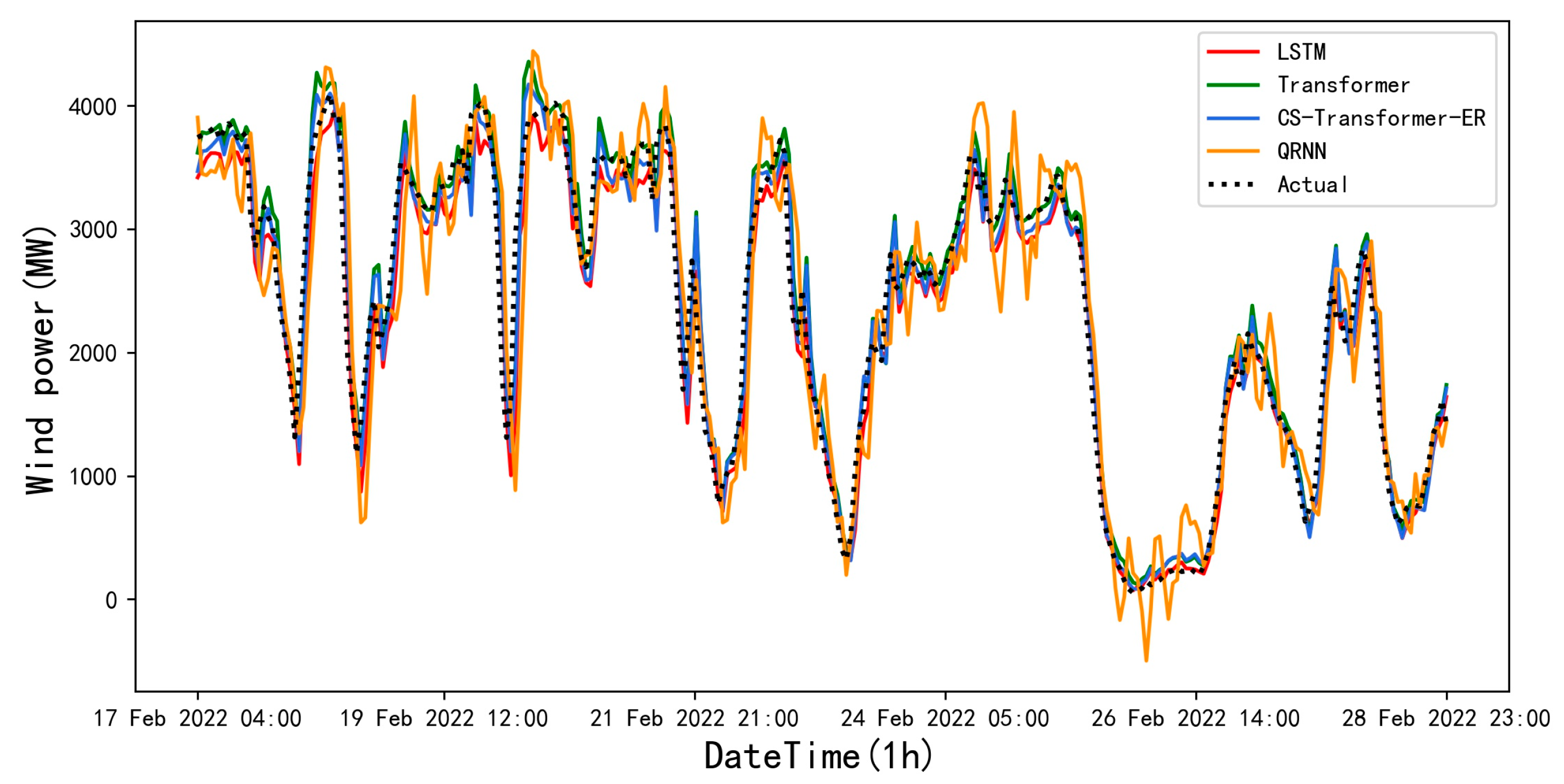
4.2. Comparison of the Model Prediction Results

Nine models are utilized for comparison in order to evaluate the prediction results of classical point estimation methods. These models are appropriately analyzed via four metrics: MAE, RMSE, MAPE, and R2. A comparison of the point prediction results of some of the models is presented in Figure 6. The depicted results indicate that the predicted and actual values for the four models are relatively close. The models exhibit highly accurate prediction performance for intervals where the wind power data are monotonic, while more deviations for intervals are observed for the cases in which the wind power fluctuates and varies. Notably, the QRNN model predicts more dramatic fluctuations between 24 February 2022 and 27 February 2022, which could be related to its training process that utilizes an absolute value loss function. The four error metrics calculated for all models on the test set are given in Table 2.
From the results presented in Table 2, the following conclusions can be drawn:
(1)
Among all the models, the transformer model has the best performance in predicting wind power data. The prediction results of the Transformer-ER model when τ = 0.5 should be theoretically similar to those of the transformer model, and any minor differences between them can be attributed to the numerical calculation variations. In this type of sequential data, compared to the RNN-based model, the transformer model demonstrates superior performance in capturing the internal correlation of longer sequential data. In addition, based on the common sense of deep learning, this effect becomes more noticeable as the amount of training data rises.
(2)
The CS algorithm is effective in searching for hyperparameters of NNMs. Additionally, the achieved results from the CS-Transformer-ER model, which exploits the hyperparameters found through the CS algorithm, also exhibit superior performance in all four evaluation metrics. It is crucial to mention that the low MAPE values for the GRU model could be skewed. The MAPE may not be as reliable as the other three indicators in assessing the prediction performance of the models on the test set due to the presence of intervals in the test set data that contain zero values or close to them. This may lead to the calculated MAPE values tending towards infinity, making the metric unreliable. Furthermore, further optimization of the CS algorithm with more iterations could possibly lead to even better predictions.
(3)
The linear model (i.e., ER) exhibits the worst performance among the benchmark models. Although the MLP and QRNN models are essentially nonlinear, they fail in full consideration of the temporal relationship between data and thus exhibit lower prediction performance than the RNNs. Among the three recurrent neural networks, namely RNN, LSTM, and GRU, the best performance is achieved for the LSTM, which is exploited by most researchers. However, the corresponding MAE error metric of the prediction results is almost 9% higher than that of the transformer model.

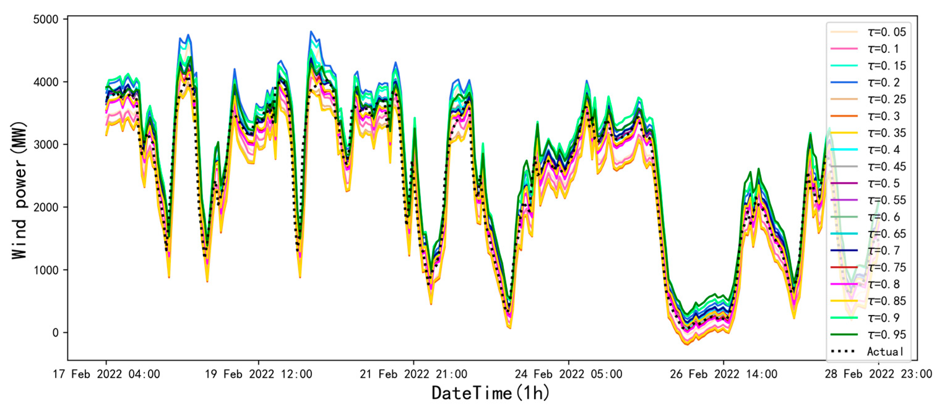
4.3. The Predicted Results Based on the Various Levels of τ

The model has been trained and tested with different levels of τ . The effect of the prediction curve is presented in Figure 7, and the corresponding evaluation metrics calculated are presented in Figure 8.
Figure 7 illustrates the plotted prediction results based on different τ values. It is apparent that the prediction curves are highly similar in trend and degree of fluctuation and are superimposed to configure a confidence interval covering the actual value. It is feasible and reliable to use these predicted values to construct probability density estimation curves.
From Figure 8, it is obtainable that the prediction performance is better and more consistent with less error in the case of τ in the range of 0.4 to 0.85. When the value of τ is considered too large or too small, it leads to a strong asymmetry in the loss function, which is appropriate for describing the corresponding conditional distribution, but the overall prediction performance is poorer.

4.4. Probability Density Prediction Results

Before performing the kernel density estimation, the optimal bandwidth size selected is appropriately verified by a leave-one-out cross-validation for each group of bit data in the test set. The box plots of all optimal bandwidths ( h ) are demonstrated in Figure 9. Figure 9 clearly displays that the majority of the optimal bandwidths ( h ) are in the range of 40–90.
The first nine points of the test set (from 17 February 2022 04:00:00 to 17 February 2022 12:00:00) are chosen, and the actual values and probability density curves of the wind power are demonstrated in Figure 10. The blue curve and the red dashed line represent the kernel density estimation curve and the actual values of the test set, respectively. All the actual values clearly fall within the predicted probability density curve, with the majority of the values being concentrated around the peak of the estimated probability density. This indicates that the estimated probability density effectively captures the inherent uncertainty in wind power generation. The location of the estimated probability density curve peak may be the true value of the wind power data. The probability density estimation offers several advantages such as quantifying uncertainty and improving prediction accuracy, providing decision-makers with more precise information about the WPF.
The results of the probability density estimation for the proposed model, QRNN, and ER are compared in Table 3. The evaluation metrics for the point estimates (i.e., mode, median, and mean) constructed from the probability density estimates of each model are given in this table. Additionally, the corresponding histograms are presented in Figure 11, providing a visual representation of the performance of each model.
The presented results in Table 3 and Figure 11 display that the point prediction errors based on the probability density estimation of the proposed Transformer-ER model are substantially lower in comparison to those of the QRNN and linear ER models, which do not take into account temporal effects. Additionally, regardless of the model or method used, the mode, median, and mean values of the probability density predictions are relatively similar in terms of performance. The mean accuracy is slightly higher than mode and median accuracies because it takes into account all the information of the predicted data. Among all the models and methods, the Transformer-ER model exhibits the lowest MAE and RMSE and the highest R2 for the mean probability density, making it the best point prediction result. Its error metric is smaller than the point prediction results of almost all models in Table 2. It is worth mentioning that the exploitation of the MAPE may not be reliable due to the presence of values close to or equal to zero in the test set.
The evaluation metrics for interval estimation are provided in Table 4. The PICP values of the Transformer-ER, QRNN, and ER models are remarkably different. The QRNN model presents a high PICP, accordingly presenting a low PIEE. The ER of the linear model fails to satisfactorily fit the uncertainty of the wind power data, with a PICP value of only 42.25%. However, the higher PICP of the QRNN is derived from a larger average width of the prediction interval. This means that the QRNN gives an extensive prediction interval, which is of little significance for practical decision making. On the contrary, the Transformer-ER-based model exhibits a more moderate PICP and a smaller PINAW, and its composite index CWC has the smallest value. Therefore, the probability density prediction interval of the Transformer-ER model exhibits higher quality than that of other models.
As can be observed from Figure 12 and Figure 13, while the PIs obtained from the QRNN model cover a majority of the actual values of the wind power, they also exhibit a broader range compared to the PIs from the Transformer-ER model. This broader range of PIs from the QRNN model could lead to a growth of uncertainty in the prediction of wind power forecasting; thus, it could not be beneficial in power planning and decision making. The PIs of the Transformer-ER model are more precise, as they are narrower in zones where the wind power data exhibit a monotonic increase or decrease and broader in zones where the wind power is volatile and variable. This issue would be effectively helpful in capturing the uncertainty in wind power forecasting, providing decision-makers with more relevant and useful information.

5. Conclusions

In the current investigation, a combination of the transformer network that performed best in the sequential data task and expectile regression is proposed for effective wind power prediction via an ERNN structure. The model is optimized by employing the cuckoo search algorithm. The methodology of kernel density estimation is then exploited to achieve the complete probability density curve, which is then built into the point and interval prediction. These predicted results are separately evaluated to provide comprehensive information on the uncertainty of the wind power. The proposed approach is then validated and tested based on the wind power generation data from the Belgian power grid company Elia. The major obtained conclusions are as follows: (1) The proposed model effectively addresses the volatility and stochastic nature of wind power data, provides comprehensive and accurate prediction, reduces the operational risks associated with wind power generation, and enhances the stability of power systems. (2) The transformer network, when compared to the commonly exploited recurrent neural networks, demonstrates the superior capability to capture the internal correlations and dependencies in long sequences and yields a higher level of prediction accuracy. (3) The proposed probability density prediction approach in this paper is capable of providing more comprehensive information for relevant stakeholders and decision-makers and has been proven to be more robust and accurate than point predictions. (4) The proposed ERNN-based model produces more accurate and narrow prediction intervals compared to QRNN models and thereby leads to higher quality prediction intervals in general.

Author Contributions

Conceptualization, X.H.; methodology, H.X. and X.H.; software, H.X.; validation, H.X.; formal analysis, H.X.; investigation, H.X.; resources, H.X.; data curation, H.X.; writing—original draft preparation, H.X.; writing—review and editing, H.X., X.H. and C.L.; visualization, H.X.; supervision, X.H. and C.L.; project administration, X.H.; funding acquisition, X.H. All authors have read and agreed to the published version of the manuscript.

Funding

This research was supported by the National Natural Science Foundation of China (NSFC) (No. 11201356) and Hubei Province Key Laboratory of Systems Science in Metallurgical Process (Wuhan University of Science and Technology) (No. Y202201).

Data Availability Statement

The data presented in this study are available from the following website: https://www.elia.be/en/grid-data/power-generation/wind-power-generation (accessed on 2 January 2023).

Conflicts of Interest

The authors declare no conflict of interest.

References

  1. Tian, C.; Niu, T.; Wei, W. Developing a wind power forecasting system based on deep learning with attention mechanism. Energy 2022, 257, 124750. [Google Scholar] [CrossRef]
  2. He, Y.; Zhang, W. Probability density forecasting of wind power based on multi-core parallel quantile regression neural network. Knowl.-Based Syst. 2020, 209, 106431. [Google Scholar] [CrossRef]
  3. Niu, D.; Sun, L.; Yu, M.; Wang, K. Point and interval forecasting of ultra-short-term wind power based on a data-driven method and hybrid deep learning model. Energy 2022, 124384. [Google Scholar] [CrossRef]
  4. Wang, Y.; Zou, R.; Liu, F.; Zhang, L.; Liu, Q. A review of wind speed and wind power forecasting with deep neural networks. Appl. Energy 2021, 304, 117766. [Google Scholar] [CrossRef]
  5. Qiao, B.; Liu, J.; Wu, P.; Teng, Y. Wind power forecasting based on variational mode decomposition and high-order fuzzy cognitive maps. Appl. Soft Comput. 2022, 129, 109586. [Google Scholar] [CrossRef]
  6. Ding, M.; Zhou, H.; Xie, H.; Wu, M.; Liu, K.-Z.; Nakanishi, Y.; Yokoyama, R. A time series model based on hybrid-kernel least-squares support vector machine for short-term wind power forecasting. ISA Trans. 2021, 108, 58–68. [Google Scholar] [CrossRef]
  7. Liu, K. A random forest-based method for wind power system output power prediction. Light Source Light. 2022, 07, 165–167. [Google Scholar]
  8. Zha, W.; Liu, J.; Li, Y.; Liang, Y. Ultra-short-term power forecast method for the wind farm based on feature selection and temporal convolution network. ISA Trans. 2022, 129, 405–414. [Google Scholar] [CrossRef]
  9. Wang, W.; Liu, H.; Chen, Y.; Zheng, N.; Li, Z.; Ji, X.; Yu, G.; Kang, J. Wind power prediction based on LSTM recurrent neural network. Renew. Energy 2020, 38, 1187–1191. [Google Scholar]
  10. Jin, Y.; Kang, J.; Chen, Y. Wind power prediction technology based on LSTM recurrent neural network algorithm. Electron. Test. 2022, 36, 49–51. [Google Scholar]
  11. Cui, Y.; Chen, Z.; He, Y.; Xiong, X.; Li, F. An algorithm for forecasting day-ahead wind power via novel long short-term memory and wind power ramp events. Energy 2022, 263, 125888. [Google Scholar] [CrossRef]
  12. Ahmad, T.; Zhang, D. A data-driven deep sequence-to-sequence long-short memory method along with a gated recurrent neural network for wind power forecasting. Energy 2022, 239, 122109. [Google Scholar] [CrossRef]
  13. Niu, Z.; Yu, Z.; Tang, W.; Wu, Q.; Reformat, M. Wind power forecasting using attention-based gated recurrent unit network. Energy 2020, 196, 117081. [Google Scholar] [CrossRef]
  14. Li, L.L.; Liu, Z.F.; Tseng, M.L.; Jantarakolica, K.; Lim, M.K. Using enhanced crow search algorithm optimization-extreme learning machine model to forecast short-term wind power. Expert Syst. Appl. 2021, 184, 115579. [Google Scholar] [CrossRef]
  15. Jalali SM, J.; Ahmadian, S.; Khodayar, M.; Khosravi, A.; Shafie-khah, M.; Nahavandi, S.; Catalão, J.P.S. An advanced short-term wind power forecasting framework based on the optimized deep neural network models. Int. J. Electr. Power Energy Syst. 2022, 141, 108143. [Google Scholar] [CrossRef]
  16. Jiang, X.; Xu, Y.; Song, C. A new method for short-term wind power load forecasting. J. Beijing Norm. Univ. 2022, 58, 39–46. [Google Scholar]
  17. Chen, D.; Hong, W.; Zhou, X. Transformer Network for Remaining Useful Life Prediction of Lithium-Ion Batteries. IEEE Access 2022, 10, 19621–19628. [Google Scholar] [CrossRef]
  18. Vaswani, A.; Shazeer, N.; Parmar, N.; Uszkoreit, J.; Jones, L.; Gomez, A.N.; Kaiser, Ł.; Polosukhin, I. Attention is all you need. Adv. Neural Inf. Process. Syst. 2017, 30, 5998–6008. [Google Scholar] [CrossRef]
  19. Wang, L.; He, Y.; Liu, X.; Li, L.; Shao, K. M2TNet: Multi-modal multi-task Transformer network for ultra-short-term wind power multi-step forecasting. Energy Rep. 2022, 8, 7628–7642. [Google Scholar] [CrossRef]
  20. Wu, H.; Meng, K.; Fan, D.; Zhang, Z.; Liu, Q. Multistep short-term wind speed forecasting using transformer. Energy 2022, 261, 125231. [Google Scholar] [CrossRef]
  21. Qu, K.; Si, G.; Shan, Z.; Kong, X.; Yang, X. Short-term forecasting for multiple wind farms based on transformer model. Energy Rep. 2022, 8, 483–490. [Google Scholar] [CrossRef]
  22. Xiong, B.; Lou, L.; Meng, X.; Wang, X.; Ma, H.; Wang, Z. Short-term wind power forecasting based on Attention Mechanism and Deep Learning. Electr. Power Syst. Res. 2022, 206, 107776. [Google Scholar] [CrossRef]
  23. Zhou, X.; Liu, C.; Luo, Y.; Wu, B.; Dong, N.; Xiao, T.; Zhu, H. Wind power forecast based on variational mode decomposition and long short term memory attention network. Energy Rep. 2022, 8, 922–931. [Google Scholar] [CrossRef]
  24. Zhang, J.; Yan, J.; Infield, D.; Liu, Y.; Lien, F. Short-term forecasting and uncertainty analysis of wind turbine power based on long short-term memory network and Gaussian mixture model. Appl. Energy 2019, 241, 229–244. [Google Scholar] [CrossRef] [Green Version]
  25. Zhou, M.; Wang, B.; Guo, S.; Watada, J. Multi-objective prediction intervals for wind power forecast based on deep neural networks. Inf. Sci. 2021, 550, 207–220. [Google Scholar] [CrossRef]
  26. He, Y.; Liu, R.; Li, H.; Wang, S. Short-term power load probability density forecasting method using kernel-based support vector quantile regression and Copula theory. Appl. Energy 2017, 185, 254–266. [Google Scholar]
  27. He, Y.; Li, H. Probability density forecasting of wind power using quantile regression neural network and kernel density estimation. Energy Convers. Manag. 2018, 164, 374–384. [Google Scholar] [CrossRef]
  28. Jiang, C.; Jiang, M.; Xu, Q.; Huang, X. Expectile regression neural network model with applications. Neurocomputing 2017, 247, 73–86. [Google Scholar]
  29. Zhao, H.; Zhang, S.; Zhao, Y.; Liu, H.; Qiu, B. Short-term power load interval forecasting based on adaptive noise-complete empirical modal decomposition-sample entropy-long-term memory neural network and kernel density estimation. Mod. Electr. 2021, 38, 138–146. [Google Scholar]
  30. Li, J.; Zhang, S.; Yang, Z. A wind power forecasting method based on optimized decomposition prediction and error correction. Electr. Power Syst. Res. 2022, 208, 107886. [Google Scholar]
  31. Lu, W.; Duan, J.; Wang, P.; Ma, W.; Fang, S. Short-term Wind Power Forecasting Using the Hybrid Model of Improved Variational Mode Decomposition and Maximum Mixture Correntropy Long Short-term Memory Neural Network. Int. J. Electr. Power Energy Syst. 2023, 144, 108552. [Google Scholar] [CrossRef]
  32. Ewees, A.A.; Al-qaness MA, A.; Abualigah, L.; Elaziz, M.A. HBO-LSTM: Optimized long short term memory with heap-based optimizer for wind power forecasting. Energy Convers. Manag. 2022, 268, 116022. [Google Scholar] [CrossRef]
  33. Dong, Y.; Zhang, H.; Wang, C.; Zhou, X. Wind power forecasting based on stacking ensemble model, decomposition and intelligent optimization algorithm. Neurocomputing 2021, 462, 169–184. [Google Scholar] [CrossRef]
  34. Zhang, Y.; Pi, Z.; Zhu, R.; Song, J.; Shi, J. Wind power prediction based on WOA-BiLSTM neural network. Electrotechnology 2022, 10, 28–31. [Google Scholar]
  35. Kang, H.; Li, Q.; Yu, S.; Yao, S. Ultra-short-term wind power output prediction based on SA-PSO-BP neural network algorithm. Inn. Mong. Power Technol. 2020, 38, 64–68. [Google Scholar]
  36. Yang, X.S.; Deb, S. Cuckoo search via Lévy flights. In Proceedings of the 2009 World Congress on Nature & Biologically Inspired Computing (NaBIC), IEEE, Coimbatore, India, 9–11 December 2009; pp. 210–214. [Google Scholar]
  37. Yang, X.S. Nature-Inspired Metaheuristic Algorithms; Luniver Press: Coventry, UK, 2010; pp. 16–17. [Google Scholar]
Figure 1. Schematic diagram of the multi-head attention.
Electronics 12 01187 g001
Figure 2. Schematic representation of the proposed transformer network.
Electronics 12 01187 g002
Figure 3. The overall flowchart of the cuckoo search algorithm.
Electronics 12 01187 g003
Figure 4. The framework of the overall WPF.
Electronics 12 01187 g004
Figure 5. Wind power plot of aggregate Belgian wind farms from 1 January to 28 February 2022.
Electronics 12 01187 g005
Figure 6. Plots of the point prediction results based on the partial models.
Electronics 12 01187 g006
Figure 7. The graphed prediction results for various levels of τ .
Electronics 12 01187 g007
Figure 8. Prediction metrics for different levels of τ .
Electronics 12 01187 g008
Figure 9. Optimal range of the bandwidth.
Electronics 12 01187 g009
Figure 10. Probability density curves of the wind power for the partial test set.
Electronics 12 01187 g010
Figure 11. Evaluation metrics for point estimates constructed by the probability density prediction.
Electronics 12 01187 g011
Figure 12. Plot of the prediction intervals of the ERNN-based model.
Electronics 12 01187 g012
Figure 13. Plot of the prediction intervals of the QRNN-based model.
Electronics 12 01187 g013
Table 1. The main parameters of the NNMs.
ParameterValue
Number of hidden layers2
Number of neurons in the hidden layer[64, 32]
Batch size32
Maximum number of iterations50
Embedding layer dimension32
Number of multi-head attention heads4
Level τ 0.5
Table 2. Comparison of the point prediction results for all examined models.
ModelMAERMSEMAPER2
ER428.4206565.28591.83110.7672
QRNN354.1195460.96491.82520.8452
LSTM207.8788278.86631.74860.9434
GRU228.8504308.08181.73630.9309
MLP361.4761478.39391.88120.8392
RNN239.0550321.70161.75370.9246
Transformer190.5266269.85001.87870.9470
Transformer-ER194.9061268.88351.79450.9473
CS-Transformer-ER183.9616252.69011.81420.9535
Table 3. The evaluated metrics for point estimation based on several approaches.
MethodsPoint EstimatesMAERMSEMAPER2
Transformer-ERMode203.1176282.00291.90200.9421
Median191.4592271.63751.88430.9463
Mean187.0430263.94771.86110.9493
QRNNMode334.9645428.04051.83010.8665
Median310.3674419.91501.77900.8716
Mean303.6449411.50411.79640.8767
ERMode428.8808564.82081.82740.7676
Median430.2076566.89951.82850.7659
Mean430.0491566.14941.83230.7665
Table 4. Evaluation metrics for the interval prediction of various approaches.
MethodsPICPPIEEPINAWCWC
Transformer-ER0.86970.00640.17280.3510
QRNN0.98240.00080.55800.5580
ER0.42250.05720.17810.4732
Disclaimer/Publisher’s Note: The statements, opinions and data contained in all publications are solely those of the individual author(s) and contributor(s) and not of MDPI and/or the editor(s). MDPI and/or the editor(s) disclaim responsibility for any injury to people or property resulting from any ideas, methods, instructions or products referred to in the content.

