Efficient Reachability Ratio Computation for 2-Hop Labeling Scheme

Abstract

Reachability queries processing has been extensively studied during the past decades. Many approaches have followed the line of designing 2-hop labels to ensure acceleration. Considering its index size cannot be bounded, researchers have proposed to use a part of nodes to construct partial 2-hop labels (p2HLs) to cover as much reachability information as possible. We achieved better query performance using p2HLs with a limited index size and index construction time. However, the adoption of p2HLs was based on intuition, and the number of nodes used to generate p2HLs was fixed in advance blindly, without knowing its applicability. In this paper, we focused on the problem of efficiently computing a reachability ratio (RR) in order to obtain RR-aware p2HLs. Here, RR denoted the ratio of the number of reachable queries that could be answered by p2HLs over the total number of reachable queries involved in a given graph. Based on the RR, users could determine whether p2HLs should be used to answer the reachability queries for a given graph and how many nodes should be chosen to generate p2HLs. We discussed the difficulties of RR computation and propose an incremental-partition algorithm for RR computation. Our rich experimental results showed that our algorithm could efficiently obtain the RR and the overall effects on query performance by different p2HLs. Based on the experimental results, we provide our findings on the use p2HLs for a given graph for processing reachability queries.

1. Introduction

Reachability queries processing is a fundamental graph operation that has been extensively studied in the literature. When given a directed graph, a reachability query $u?⇝v$ inquires whether there exists a directed path from node u to v. It could be used for the Semantic Web, online social networks, biological networks, ontology, transportation networks, etc., to answer whether two nodes have a certain connection. It could also be used as a building block for answering structured queries, such as XQuery (https://www.w3.org/TR/2017/REC-xquery-31-20170321, accessed on 1 January 2020) or SPARQL (https://www.w3.org/TR/rdf-sparql-query, accessed on 1 January 2020). For applications where answering reachability queries is intensively involved, any substantial progress in query time could significantly affect the performance of all applications using it. Over the past decades, researchers have proposed many efficient labeling schemes to facilitate processing reachability queries. According to [1,2], the existing approaches could be classified into two categories: Label-Only and Label+G. Label-Only means that the index conveys the complete reachability information, and the given query $u?⇝v$ could be answered by comparing the labels of u and v, without graph traversal. Label+G means that the index covers partial reachability information, and we may need to perform graph traversal to answer a query.

For Label-Only, the state-of-the-art approaches in [3,4,5] were based on 2-hop labeling schemes [6], and they generated 2-hop labels based on all the nodes to maintain the whole transitive closure (TC). The problem of Label-Only approaches has been that the index size cannot be bounded with respect to the size of the input graph and minimizing the size of the 2-hop labels as NP-hard [6], which makes the index construction a difficult task in practice for dense graphs. For example, it was shown in [2] that when the number of nodes was 10 million and the average degree of the input graph was greater than 6, the state-of-the-art Label-Only approaches, such as TF  [5], DL  [3], and TOL  [4], could not construct the index successfully due to exceeding the memory limit. As compared to Label-Only, the main advantage of Label+G approaches has been that the index could be easily constructed, which meant that Label+G approaches were indispensable when Label-Only approaches were not appropriate for the given graph. Due to that, the index could not cover all the reachability information, and the Label+G approaches usually used two types of labels for pruning in order to terminate the graph traversal in advance. The first was No-Label, which was used to determine whether a query was an unreachable query. The second was Yes-Label, which was used to determine whether a query was a reachable query, including the tree interval [7,8,9] and p2HLs, which were constructed based on a portion of, rather than all of, the nodes. In this paper, we referred to nodes that were used to construct p2HLs as hop-nodes. It was shown in [2] that the state-of-the-art No-Label could correctly answer more than 95% of unreachable queries. However, this was not enough. Although a workload with completely random queries would be heavily skewed towards unreachable queries [9,10], in real scenarios, it would be highly unlikely that most queries would be unreachable, as the node pair in a query would tend to have a certain connection [11]. For Label+G approaches, therefore, processing reachable queries has been regarded as a worst-case scenario due to the need of graph traversal [7], and the query performance has been dominated by the pruning power of Yes-Label when the number of reachable queries increased.

The pruning power of Yes-Label depends on reachability ratio (RR), i.e., the ratio of the number of reachable queries that can be answered by Yes-Label based on the size of the TC. The higher the RR, the larger the probability that the given reachable query can be answered using Yes-Label without graph traversal. Our statistics showed that even using five randomly generated tree intervals, as performed in [10], the RR was less than 10% for most graphs, resulting in poor query performance when the number of reachable queries increased [7]. As a comparison, it was shown in [7] that p2HLs could improve the query performance significantly for many graphs. For example, Figure 1 shows the RR of p2HLs on three graphs, from which we found that even if we constructed p2HLs using 1 hop-node, the RR was greater than 95% on web-uk, meaning the probability that a given reachable query q could be answered by p2HLs was greater than 95% without graph traversal. In practice, however, the RR of p2HLs changed dynamically for different graphs, and the query performance was not as efficient as expected [7]. In shown in Figure 1, the RR was close to 0 on patent, meaning the probability that q could be answered by p2HLs was close to 0. In this case, using p2HLs resulted in only additional costs.

Considering that Label+G approaches are indispensable and its query performance is mainly affected by the pruning power of the most important Yes-Label, i.e., p2HLs, the key problem that needed to be solved was the following: whether we should use p2HLs for a given graph. The answer depended on the RR. For example, given the RR in Figure 1, we could decide to use p2HLs on web-uk but not on patent, as by using the same number of hop-nodes, the RR would be greater than 95% on web-uk and close to 0 on patent. Furthermore, once RR were determined, we could further determine how many hop-nodes should be chosen to construct the p2HLs. For example, according to Figure 1, we could decide to use four hop-nodes for a human, but for web-uk, one hop-node would be sufficient due to its larger RR and smaller index size.

To the best of our knowledge, this was the first work to address RR-aware p2HLs. Computing RR for given p2HLs was not a simple task and, thus, involved two operations. One was computing the size of TC, and the other was computing the exact number of reachable queries that could be answered by p2HLs, which we referred to as the coverage size. Considering that the TC size computation could be efficiently solved by existing methods in [12], the difficulty of RR computation was related to efficiently computing the coverage size. The naive way was by first generating p2HLs based on the selected k-hop-nodes and then obtaining the coverage size by reviewing all the node pairs using p2HLs. In this way, the cost of coverage size computation was $O\left(k\right|V{|}^2)$ and could not be scaled for larger graphs, where V was the set of nodes in the input graph. Furthermore, if the RR was too small to fulfill the requirement, we may need to increase k-value and repeat the above operation, which would then make the RR computation more difficult to solve.

We proposed the computation of the coverage size incrementally, so that when the value of k changed, we could avoid the costly coverage size re-computation to support a more efficient RR computation. The basic concept was, given the coverage size with respect to the k nodes, when we computed the coverage size with respect to $k+1$ hop-nodes, we would not compute it from scratch but only compute the increased coverage size. However, the increased coverage size could not be easily computed. To obtain the increased coverage size with respect to the $(k+1)$th hop-node u, we had to firstly traverse from u to obtain a set of nodes $D_u$ that u could reach, then traverse from u in reverse to obtain the second set of nodes $A_u$ that could reach u. Given $A_u$ and $D_u$, we needed to determine for each pair of nodes $(a,d)$, whether a could reach d and whether that could be determined by the current p2HLs without u, where $a\in A_u,d\in D_u$. If this was possible, we could affirm that a could reach d and whether that could be determined by p2HLs without u and, therefore, should not be considered when computing the increased coverage size with respect to u. The cost of processing one hop-node u was as high as $O\left(k\right|A_u\left|\right|D_u\left|\right)$. Obviously, with an increase in the number of hop-nodes for p2HLs construction, the cost could become unaffordable. For this problem, we proposed dividing both $A_u$ and $D_u$ into a set of disjointed subsets based on an equivalence relationship (as defined later), so that for each pair of subsets $A_1\subseteq A_u$ and $D_1\subseteq D_u$, we only needed to test one reachability query, rather than $|A_1|\times |D_1|$ queries. The cost of the RR computation was, therefore, reduced significantly even when processing large graphs. We made the following contributions.

• To the best of our knowledge, this was the first work to focus on RR-aware p2HLs.
• We proposed a set of algorithms for RR computation. We showed that according to the properties of 2-hop labels, the two sets of nodes that could reach, and be reached by, a certain hop-node could be divided into a set of disjointed subsets, so that the computation cost could be reduced significantly. We proved the correctness and efficiency of our approach.
• We conducted rich experiments on real datasets. The experimental results showed that when compared with the baseline approach, our algorithm operated much more efficiently on RR computations. We also showed the overall query performance was affected by p2HLs with different numbers of hop-nodes, based on which we provided our findings as to whether and how to use p2HLs for a given graph for processing reachability queries.

The remainder of the paper is organized as follows. We discuss the preliminaries and the related work in Section 2. In Section 3, we provide the baseline algorithm for RR computations and propose the first incremental algorithm in Section 4. After that, we propose the optimized incremental algorithm in Section 5. We report our experimental results in Section 6 and conclude our paper in Section 7.

2. Background and Related Work

2.1. Preliminaries

Given a directed graph $\mathcal{G}$, we constructed a directed acyclic graph (DAG) G from $\mathcal{G}$ in linear time [13] by coalescing each strongly connected component (SCC) of $\mathcal{G}$ into a node in G. Then, the reachability query on $\mathcal{G}$ could be answered equivalently on G. We followed the convention and assumed that the input graph was a DAG $G=(V,E)$, where V is the set of nodes and E the set of edges. We defined $i{n}_{}\left(u\right)=\left\{v\right|(v,u)\in E\}$ as the set of in-neighbors of u in G and $ou{t}_{}\left(u\right)=\left\{v\right|(u,v)\in E\}$, the set of out-neighbors of u. We used $u⇝v$ to denote that node u could reach node v in G. The transitive closure (TC) of node u was denoted as $TC\left(u\right)$, which was the set of all nodes that u could reach. The TC size of G was $\left|TC\left(G\right)\right|={\sum }_{u\in V}\left|TC\left(u\right)\right|$. We used $T{C}^{-1}\left(u\right)$ to denote the set of all nodes that could reach u.

Given a set of k nodes $S_k\subseteq V$, we used ${\mathcal{L}}_k$ to denote the 2-hop labels constructed based on the nodes of $S_k$, where each node in $S_k$ was called a hop-node. If $v\in TC\left(u\right)$ and ${\mathcal{L}}_k$ could correctly affirm that $u⇝v$, we assumed ${\mathcal{L}}_k$ (or $S_k$) could cover the reachable query $u⇝v$. Let $N_k$ be the number of distinct reachable queries that are covered by ${\mathcal{L}}_k$, the RR $\alpha$ with respect to $S_k$ is defined as Equation (1).

$$\alpha =N_k/\left|TC\left(G\right)\right|$$

(1)

Problem Statement: 

Given a DAG $G=(V,E)$, its TC size $\left|TC\right(G\left)\right|$, and a hop-node set $S_k\subseteq V$, return the RR of $S_k$.

2.2. Related Work

As no existing works addressed the RR computation, we only discussed existing works on processing reachability queries and the TC size computation.

Label-Only: 

The Label-Only algorithms [3,4,5,6,14] have attempted to compress TC in order to obtain a smaller index size and facilitate answering queries. Recent research includes TF  [5], DL [3], PLL [14], and TOL [4]. The main concept was based on the 2-hop labeling [6] that could answer reachability queries, where each node u was assigned two labels: one of which was an in-label $L_{in}^{}\left(u\right)$, and the other was an out-label $L_{out}^{}\left(u\right)$. The statement $L_{in}^{}\left(u\right)\left(L_{out}^{}\left(u\right)\right)$ consists of a set of nodes v that could reach (and be reached by) u. Based on this labeling scheme, $u?⇝v$ could be answered by computing the result of $L_{out}^{}\left(u\right)\bigcap L_{in}^{}\left(v\right)$. If $L_{out}^{}\left(u\right)\bigcap L_{in}^{}\left(v\right)\ne \varnothing$, then $u⇝v$; otherwise, $u\neg ⇝v$.

Considering that minimizing the 2-hop label size would be NP-hard [6], Cohen et al. proposed a $(log|V\left|\right)$-approximate solution. However, the index construction cost was ${O\left(\right|V\left|\right|E|log(\left|V\right|}^2/\left|E\right|\left)\right)$, which made it difficult to scale for large graphs. Motivated by this, the following works, [3,4,5,14], had to discard the approximation guarantee and focus on finding better ordering strategies to rank nodes in order to improve the efficiency of their 2-hop label construction. In [5], TF folded the given DAG recursively based on the topological level (topo-level). Assuming that all nodes were sorted by certain ranking values, both DL  [3] and PLL  [14] adopted the same concept to compute 2-hop labels that enumerated a node u in each iteration with a forward (backward) breadth-first search (BFS) to add u to an in (or out) label of nodes that u could reach (and could be reached). The TOL [4] framework summarized TF, DL, and PLL and then computed 2-hop labels based on a newly proposed total order.

Recently, researchers proposed computing 2-hop labels in parallel [15,16] to accelerate the construction of 2-hop labels. However, the index size still could not be bounded with respect to the size of the input graph.

Label+G: 

The Label+G methods answered reachability queries using both Yes-Label and No-Label covering partial reachability information. The main advantage, when compared with Label-Only, was that the index size could be bounded. Recent Label+G approaches include those proposed in GRAIL [9,10], FERRARI-G [7], FELINE [8], IP${}^{+}$ [1] and BFL${}^{+}$ [2]. For these approaches, No-Label was used to test whether the given query was an unreachable one, including topo-order [7,8], topo-level [7,8,9], graph interval [7,9,10], i.e., intervals covering all reachable nodes, IP label [1], and Bloom filter label [2]. The Yes-Label was used to test whether the given query was a reachable query, including the tree interval [7,8,9] and p2HLs [7,17].

It was shown by the existing research that No-Label could prune most unreachable queries [2], though the performance of Yes-Label could fluctuate unpredictably [7,17]. Our statistics showed that the RR of the tree interval was usually less than 10%. As a comparison, the RR of p2HLs could be much higher even with very few hop-nodes, as shown by Figure 1. Therefore, adopting p2HLs could improve the query performance of the Label+G approaches significantly for some graphs [7,17]. However, for some other graphs, p2HLs may not work as efficiently as expected [7,17]. Therefore, when considering p2HLs for processing reachability queries, it was necessary that we could quickly obtain the RR to correctly determine whether we should use p2HLs or not, and furthermore, we could then decide the number hop-nodes that should be chosen to construct p2HLs.

Other Reachability Approaches: 

Ref. [18] proposed an index-free approach to process reachability queries on dynamic graphs with an approximate answer. Refs. [19,20] discussed processing label-constrained reachability queries on large graphs. Ref. [21] adopted the concept of 2-hop coverage and proposed an index-based approach to answer span-reachability queries in large temporal graphs.

TC-Size Computation: 

Given a DAG $G=(V,E)$, a path $p=v_0,v_1,...,v_s$ satisfies $\forall i\in [0,s-1]$, $(v_i,v_{i+1})\in E$, where s denotes the length of p. The path decomposition of G is a partition $S_p=\{p_1,p_2,...,p_k\}$, satisfying $V={\bigcup }_{i\in [1,|S_p\left|\right]}{p}_i$ and $\forall i,j\in [1,|S_p\left|\right],i\ne j,p_i\bigcap p_j=\varnothing$. PTR  [22] proposed a linear greedy algorithm to obtain the path partition, based on which [12] proposed an efficient algorithm buTC${}^{+}$ for a TC size computation with time complexity $O\left(r\right|E\left|\right)$, where $r=|S_p|$. This approach processed nodes of each path in a bottom-up method to achieve high efficiency. It was inspired by an observation that for two nodes, u and v, in a path, if $(u,v)\in E$, then $TC\left(v\right)\subset TC\left(u\right)$. Therefore, by processing the nodes of a path in a bottom-up approach with the nodes marked carefully, the nodes in $TC\left(v\right)$ did not need to be revisited when computing $\left|TC\right(u\left)\right|$.

In addition, [4,23,24] proposed estimating the approximate TC size for all nodes in linear time $O\left(\right|V|+|E\left|\right)$.

Note that the TC size computation was different than the TC computation. The former addressed the size of $TC\left(v\right)$, i.e., $\left|TC\right(v\left)\right|$, while the latter returned all nodes in each $TC\left(v\right)$.

3. The Baseline Algorithm

In this section, we first analyze the construction of 2-hop labels and then discuss the RR computation and the baseline algorithm.

Step-1: 2-hop Label Construction. 

To construct 2-hop labels, we followed [3,14] and sorted all nodes by $\left(\right|i{n}_{}\left(u\right)|+1)\times \left(\right|i{n}_{}\left(u\right)|+1)$. The sorting result was $v_1,v_2,...,v_{\left|V\right|}$, where the first node has the largest rank value. We selected the first k nodes to obtain the hop-node set $S_k=\{v_1,v_2,...,v_k\}$. We had the following result: (Equations (2) and (3)).

$$\varnothing =S_0\subset S_1\subset S_2\subset \cdots \subset S_{\left|V\right|}=V$$

(2)

$$S_i\backslash S_{i-1}=\left\{v_i\right\},\mathrm{where}0<i\le \left|V\right|$$

(3)

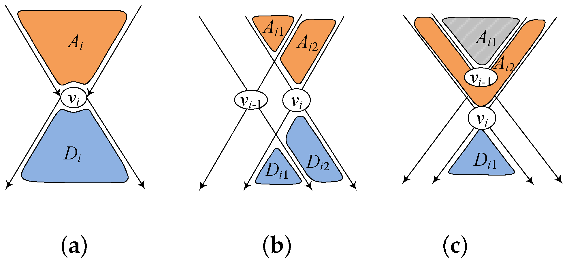
Given $S_i$, the p2HL ${\mathcal{L}}_i$ could be generated by processing $v_i$, based on ${\mathcal{L}}_{i-1}$, according to Equations (2) and (3). Specifically, we performed forward (backward) BFS from $v_i$ to obtain a set $D_i\left(A_i\right)$ of nodes that $v_i$ could reach (could be reached by $v_i$),as denoted by Figure 2a. For each node $a\in A_i$, we added $v_i$ to a’s out-label, i.e., $L_{out}^i\left(a\right)=L_{out}^{i-1}\left(a\right)\cup \left\{v_i\right\}$, denoting that a could reach $v_i$. For each node $d\in D_i$, we added $v_i$ to d’s in-label, i.e., $L_{in}^i\left(d\right)=L_{in}^{i-1}\left(d\right)\cup \left\{v_i\right\}$, denoting that $v_i$ could reach d. After processing $v_i$, we obtained 2-hop labels ${\mathcal{L}}_i$. The superscript i in $L_{out}^i\left(a\right)\left(L_{in}^i\left(a\right)\right)$ denotes that both 2-hop labels $L_{out}^i\left(a\right)$ and $L_{in}^i\left(a\right)$, with respect to node a, are subsets of $S_i$. Here, we could use ${\mathcal{L}}_{i-1}$ to reduce the size of both $A_i$ and $D_i$. For example, in Figure 2c, when processing $v_i$, the backward BFS traversal from $v_i$ could be terminated at $v_{i-1}$, because $v_{i-1}$ reaching $v_i$ could be determined by ${\mathcal{L}}_{i-1}$, and $\forall a\in T{C}^{-1}\left(v_{i-1}\right)$ reaching $v_i$ through $v_{i-1}$ could also be answered by ${\mathcal{L}}_{i-1}$.Therefore, in practice, $A_i\subseteq TC\left(v_i\right)\wedge D_i\subseteq T{C}^{-1}\left(v_i\right)$.

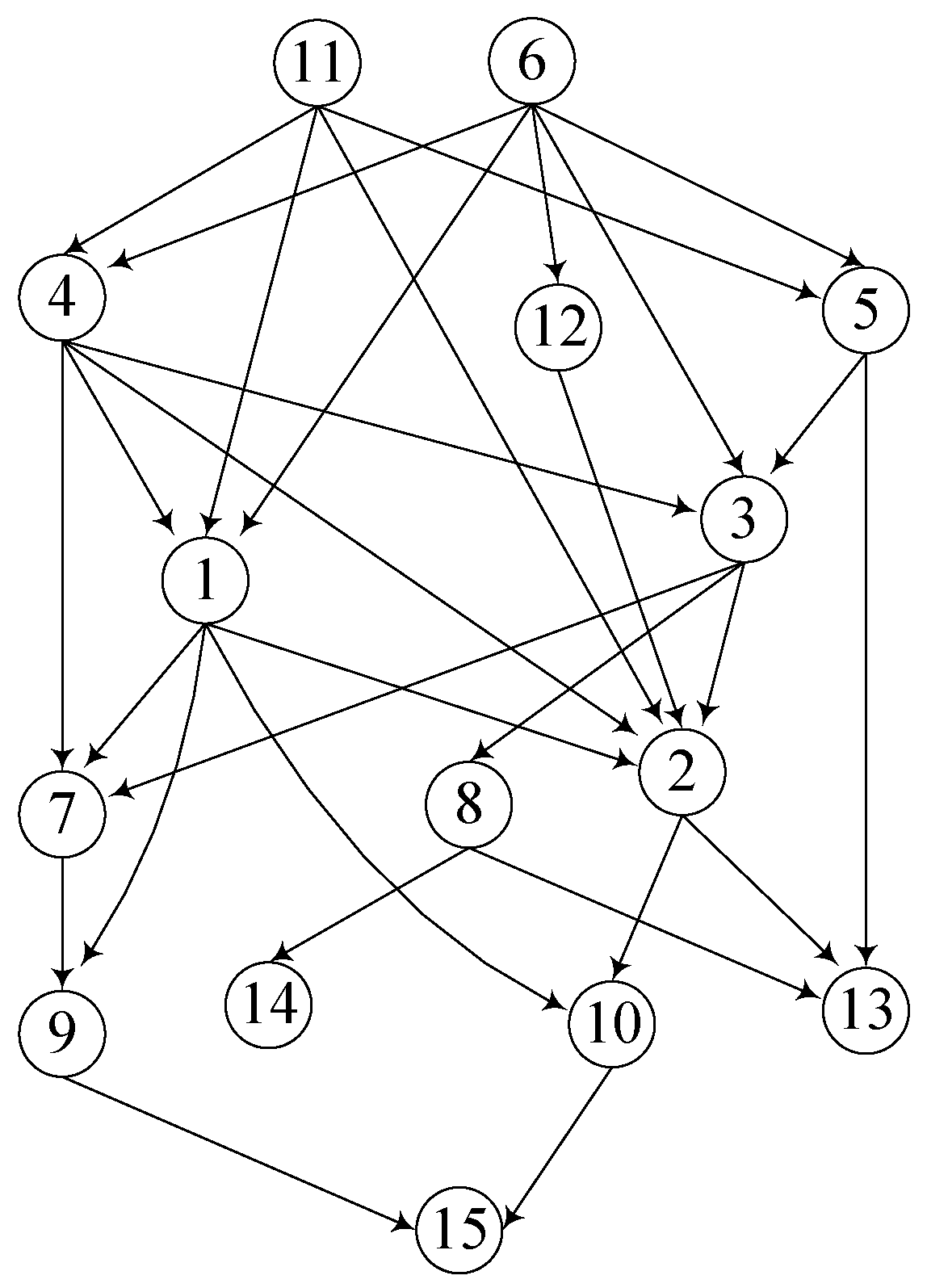
Example 1.

Consider G in Figure 3. Assume that the sorting result is $v_1,v_2,v_3,...,v_{15}$. To obtain ${\mathcal{L}}_2$, we first performed bidirectional BFS of $v_1$ to obtain $A_1=\{v_1,v_4,v_6,v_{11}\}$ and $D_1=\{v_1,v_2,v_7,v_9,v_{10},$$v_{13},v_{15}\}$. After that, we added 1 to the out-label of nodes in $A_1$ and the in-label of nodes in $D_1$, in order to obtain ${\mathcal{L}}_1$. The next processed node was $v_2$. Similarly, we obtained $A_2=\{v_2,v_3,v_5,v_{12}\}$ and $D_2=\{v_2,v_{10},v_{13},v_{15}\}$. Note that all nodes in $A_1$ could reach $v_2$, but some of them were not in $A_2$, because for nodes that were in $A_1$ but not in $A_2$, whether they could reach $v_2$ could be answered by ${\mathcal{L}}_1$. Then, we added 2 to the out- and in-labels of nodes in $A_2$ and $D_2$, as shown by

Table 1. The p2HLs ${\mathcal{L}}_1,{\mathcal{L}}_2,{\mathcal{L}}_3$ constructed based on $S_1=\left\{v_1\right\},S_2=\{v_1,v_2\}$, and $S_3=\{v_1,v_2,v_3\}$, respectively.

Node	${\mathcal{L}}_1$		${\mathcal{L}}_2$		${\mathcal{L}}_3$
	$L_{out}^1\left(v\right)$	$L_{in}^1\left(v\right)$	$L_{out}^2\left(v\right)$	$L_{in}^2\left(v\right)$	$L_{out}^3\left(v\right)$	$L_{in}^3\left(v\right)$
$v_1$	1	1	1	1	1	1
$v_2$		1	2	1, 2	2	1, 2
$v_3$			2		2, 3	3
$v_4$	1		1		1, 3
$v_5$			2		2, 3
$v_6$	1		1		1, 3
$v_7$		1		1		1, 3
$v_8$						3
$v_9$		1		1		1, 3
$v_{10}$		1		1, 2		1, 2
$v_{11}$	1		1		1, 3
$v_{12}$			2		2
$v_{13}$		1		1, 2		1, 2
$v_{14}$						3
$v_{15}$		1		1, 2		1, 2

.

Step-2: RR Computation. 

Given ${\mathcal{L}}_k$ with respect to $S_k$, the baseline approach computed the RR, as follows. First, it obtained the set of nodes that could reach either one of the set of hop-nodes, as shown by Equation (4). Second, it obtained the set of nodes that could be reached by either one of the set of hop-nodes, as shown by Equation (5). It computed the number of reachable queries that could be answered by ${\mathcal{L}}_k$, as shown by Equation (6). Finally, we returned the RR of $S_k$ based on Equation (1).

$$A=\bigcup _{i\in [1,k]}{A}_i$$

(4)

$$D=\bigcup _{i\in [1,k]}{D}_i$$

(5)

$$\begin{array}{cc}\hfill N_k=\left|\right\{(a,d)|& a\in A,d\in D,a\ne d\hfill \\ \hfill & L_{out}^k\left(a\right)\cap L_{in}^k\left(d\right)\ne \varnothing \left\}\right|\hfill \end{array}$$

(6)

Example 2.

Continued example of 1. To compute the RR of $S_2=\{v_1,v_2\}$, we first computed $A_{}=A_1\cup A_2=\{v_1,v_2,v_3,v_4,v_5,v_6,v_{11},v_{12}\}$, $D_{}=D_1\cup D_2=\{v_1,v_2,v_7,v_9,v_{10},v_{13},v_{15}\}$, according to Equations (4) and (5), respectively. Then, we review each pair of nodes $a\in A_{}$ and $d\in D_{}(a\ne d)$ as to whether a reaching d could be answered by ${\mathcal{L}}_2$. Furthermore, we computed the number of answered reachable queries according to Equation (6), which was 42 for G in Figure 3 and ${\mathcal{L}}_2$ in Table 1. Given $TC\left(G\right)=70$, we knew that the RR of $S_2$ was $42/70=60\%$.

The Algorithm: 

The baseline algorithm (Algorithm 1) computed RR in two steps. Step-1 (lines 1–18) first calls the buTC${}^{+}$ algorithm [12] to compute TC size in line 1, and then constructs 2-hop labels ${\mathcal{L}}_k$ and obtained the two sets of nodes, $A_{}$ and $D_{}$. Specifically, it first sorts all nodes in certain order in line 3 and then selects k hop-nodes in line 4. In lines 5–16, it performs forward and backward BFS for each hop-node $v_i$ to construct 2-hop labels ${\mathcal{L}}_i$. During the process, only if the reachability relationship between $v_i$ and the visited node v cannot be answered by 2-hop labels ${\mathcal{L}}_{i-1}$, then it adds $v_i$ to v’s in-label (line 9) or out-label (line 14), and adds v to $D_i$ (line 10) or $A_i$ (line 15); otherwise, it terminates the process because the reachability relationship has already been covered by ${\mathcal{L}}_{i-1}$. In lines 17–18, it obtains the two sets $A_{}$ and $D_{}$ according to Equations (4) and (5). Step-2 (lines 19–21) computes the number of covered reachable queries by ${\mathcal{L}}_k$ according to Equation (6). Finally, it returns the RR in line 22.   

Algorithm 1: blRR$(G,k)$

1 compute $\left|TC\right(G\left)\right|$ by the buTC${}^{+}$ algorithm [12] 2 $N_k\leftarrow 0,S_k\leftarrow \varnothing ,A_{}\leftarrow \varnothing ,D_{}\leftarrow \varnothing$ 3 rank all nodes v in G by $\left(\right|i{n}_{}\left(v\right)|+1)\times \left(\right|i{n}_{}\left(v\right)|+1)$ 4 put the first k nodes into $S_k$ as hop-nodes 5 foreach $(v_i\in S_k)$ do 6    $A_i\leftarrow \varnothing$; $D_i\leftarrow \varnothing$ 7    perform forward BFS from $v_i$, and for each visited v 8       if $(L_{out}^{i-1}\left(v_i\right)\bigcap L_{in}^{i-1}\left(v\right)=\varnothing )$then                  /*${\mathcal{L}}_{i-1}$*/ 9          $L_{in}^i\left(v\right)\leftarrow L_{in}^{i-1}\left(v\right)\bigcup \left\{v_i\right\}$                  /*compute ${\mathcal{L}}_i$*/ 10          $D_i\leftarrow D_i\cup \left\{v\right\}$ 11       else stop expansion from v 12    perform backward BFS from $v_i$, for each visited v 13        if $(L_{out}^{i-1}\left(v\right)\bigcap L_{in}^{i-1}\left(v_i\right)=\varnothing )$then                  /*${\mathcal{L}}_{i-1}$*/ 14           $L_{out}^i\left(v\right)\leftarrow L_{out}^{i-1}\left(v\right)\bigcup \left\{v_i\right\}$                /*compute ${\mathcal{L}}_i$*/ 15          $A_i\leftarrow A_i\cup \left\{v\right\}$ 16        else stop expansion from v 17 $A={\bigcup }_{i\in [1,k]}{A}_i$ 18 $D={\bigcup }_{i\in [1,k]}{D}_i$ 19 foreach $(a\in A_{},d\in D_{},a\ne d)$ do 20    if $(L_{out}^k\left(a\right)\bigcap L_{in}^k\left(d\right)\ne \varnothing )$then                    /*${\mathcal{L}}_k$*/ 21       $N_k\leftarrow N_k+1$ 22 return $\alpha \leftarrow N_k/\left|TC\left(G\right)\right|$ as RR of $S_k$

Analysis: 

The time cost of line 1 was $O\left(r\right|E\left|\right)$ (details are in from Section 2.2) and was $O\left(\right|V\left|\right)$ for line 3 by counting sort. The time cost of BFS from each hop-node $v_i$ was $O\left(\right|V|+|E\left|\right)$ (lines 6–16). During the two BFS traversals, the cost of processing each visited node v was $O\left(k\right)$ (lines 8 and 13). Therefore, the time cost of processing k hop-nodes was $O(k^2\left(\right|V|+\left|E\right|\left)\right)$. As a result, the time cost of Step-1 was $O(k^2\left(\right|V|+\left|E\right|)+r\left|E\right|)$. For Step-2, the time cost of computing $N_k$ was $O\left(k\right|A\left|\right|D\left|\right)$. Therefore, the time complexity of Algorithm 1 was $O(k^2\left(\right|V|+\left|E\right|)+r\left|E\right|+k\left|A\right|\left|D\right|)$.

During the processing, we did not need to actually maintain every $A_i$ and $D_i$; instead, we only needed to maintain $A_{}$ and $D_{}$. Furthermore, we needed to maintain the 2-hop labels with respect to k hop-nodes, so the space cost was $O\left(k\right|V\left|\right)$. As $S_k,A_{}$, and $D_{}$ were bounded by V, the space complexity of Algorithm 1 was $O\left(k\right|V\left|\right)$.

In practice, if the RR was too low to meet the requirement, then we needed to use additional hop-nodes. Therefore, Algorithm 1 would be called once more to compute the new RR, for which all reachability relationships tested for $S_k$ would be tested again for the new hop-node set.

Example 3.

Continue Example 2. Given $A_{}=\{v_1,v_2,v_3,$$v_4,v_5,v_6,v_{11},v_{12}\}$, and $D_{}=\{v_1,v_2,v_7,$$v_9,v_{10},v_{13},v_{15}\}$, we needed to test 56 queries in lines 19–21, due to $|A_{}|=8$ and $|D_{}|=7$. By line 22, we knew the RR was 60%. If the RR was required to be equal or greater than 80%, we would need to enlarge the hop-node set and re-compute the RR from scratch. As a result, the 56 queries tested for $S_2$ would be tested again for the new hop-node set.

4. The Incremental Approach

Considering that Algorithm 1 would be called again when the hop-node set was enlarged, a natural question was: Could we compute the RR incrementally? That is, given the RR with respect to $S_{i-1}$, when we decided to compute it with respect to $S_i=S_{i-1}\cup \left\{v_i\right\}$, we did not start from scratch; instead, we only computed the number of reachable queries that could not be covered by ${\mathcal{L}}_{i-1}$ but could be covered by ${\mathcal{L}}_i$.

However, the increased RR could not be easily computed. On the one hand, by constructing 2-hop labels using hop-node $v_i$, we captured 3 types of reachability relationships: (1) $v_i$ that could reach every node in $D_i\backslash \left\{v_i\right\}$ could be determined by 2-hop labels with respect to $v_i$, and the number of covered reachable queries was $|D_i|-1$; (2) Every node in $A_i\backslash \left\{v_i\right\}$ that could reach $v_i$ could be determined by 2-hop labels with respect to $v_i$, and the number of covered reachable queries was $|A_i|-1$; and (3) each node in $A_i\backslash \left\{v_i\right\}$ that could reach every node in $D_i\backslash \left\{v_i\right\}$ could be determined by 2-hop labels with respect to $v_i$, and the number of covered reachable queries was $\left(\right|A_i|-1)\times \left(\right|D_i|-1)$. Therefore, the number of covered queries by 2-hop labels with respect to $v_i$ was $\left(\right|A_i|-1)\times \left(\right|D_i|-1)+\left(\right|A_i|-1)+\left(\right|D_i|-1)=|A_i|\times |D_i|-1$.

On the other hand, 2-hop labels with respect to different hop-nodes could cover the same reachable queries. For example, consider Figure 2b. After processing $v_{i-1}$, every node $a_1\in A_{i1}$ that could reach every node $d_1\in D_{i1}$ could be covered by 2-hop labels with respect to $v_{i-1}$, because $v_{i-1}\in L_{out}^{i-1}\left(a_1\right)\cap L_{in}^{i-1}\left(d_1\right)$. After processing $v_i$, we knew that $a_1$ could reach $d_1$, which could also be covered by 2-hop labels with respect to $v_i$, because $v_i\in L_{out}^i\left(a_1\right)\cap L_{in}^i\left(d_1\right)$. Then, the increased number of reachable queries with respect to $v_i$ could be computed as Equations (7) and (8), and the total number of reachable queries $N_k$ covered by ${\mathcal{L}}_k$ could be computed as Equation (9).

$$n_i=|A_i|\times |D_i|-1-\lambda$$

(7)

$$\begin{array}{cc}\hfill \lambda =\left|\right\{(a,d)|& a\in A_i,d\in D_i,a\ne d,\hfill \\ \hfill & L_{out}^{i-1}\left(a\right)\cap L_{in}^{i-1}\left(d\right)\ne \varnothing \left\}\right|\hfill \end{array}$$

(8)

$$N_k=\sum _{i\in [1,k]}{n}_i$$

(9)

Therefore, the intuitive approach was to first obtain the two sets of nodes, $A_i$ and $D_i$, and then testing for each pair of nodes $a\in A_i$ and $d\in D_i$, whether a could reach d could be answered by ${\mathcal{L}}_{i-1}$. If the answer was true, then it indicated that $a⇝d$ had already been covered by $S_{i-1}$; otherwise, it was a new covered query and needed to be considered, as shown by Algorithm 2.

In Algorithm 2, we computed the RR for each $S_i$ when $v_i(i\in [1,k])$ had been added into $S_{i-1}$. In lines 15–18, we computed the number of queries that could be covered by ${\mathcal{L}}_{i-1}$. We obtained the increased number of queries in line 19 according to Equation (7). Then, we obtained the RR of $S_i$ in line 21. We computed ${\mathcal{L}}_i$ based on ${\mathcal{L}}_{i-1}$ in lines 22–25. Finally, we returned the RR of $S_k$ in line 26.

Analysis: 

Algorithm 2 computed the two sets $A_i$ and $D_i$ in lines 2–14, and then it computed ${\mathcal{L}}_i$ in lines 22–25. The overall cost of Step-1 was same as that of Algorithm 1, i.e., $O(k^2\left(\right|V|+\left|E\right|)+r\left|E\right|)$. The cost of Step-2 for each hop-node was $O\left(i\right|A_i\left|\right|D_i\left|\right)$. For k hop-node, the cost was $O\left({\sum }_{i\in [1,k]}i\right|A_i\left|\right|D_i\left|\right)$. Therefore, the time complexity of Algorithm 2 was $O(k^2\left(\right|V|+\left|E\right|)+r\left|E\right|+{\sum }_{i\in [1,k]}i|A_i\left|\right|D_i\left|\right)$. Similar to Algorithm 1, the space complexity of Algorithm 2 was $O\left(k\right|V\left|\right)$.

Example 4.

Consider G in Figure 3. Assume that we want to construct p2HLs ${\mathcal{L}}_3$. The first processed node is $v_1$. As $A_1=\{v_1,v_4,v_6,v_{11}\}$, $D_1=\{v_1,v_2,v_7,v_9,v_{10},v_{13},v_{15}\}$, and then we know $N_1=n_1=|A_1|\times |D_1|-1=27$. The second processed node is $v_2$. The p2HLs are shown in Table 1 and $A_2=\{v_2,v_3,v_5,v_{12}\}$, $D_2=\{v_2,v_{10},v_{13},v_{14}\}$. Then, in lines 16–18, we need to test $|A_2|\times |D_2|=16$ queries. As $\lambda =0$, $n_2=|A_2|\times |D_2|-1-0=15$, and $N_2=n_1+n_2=27+15=42$. The third processed node is $v_3$ and $A_3=\{v_3,v_4,v_5,v_6,v_{11}\}$, $D_3=\{v_3,v_7,v_8,v_9,v_{14}\}$. Then, in lines 16–18, we need to test $|A_3|\times |D_3|=25$ queries. As $\lambda =6$, $n_3=|A_3|\times |D_3|-1-6=18$, and $N_3=N_2+n_3=42+18=60$. After processing $v_3$, we had ${\mathcal{L}}_3$, as shown in Table 1, and the RR was $60/70=85.7$% by testing $16+25=41$ queries in Algorithm 2.

As a comparison, for Algorithm 1, $|A_3|=8$, $|D_3|=10$, and we needed to test 80 queries to obtain the RR.

Algorithm 2: incRR$(G,k)$

1 compute $\left|TC\right(G\left)\right|$ by the buTC${}^{+}$ algorithm [12] 2 $N_0\leftarrow 0$ 3 rank all nodes v in G by $\left(\right|i{n}_{}\left(v\right)|+1)\times \left(\right|i{n}_{}\left(v\right)|+1)$ 4 put the first k nodes into $S_k$ as hop-nodes 5 foreach $(v_i\in S_k)$ do 6     $A_i\leftarrow \varnothing ,D_i\leftarrow \varnothing$ 7     perform forward BFS from $v_i$, and for each visited v 8       if $(L_{out}^{i-1}\left(v_i\right)\bigcap L_{in}^{i-1}\left(v\right)=\varnothing )$then                    /*${\mathcal{L}}_{i-1}$*/ 9          $D_i\leftarrow D_i\cup \left\{v\right\}$ 10       else stop expansion from v 11    perform backward BFS from $v_i$, for each visited v 12       if $(L_{out}^{i-1}\left(v\right)\bigcap L_{in}^{i-1}\left(v_i\right)=\varnothing )$then                   /*${\mathcal{L}}_{i-1}$*/ 13          $A_i\leftarrow A_i\cup \left\{v\right\}$ 14       else stop expansion from v 15    $\lambda \leftarrow 0$ 16    foreach $(a\in A_i,d\in D_i,a\ne d)$ do 17       if $(L_{out}^{i-1}\left(a\right)\bigcap L_{in}^{i-1}\left(d\right)\ne \varnothing )$then                   /*${\mathcal{L}}_{i-1}$*/ 18          $\lambda \leftarrow \lambda +1$ 19    $n_i\leftarrow |A_i|\times |D_i|-1-\lambda$ 20    $N_i\leftarrow N_{i-1}+n_i$ 21    $\alpha \leftarrow N_i/\left|TC\left(G\right)\right|$                        /*RR of $S_i$*/ 22    foreach $(a\in A_i)$do                       /*compute ${\mathcal{L}}_i$*/ 23          $L_{out}^i\left(a\right)\leftarrow L_{out}^{i-1}\left(a\right)\bigcup \left\{v_i\right\}$ 24    foreach $(d\in D_i)$do                       /*compute ${\mathcal{L}}_i$*/ 25          $L_{in}^i\left(d\right)\leftarrow L_{in}^{i-1}\left(d\right)\bigcup \left\{v_i\right\}$ 26 return $\alpha$ as RR of $S_k$

5. The Incremental-Partition Approach

5.1. The Equivalence Relationship

Though Algorithm 2 did not need to compute RR from scratch when the hop-node set became large, it still needed to test $|A_i|\times |D_i|$ queries in line 16 with cost $O\left(i\right|A_i\left|\right|D_i\left|\right)$. Given a large hop-node set, the cost could still become unaffordable.

Definition 1. 

[Equivalence Relationship]Given a hop-node $v_i$, its ancestor set was $A_i$, and its descendant set was $D_i$. We assumed the two nodes $a_1,a_2(a_1\ne a_2)$ of $A_i$ were forward-equivalent to each other, denoted as $a_1{\equiv }_F{a}_2$, if they had the same out-labels, i.e., $L_{out}^i\left(a_1\right)=L_{out}^i\left(a_2\right)$. Similarly, the two nodes $d_1,d_2(d_1\ne d_2)$ of $D_i$ were backward-equivalent to each other, denoted as $d_1{\equiv }_B{d}_2$, if they had the same in-label, i.e., $L_{in}^i\left(d_1\right)=L_{in}^i\left(d_2\right)$.

By Definition 1, we could determine that for $A_i$, a partition $\mathcal{A}\left(i\right)=\{A_{i1},A_{i2},...,A_{im}\}$, which consists of a set of m disjointed subsets satisfying that (1) $\forall l,j\in [1,m],l\ne j,A_{il}\cap A_{ij}=\varnothing$ and ${\cup }_{l\in [1,m]}{A}_{il}=A_i$; and (2) $\forall a_l,a_j$ belonging to the same subset, $a_l{\equiv }_F{a}_j$. For $D_i$, we also had a partition $\mathcal{D}\left(i\right)=\{D_{i1},D_{i2},...,D_{in}\}$ satisfying that (1) $\forall l,j\in [1,n],l\ne j,D_{il}\cap D_{ij}=\varnothing$ and ${\cup }_{j\in [1,n]}{D}_{ij}=D_i$; and (2) $\forall d_l,d_j$ belonging to the same subset, $d_l{\equiv }_B{d}_j$. We had the following result.

Theorem 1. 

Given a hop-node $v_i$, its ancestor set $A_i$, and its descendant set $D_i$, the number of tested queries for RR computation was $\left|\mathcal{A}\left(i\right)\right|\times \left|\mathcal{D}\left(i\right)\right|$, which was bounded by $min\left\{\right|A_i|\times |D_i|,4^{i-1}\}$.

Proof. 

Let $\mathcal{A}\left(i\right)\left(\mathcal{D}\left(i\right)\right)$ be the partition of $A_i\left(D_i\right)$ based on the equivalence relationship and ${\mathcal{P}}_A\left(i\right)\left({\mathcal{P}}_D\left(i\right)\right)$ the partition of V with respect to hop-node set $S_i$ and the forward (backward) equivalence relationship. Initially, $\mathcal{A}\left(1\right)=\left\{A_1\right\}(\mathcal{D}\left(1\right)=\left\{D_1\right\})$, ${\mathcal{P}}_A\left(1\right)=\{A_1,V\backslash A_1\}({\mathcal{P}}_D\left(1\right)=\{D_1,V\backslash D_1\})$.

On the one hand, for each subset $A_{il}\in \mathcal{A}\left(i\right)$, the result of testing all the reachability relationships from nodes of $A_{il}$ to any other node was equivalent to each other; thus, we only needed to randomly select a node and let it be the representative node of $A_{il}$ to perform the testing of reachability relationship. Similarly, for each subset $D_{ij}\in \mathcal{D}\left(i\right)$, we could also randomly select a node and let it be the representative node of $D_{ij}$ to test the reachability relationships from any node to the nodes of $D_{ij}$. As a result, the number of tested queries from the nodes of $A_i$ to the nodes of $D_i$ was $\left|\mathcal{A}\left(i\right)\right|\times \left|\mathcal{D}\left(i\right)\right|$. Since $\mathcal{A}\left(i\right)\left(\mathcal{D}\left(i\right)\right)$ was the partition of $A_i\left(D_i\right)$, we knew that $\left|\mathcal{A}\left(i\right)\right|\times \left|\mathcal{D}\left(i\right)\right|\le |A_i|\times |D_i|$.

On the other hand, given the partition ${\mathcal{P}}_A(i-1)\left({\mathcal{P}}_D(i-1)\right)$ of V, the size of ${\mathcal{P}}_A\left(i\right)\left({\mathcal{P}}_D\left(i\right)\right)$ was, at most, twice the size of ${\mathcal{P}}_A(i-1)\left({\mathcal{P}}_D(i-1)\right)$, and all nodes in each subset of ${\mathcal{P}}_A(i-1)\left({\mathcal{P}}_D(i-1)\right)$ could be further divided into, at most, two disjointed subsets. One consisted of nodes that could reach (and be reached by) $v_i$, and the other contained nodes that could reach (or be reached by) $v_i$. Then, the size of ${\mathcal{P}}_A\left(i\right)\left({\mathcal{P}}_D\left(i\right)\right)$ was bounded by $2^i$, and the size of $\mathcal{A}\left(i\right)\left(\mathcal{D}\left(i\right)\right)$ was bounded by $2^{i-1}$. Therefore, the the number of tested reachability queries was bounded by $2^{i-1}\times 2^{i-1}=4^{i-1}$.

Hence, the number of tested queries for RR with respect to hop-node $v_i$ was bounded by $min\left\{\right|A_i|\times |D_i|,4^{i-1}\}$.    □

According to Theorem 1, we could reduce the number of tested reachability queries when processing hop-node $v_i$. As shown by Equation (10), for each pair of subsets $(A_{il}\in \mathcal{A}\left(i\right),D_{ij}\in \mathcal{D}\left(i\right))$, we only needed to review the reachability relationship between their representative nodes $a\in A_{il}$ and $d\in D_{ij}$. To accomplish this, we first determined the partitions of both $A_i$ and $D_i$, according to their equivalence relationship.

$$\lambda =\sum _{\begin{array}{c}a\in A_{il}\in \mathcal{A}\left(i\right)\\ d\in D_{ij}\in \mathcal{D}\left(i\right)\\ L_{out}^{i-1}\left(a\right)\cap L_{in}^{i-1}\left(d\right)\ne \varnothing \end{array}}|A_{il}|\times |D_{ij}|$$

(10)

5.2. Partitions Computation

To obtain the partitions of $A_i$ and $D_i$, the intuitive approach was to sort all nodes in $A_i\left(D_i\right)$ by comparing their out-labels (in-labels) in lexicographic order. After the sorting operation, all equivalent nodes were clustered together. As the size of each label was bounded by i, the cost of computing the partition $\mathcal{A}\left(i\right)\left(\mathcal{D}\left(i\right)\right)$ of $A_i\left(D_i\right)$ was $O(i\times |A_i|\times log|A_i\left|\right)\left(O\right(i\times |D_i|\times log|D_i\left|\right))$.

Let ${\mathcal{P}}_A\left(i\right)$ be the partition of V with respect to hop-node set $S_i$ and the forward equivalence relationship, ${\mathcal{P}}_D\left(i\right)$ the partition of V with respect to $S_i$ and backward equivalence relationship. We obtained the following result.

Theorem 2. 

Assume the hop-node $v_i$ and its ancestor (descendant) set $A_i\left(D_i\right)$ for $\forall v_1,v_2\in A_i\left(D_i\right)$, $v_1{\equiv }_F{v}_2\left(v_1{\equiv }_B{v}_2\right)$, if they belong to the same subset of ${\mathcal{P}}_A(i-1)\left({\mathcal{P}}_D(i-1)\right)$.

Proof. 

We proved this result from two aspects. First, we proved the correctness when both $v_1$ and $v_2$ belonged to $A_i$ (Case-1), and then we proved the correctness when both $v_1$ and $v_2$ belonged to $D_i$ (Case-2).

Case-1 where $v_1,v_2\in A_i$ and $v_i\in L_{out}^i\left(v_1\right)\cap L_{out}^i\left(v_2\right)$.

On the one hand, if $v_1{\equiv }_F{v}_2$, it indicated that $L_{out}^i\left(v_1\right)=L_{out}^i\left(v_2\right)$ according to Definition 1. Hence, $L_{out}^i\left(v_1\right)\backslash \left\{v_i\right\}=L_{out}^i\left(v_2\right)\backslash \left\{v_i\right\}$, i.e., they belonged to the same subset of ${\mathcal{P}}_A(i-1)$.

On the other hand, if both $v_1$ and $v_2$ belonged to the same subset of ${\mathcal{P}}_A(i-1)$, it indicated that before processing hop-node $v_i$, $L_{out}^{i-1}\left(v_1\right)=L_{out}^{i-1}\left(v_2\right)$, according to the definition of ${\mathcal{P}}_A(i-1)$. As $v_1,v_2\in A_i$, we knew that after processing $v_i$, $v_i\in L_{out}^i\left(v_1\right)\cap L_{out}^i\left(v_2\right)$ and $L_{out}^i\left(v_1\right)=L_{out}^i\left(v_2\right)$ still held. According to Definition 1, $v_1{\equiv }_F{v}_2$.

Therefore, we determined that $v_1{\equiv }_F{v}_2$, if they belonged to the same subset of ${\mathcal{P}}_A(i-1)$.

Case-2 where $v_1,v_2\in D_i$ and $v_i\in L_{in}^i\left(v_1\right)\cap L_{in}^i\left(v_2\right)$.

Similar to the proof of Case-1, we knew that $v_1{\equiv }_B{v}_2$, if they belonged to the same subset of ${\mathcal{P}}_D(i-1)$.

Therefore, for $\forall v_1,v_2\in A_i\left(D_i\right)$, $v_1{\equiv }_F{v}_2\left(v_1{\equiv }_B{v}_2\right)$, if they belonged to the same subset of ${\mathcal{P}}_A(i-1)\left({\mathcal{P}}_D(i-1)\right)$.    □

According to Theorem 2, we assigned each node v two set IDs, denoted as $i{d}_A\left(v\right)$ and $i{d}_D\left(v\right)$, which were used to determine which subset it belonged to in ${\mathcal{P}}_A\left(i\right)$ and ${\mathcal{P}}_D\left(i\right)$, respectively. Then, given the ancestor (descendant) set $A_i\left(D_i\right)$ of $v_i$, we only needed to scan all nodes of $A_i\left(D_i\right)$ once to know immediately that for two nodes $v_1$ and $v_2$: If $i{d}_A\left(v_1\right)=i{d}_A\left(v_2\right)(i{d}_D\left(v_1\right)=i{d}_D\left(v_2\right))$ in ${\mathcal{P}}_A(i-1)\left({\mathcal{P}}_D(i-1)\right)$, then $v_1{\equiv }_F{v}_2\left(v_1{\equiv }_B{v}_2\right)$, and definitely belonged to the same subset of ${\mathcal{P}}_A\left(i\right)\left({\mathcal{P}}_D\left(i\right)\right)$. Therefore, ${\mathcal{P}}_A\left(i\right)\left({\mathcal{P}}_D\left(i\right)\right)$ was a refinement of ${\mathcal{P}}_A(i-1)\left({\mathcal{P}}_D(i-1)\right)$, i.e., each element of ${\mathcal{P}}_A\left(i\right)\left({\mathcal{P}}_D\left(i\right)\right)$ was a subset of a unique element of ${\mathcal{P}}_A(i-1)\left({\mathcal{P}}_D(i-1)\right)$.

Recall that when processing the hop-node $v_i$, we first had its ancestor (descendant) set $A_i\left(D_i\right)$ and then obtained the partition $\mathcal{A}\left(i\right)\left(\mathcal{D}\left(i\right)\right)$ of $A_i\left(D_i\right)$, based on the equivalence relationship. Since ${\mathcal{P}}_A\left(i\right)\left({\mathcal{P}}_D\left(i\right)\right)$ was the partition of V with respect to the equivalence relationship, we knew that $\mathcal{A}\left(i\right)\subset {\mathcal{P}}_A\left(i\right)(\mathcal{D}\left(i\right)\subset {\mathcal{P}}_D\left(i\right))$, and the relationship between ${\mathcal{P}}_A\left(i\right)\left({\mathcal{P}}_D\left(i\right)\right)$, ${\mathcal{P}}_A(i-1)\left({\mathcal{P}}_D(i-1)\right)$ and $\mathcal{A}\left(i\right)\left(\mathcal{D}\left(i\right)\right)$ was shown as Equations (11) and (12).

$${\mathcal{P}}_A\left(i\right)=\{P\backslash A_i|P\in {\mathcal{P}}_A(i-1)\}\cup \mathcal{A}\left(i\right)$$

(11)

$${\mathcal{P}}_D\left(i\right)=\{P\backslash D_i|P\in {\mathcal{P}}_D(i-1)\}\cup \mathcal{D}\left(i\right)$$

(12)

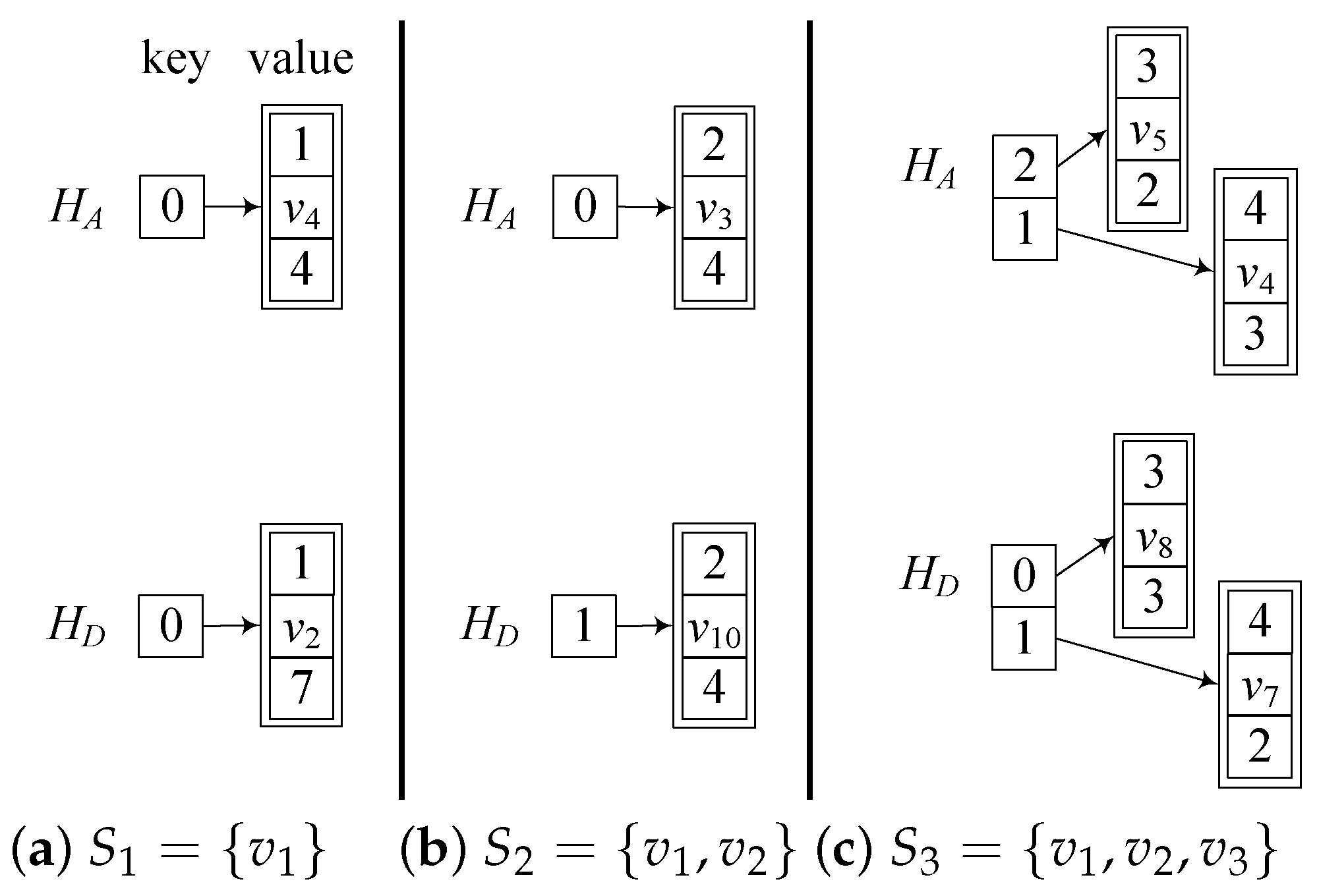
When processing hop-node $v_i$, we used a hash table $H_A^{}\left(H_D^{}\right)$ to achieve linear-time complexity. Each element of $H_A^{}\left(H_D^{}\right)$ was a tuple $(i{d}_o,e_n)$, denoting a subset $A_{il}\left(D_{il}\right)$ of $\mathcal{A}\left(i\right)\left(\mathcal{D}\left(i\right)\right)$, where $i{d}_o$ was, for all nodes of $A_{il}\left(D_{il}\right)$, their old set ID in ${\mathcal{P}}_A(i-1)\left({\mathcal{P}}_D(i-1)\right)$, and $e_n=(i{d}_n,v_1,s)$ was a triple denoting the new set ID for all nodes of $A_{il}\left(D_{il}\right)$, the representative node of $A_{il}\left(D_{il}\right)$, and the size of $A_{il}\left(D_{il}\right)$, respectively.

Example 5.

Consider G in Figure 3. Before processing $v_1$, ${\mathcal{P}}_A\left(0\right)={\mathcal{P}}_D\left(0\right)=\left\{V\right\}$, $\mathcal{A}\left(0\right)=\mathcal{D}\left(0\right)=\varnothing$, and for all nodes v, $i{d}_A\left(v\right)=i{d}_D\left(v\right)=0$.

For the first node $v_1$, we have $A_1=\{v_1,v_4,v_6,v_{11}\}$, $D_1=\{v_1,v_2,v_7,v_9,v_{10},v_{13},v_{15}\}$. Since all nodes in $A_1\left(D_1\right)$ have the same $i{d}_A\left(v\right)\left(i{d}_D\left(v\right)\right)$, we know that $\mathcal{A}\left(1\right)=\left\{A_1\right\}$ and $\mathcal{D}\left(1\right)=\left\{D_1\right\}$. ${\mathcal{P}}_A\left(1\right)=\{A_1,V\backslash A_1\}$, and ${\mathcal{P}}_D\left(1\right)=\{D_1,V\backslash D_1\}$. In

Table 2. The status of set IDs for all nodes.

Node	${\mathit{v}}_1$		${\mathit{v}}_2$		${\mathit{v}}_3$
	${id}_{\mathit{A}}\left(\mathit{v}\right)$	${id}_{\mathit{D}}\left(\mathit{v}\right)$	${id}_{\mathit{A}}\left(\mathit{v}\right)$	${id}_{\mathit{D}}\left(\mathit{v}\right)$	${id}_{\mathit{A}}\left(\mathit{v}\right)$	${id}_{\mathit{D}}\left(\mathit{v}\right)$
$v_1$	1	1	1	1	1	1
$v_2$		1	2	2	2	2
$v_3$			2		3	3
$v_4$	1		1		4
$v_5$			2		3
$v_6$	1		1		4
$v_7$		1		1		4
$v_8$						3
$v_9$		1		1		4
$v_{10}$		1		2		2
$v_{11}$	1		1		4
$v_{12}$			2		2
$v_{13}$		1		2		2
$v_{14}$						3
$v_{15}$		1		2		2

, the two columns under $v_1$ denote ${\mathcal{P}}_A\left(1\right)$ and ${\mathcal{P}}_D\left(1\right)$, where each 1 in the second (third) column correspond to a node in $A_1\left(D_1\right)$. Figure 4a shows the two hash tables denoting $\mathcal{A}\left(1\right)$ and $\mathcal{D}\left(1\right)$, respectively. For $H_A^{}$, there is one (key, value) pair, denoting that $\mathcal{A}\left(1\right)$ contains one subset $A_1$, and for all nodes in $A_1$, their set ID is 0 in ${\mathcal{P}}_A\left(0\right)$. Therefore, they all belong to the same subset in $\mathcal{A}\left(1\right)$, i.e., $\mathcal{A}\left(1\right)=\left\{A_1\right\}$. By $H_A^{}$ in Figure 4a, we know that all nodes in $A_1$ now have the new set ID 1, the representative node of $A_1$ is $v_4$, and $|A_1|=4$.

For the second processed node $v_2$, $A_2=\{v_2,v_3,v_5,v_{12}\}$, $D_2=\{v_2,v_{10},v_{13},v_{14}\}$. As all nodes in $A_2$ have the same set ID 0 in ${\mathcal{P}}_A\left(1\right)$, $\mathcal{A}\left(2\right)=\left\{A_2\right\}$. As shown by Figure 4b, the key is 0, and the triple $(2,v_3,4)$ denotes that the new set ID for all nodes in $A_2$ is 2, the representative node is $v_3$, and $|A_2|=4$. Similarly, all nodes in $D_2$ have the same set ID 1 in ${\mathcal{P}}_D\left(1\right)$, $\mathcal{D}\left(2\right)=\left\{D_2\right\}$, which is denoted as $H_D^{}$ in Figure 4b.

For the third processed node $v_3$, $A_3=\{v_3,v_4,v_5,v_6,v_{11}\}$, $D_3=\{v_3,v_7,v_8,v_9,v_{14}\}$. As $v_3$ and $v_5$ have the same set ID 2 in ${\mathcal{P}}_A\left(2\right)$, they form the subset in $\mathcal{A}\left(3\right)$. Furthermore, $v_4,v_6,v_{11}$ have the same set ID 1 in ${\mathcal{P}}_A\left(2\right)$, they form the second subset in $\mathcal{A}\left(3\right)$. Therefore $\mathcal{A}\left(3\right)=\{\{v_3,v_5\},\{v_4,v_6,v_{11}\}\}$. Similarly, $\mathcal{D}\left(3\right)=\{\{v_3,v_8,v_{14}\},\{v_7,v_9\}\}$. Both $\mathcal{A}\left(3\right)$ and $\mathcal{D}\left(3\right)$ are denoted by $H_A^{}$ and $H_D^{}$ in Figure 4c, respectively.

The Algorithm: 

As shown by Algorithm 3, for each hop-node $v_i$, we first performed forward and backward BFS to obtain $D_i$ (lines 6–15) and $A_i$ (lines 16–25). At the same time, we generated their partitions $\mathcal{D}\left(i\right)$ and $\mathcal{A}\left(i\right)$, for which each subset was recorded in $H_D^{}$ and $H_A^{}$, respectively. In lines 26–29, we computed $\lambda$ according to Equation (10), which was the number of reachable queries that were covered by ${\mathcal{L}}_{i-1}$. In line 30, we obtained the number of reachable queries that could be covered by ${\mathcal{L}}_i$ but not by ${\mathcal{L}}_{i-1}$. After that, we had the total number of covered reachable queries in line 31 and the RR in line 33. Finally, we generated ${\mathcal{L}}_i$ in lines 34–37 and returned the RR of $S_k$ in line 38.

It was worth noting that for Algorithm 3, the improvements was related to not only the coverage size computation, but also the TC size computation. In line 32, we obtained an estimated TC size by the approach in [23], which operated in linear time $O\left(\right|V|+|E\left|\right)$ and was more efficient than the exact approach in [12]. Since the denominator in Equation (1) did not change for ${\alpha }_i(i\in [1,k])$, we could achieve the same effect using an approximate TC size for the RR computation.

Algorithm 3: incRR${}^{+}(G=(V,E),k,TC\left(G\right))$

1 $N_0\leftarrow 0$; $n_A\leftarrow 0$; $n_D\leftarrow 0$; 2 rank all nodes v in G by $\left(\right|i{n}_{}\left(v\right)|+1)\times \left(\right|i{n}_{}\left(v\right)|+1)$ 3 put the first k nodes into $S_k$ as hop-nodes 4 foreach $(v_i\in S_k)$ do 5     $A_i\leftarrow \varnothing$; $D_i\leftarrow \varnothing$; $H_A^{}\leftarrow \varnothing$; $H_D^{}\leftarrow \varnothing$ 6     perform forward BFS from $v_i$, and for each visited v 7       if $(L_{out}^{i-1}\left(v_i\right)\bigcap L_{in}^{i-1}\left(v\right)=\varnothing )$then                   /*${\mathcal{L}}_{i-1}$*/ 8          if $(i{d}_A\left(v\right)\notin H_D^{})$ then 9             $n_A\leftarrow n_A+1$ 10             $H_D^{}\left[i{d}_A\left(v\right)\right]\leftarrow (n_A,v,1)$ 11          else 12             $H_D^{}\left[i{d}_A\left(v\right)\right].s\leftarrow H_D^{}\left[i{d}_A\left(v\right)\right].s+1$ 13          $D_i\leftarrow D_i\cup \left\{v\right\}$ 14          $i{d}_A\left(v\right)\leftarrow n_A$ 15       else stop expansion from v 16    perform backward BFS from $v_i$, for each visited v 17       if $(L_{out}^{i-1}\left(v\right)\bigcap L_{in}^{i-1}\left(v_i\right)=\varnothing )$then                  /*${\mathcal{L}}_{i-1}$*/ 18          if $(i{d}_D\left(v\right)\notin H_A^{})$ then 19             $n_D\leftarrow n_D+1$ 20             $H_A^{}\left[i{d}_D\left(v\right)\right]\leftarrow (n_D,v,1)$ 21          else 22             $H_A^{}\left[i{d}_D\left(v\right)\right].s\leftarrow H_A^{}\left[i{d}_D\left(v\right)\right].s+1$ 23          $A_i\leftarrow A_i\cup \left\{v\right\}$ 24          $i{d}_D\left(v\right)\leftarrow n_D$ 25    else stop expansion from v 26    $\lambda \leftarrow 0$ 27    foreach $((id,a,s_A)\in H_A^{},(id,d,s_D)\in H_A^{})$ do 28       if $(L_{out}^{i-1}\left(a\right)\bigcap L_{in}^{i-1}\left(d\right)\ne \varnothing )$then                  /*${\mathcal{L}}_{i-1}$*/ 29          $\lambda \leftarrow \lambda +|s_A|\times |s_D|$ 30    $n_i\leftarrow |A_i|\times |D_i|-1-\lambda$ 31    $N_i\leftarrow N_{i-1}+n_i$ 32    estimate the TC size by Formula 3 in [23] 33    $\alpha \leftarrow N_i/\left|TC\left(G\right)\right|$                        /*RR of $S_i$*/ 34    foreach $(a\in A_i)$do                      /*compute ${\mathcal{L}}_i$*/ 35       $L_{out}^i\left(a\right)\leftarrow L_{out}^{i-1}\left(a\right)\bigcup \left\{v_i\right\}$ 36    foreach $(d\in D_i)$do                      /*compute ${\mathcal{L}}_i$*/ 37       $L_{in}^i\left(d\right)\leftarrow L_{in}^{i-1}\left(d\right)\bigcup \left\{v_i\right\}$ 38 return $\alpha$ as RR of $S_k$

Example 6.

Consider G in Figure 3. Assume that we want to compute the RR of $S_3=\{v_1,v_2,v_3\}$.

For $v_1$, as there is no covered reachability relationship, we do not need to test any queries in lines 28. As $|A_1|=4$, $|D_1|=7$, $n_1=|A_1|\times |D_1|-1=27$ in line 30 of Algorithm 3.

For $v_2$, as both $\left|\mathcal{A}\left(2\right)\right|=\left|\mathcal{D}\left(2\right)\right|=1$, we only need to test one reachable query, i.e., whether $v_3?⇝v_{10}$ can be answered by ${\mathcal{L}}_1$. As $L_{out}^1\left(v_3\right)\cap L_{in}^1\left(v_{10}\right)=\varnothing$, we know that $n_2=|A_2|\times |D_2|-1=15$ in line 30 of Algorithm 3.

For $v_3$, as shown by Figure 4c, we know that $\mathcal{A}\left(3\right)=\{\{v_3,v_5\},\{v_4,v_6,v_{11}\}\}$ and $\mathcal{D}\left(3\right)=\{\{v_3,v_8,v_{14}\},\{v_7,v_9\}\}$. In line 28, we only need to test $\left|\mathcal{A}\left(3\right)\right|\times \left|\mathcal{D}\left(3\right)\right|=2\times 2=4$ reachable queries. As whether $v_4$ can reach $v_7$ can be answered by ${\mathcal{L}}_2$, we know that whether all nodes in $\{v_4,v_6,v_{11}\}$ can reach every node in $\{v_7,v_9\}$ can be answered by ${\mathcal{L}}_2$; thus, $\lambda =6$ for $v_3$. In line 30, we know that $n_3=|A_3|\times |D_3|-1-\lambda =5\times 5-1-6=18$.

Then, we know $N_3=n_1+n_2+n_3=27+15+18=60$, and the RR is $\alpha =N_3/\left|TC\left(G\right)\right|=60/70=85.7$%. During the process, the total number of tested reachability queries by Algorithm 3 was.

As a comparison, the total number of tested queries for Algorithm 2 was 41, and is 80 for Algorithm 1 to obtain the RR.

Analysis: 

As Algorithm 3 computed the approximate TC size in linear time, the time cost of Step-1 was $O(k^2\left(\right|V|+\left|E\right|)$. The difference was found in Step-2. The cost of Step-2 for each hop-node was $O\left(i\right|\mathcal{A}\left(i\right)\left|\right|\mathcal{D}\left(i\right)\left|\right)$. For k hop-nodes, the cost was $O\left({\sum }_{i\in [1,k]}i\right|\mathcal{A}\left(i\right)\left|\right|\mathcal{D}\left(i\right)\left|\right)$ for coverage computation. The time complexity of Algorithm 3 was, therefore, $O(k^2\left(\right|V|+\left|E\right|)+{\sum }_{i\in [1,k]}i\left|\mathcal{A}\left(i\right)\right|\left|\mathcal{D}\left(i\right)\right|)$. The space complexity of Algorithm 3 was $O\left(k\right|V\left|\right)$.

6. Experiment

In this section, we show the experimental results of the RR computation. The baseline algorithms included blRR, incRR, and incRR${}^{+}$. Moreover, we show the impacts of p2HLs on processing reachability queries based on the state-of-the-art algorithm FL [8] and BFL${}^{+}$ [2], in terms of index size, index construction time, and query time. We implemented all algorithms using C++ and compiled them using G++ 6.2.0. All experiments were conducted on a desktop computer with an Intel(R) Core(TM) i5-1135G7 @ 2.4 GHz CPU, 16 GB memory, and Ubuntu 18.04.1 Linux OS. For algorithms that processed $\ge 3$ h or exceed the memory limit (16GB), we indicated their results as “–” in the tables.

Datasets: 

Table 3. Statistics of datasets, where $d=2\left|E\right|/\left|V\right|$ is the average degree of G, $\left|TC\right(·\left)\right|$ is the average number of reachable nodes for nodes of G, and $n_t$ is the number of topological levels (the length of the longest path) of G.

Dataset	$\left|\mathit{V}\right|$	$\left|\mathit{E}\right|$	d	$\left|\mathit{T}\mathit{C}\right(·\left)\right|$	${\mathit{n}}_{\mathit{t}}$
human	38,811	39,576	2.04	9	18
anthra	12,499	13,104	2.10	12	16
agrocyc	12,684	13,408	2.11	13	16
ecoo	12,620	13,350	2.12	14	22
vchocyc	9491	10,143	2.14	14	21
arxiv	6000	66,707	22.24	928	167
email	231,000	223,004	1.93	11,698	7
LJ	971,232	1,024,140	2.11	206,907	24
web	371,764	517,805	2.79	55,055	34
10cit-Patent	1,097,775	1,651,894	3.01	3	7
10citeseerx	770,539	1,501,126	3.90	70	36
05cit-Patent	1,671,488	3,303,789	3.95	8	12
05citeseerx	1,457,057	3,002,252	4.12	116	36
citeseerx	6,540,401	15,011,260	4.59	15,510	59
dbpedia	3,365,623	7,989,191	4.75	83,659	146
patent	3,774,768	16,518,947	8.75	1544	32
twitter	18,121,168	18,359,487	2.03	1,346,820	22
web-uk	22,753,644	38,184,039	3.36	3,417,930	2793

shows the statistics of 18 real datasets, where the first 6 were small datasets (|V| ≤ 100,000) downloaded from the same web page (https://code.google.com/archive/p/grail/downloads, accessed on 1 January 2020). The following 12 datasets were large (|V| > 100,000). These datasets have usually been used in the recent works for processing reachability queries [1,2,3,4,5,7,8,9,14,23]. Among these datasets, human, anthra, agrocyc, ecoo, and vchocyc were graphs describing the genome and biochemical machinery of E. coli K-12 MG1655. The site (http://snap.stanford.edu/data/index.html, accessed on 1 January 2020) is an email network. LJ is an online social network soc-LiveJournal1 (http://snap.stanford.edu/data/index.html, accessed on 1 January 2020). The source web is a web graph web-Google (https://code.google.com/p/ferrari-index/downloads/list, accessed on). In addition, arxiv, 10cit-Patent (http://pan.baidu.com/s/1bpHkFJx, accessed on 1 January 2020), 10citeseerx (http://pan.baidu.com/s/1bpHkFJx, accessed on 1 January 2020), 05cit-Patent (http://pan.baidu.com/s/1bpHkFJx, accessed on 1 January 2020), 05citeseerx (http://pan.baidu.com/s/1bpHkFJx, accessed on 1 January 2020), citeseerx (https://code.google.com/archive/p/grail/downloads, accessed on 1 January 2020), and patent (https://code.google.com/archive/p/grail/downloads, accessed on 1 January 2020) (cit-Patents) are all citation networks. The source dbpedia (http://pan.baidu.com/s/1c00Jq5E, accessed on 1 January 2020) is a knowledge graph Dbpedia. The sourcetwitter (https://code.google.com/p/ferrari-index/downloads/list, accessed on 1 January 2020) is a DAG transformed from a large-scale social network with 55 million users and 1.96 billion edges [25]. The source web-uk (https://code.google.com/p/ferrari-index/downloads/list, accessed on 1 January 2020) is a DAG transformed from a web graph dataset with 133 million nodes and 5.5 billion edges. The statistics in Table 3 are that of the DAGs.

6.1. RR Computation

RR and Index Size: 

We show RR and the index size ratio (ISR) of these datasets in Figure 5, where ISR denotes the ratio of the size of p2HLs over the size of the 2-hop labels, with respect to all nodes. From Figure 5, we observed the following.

First, all datasets could be classified into three categories according to their RRs. The first (D1) included email, LJ, web, citeseerx, dbpedia, twitter, and web-uk, for which the RR was more than 99%, even when $k=1$, and both the RR and ISR do not significantly change with the increase in k. The second type (D2) included human, anthra, agrocyc, ecoo, vchocyc, and arxiv, for which both the RR and ISR increased with the increase in k. The third type (D3) included 10cit-Patent, 10citeseerx, 05cit-Patent, 05citeseerx, and patent, for which both the RR and ISR were very small or even approach zero, and with the increase in k, both RR and ISR did not significantly change.The value of k, therefore, only affected the second type of dataset, and the RR was more than 80% when $k\ge 16$ for all datasets of the second type, which indicated that this approach could benefit from using p2HLs on datasets of both the first and second types.

Second, the storage space used to maintain p2HLs was small, when compared with the RR value. For example, for the first type of dataset, we used about $1/4$ of the available storage space (ISR $\approx 25$%) to maintain more than 99% (RR $>99$%) of the reachability information.

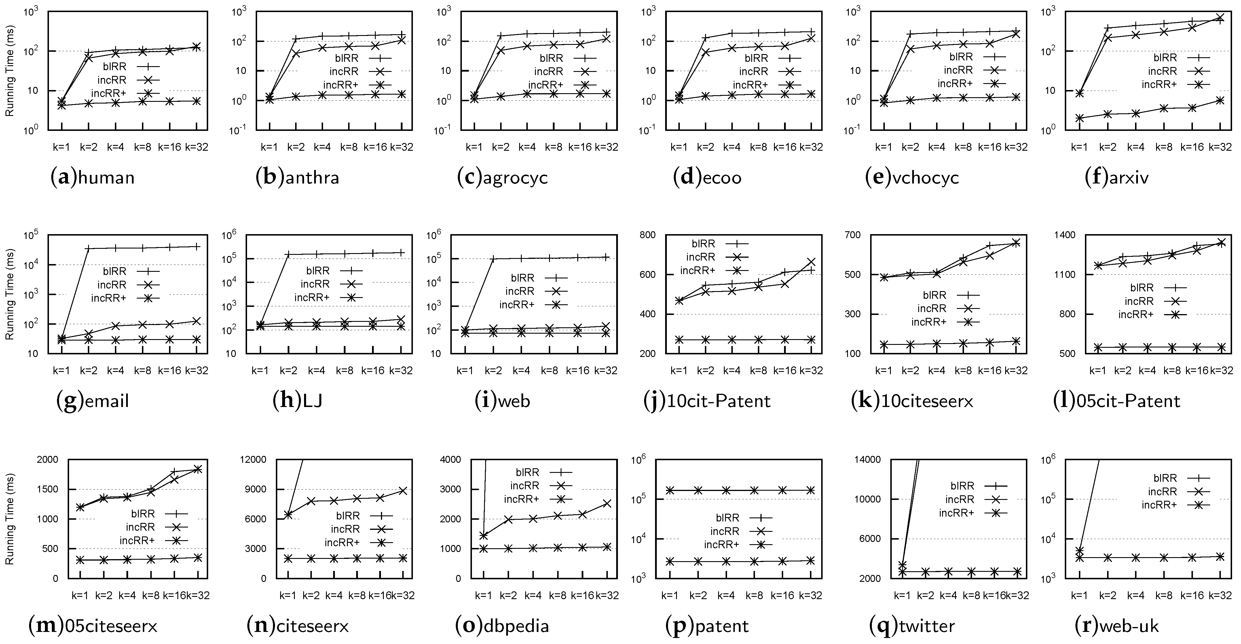
Operational Time: 

Figure 6 shows the comparison of the operational time for the RR computation, from which we knew that incRR${}^{+}$ was much faster than both blRR and incRR, on all datasets, and incRR operated faster than blRR on most datasets. For example, incRR${}^{+}$ was faster than blRR by more than two or three orders of magnitude on most datasets, and incRR was ten-times faster than blRR on email, LJ, web, citeseerx, and dbpedia. According to the last to the second column of Table 3, the average number of reachable nodes was usually high. Therefore, the number of tested reachability queries by blRR was significantly high. Although incRR could reduce the number of tested reachability queries, it still needed to test significantly more reachability queries than incRR${}^{+}$. Neither blRR nor incRR could obtain the value of the RR on both twitter and web-uk for $k\ge 2$ in a limited time frame (3 h), due to testing too many reachability queries.

Based on the above results, we knew that our incRR${}^{+}$ algorithm could be used to efficiently compute the RR for a given dataset, which allowed us to determine whether we could use p2HLs to facilitate processing reachability queries.

6.2. Processing Reachability Queries

We combined p2HLs with FELINE [8] (abbr. FL) and BFL${}^{+}$ [2] to show the impact of p2HLs on processing reachability queries in

Table 4. Comparison of the index size (MB).

Dataset	FL-0	FL-16	FL-32	FL-64	FL-128	BFL${}^{+}$-0	BFL${}^{+}$-16	BFL${}^{+}$-32	BFL${}^{+}$-64	BFL${}^{+}$-128
human	0.74	0.89	1.04	1.33	1.92	1.09	1.23	1.38	1.68	2.27
anthra	0.24	0.29	0.33	0.43	0.62	0.36	0.41	0.45	0.55	0.74
agrocyc	0.24	0.29	0.34	0.43	0.63	0.36	0.41	0.46	0.56	0.75
ecoo	0.24	0.29	0.34	0.43	0.62	0.36	0.41	0.46	0.56	0.75
vchocyc	0.18	0.22	0.25	0.32	0.47	0.27	0.31	0.35	0.42	0.56
arxiv	0.11	0.14	0.16	0.20	0.30	0.25	0.27	0.29	0.34	0.43
email	4.41	5.29	6.17	7.93	11.45	6.39	7.27	8.15	9.92	13.44
LJ	18.52	22.23	25.93	33.34	48.16	27.26	30.96	34.67	42.08	56.90
web	7.09	8.51	9.93	12.76	18.43	11.52	12.94	14.35	17.19	22.86
10cit-Patent	20.94	25.13	29.31	37.69	54.44	32.16	36.35	40.54	48.91	65.66
10citeseerx	14.70	17.64	20.58	26.45	38.21	22.34	25.28	28.22	34.10	45.85
05cit-Patent	31.88	38.26	44.63	57.38	82.89	51.56	57.94	64.32	77.07	102.57
05citeseerx	27.79	33.35	38.91	50.02	72.25	42.11	47.67	53.23	64.35	86.58
citeseerx	124.75	149.70	174.65	224.55	324.34	185.10	210.05	235.00	284.90	384.70
dbpedia	64.19	77.03	89.87	115.55	166.90	109.16	122.00	134.84	160.52	211.87
patent	72.00	86.40	100.80	129.60	187.19	132.91	147.31	161.71	190.51	248.11
twitter	345.63	414.76	483.89	622.14	898.65	475.78	544.91	614.03	752.29	1028.79
web-uk	433.99	520.79	607.59	781.18	1128.38	654.25	741.05	827.84	1001.44	1348.63

,

Table 5. Comparison of the index construction time (ms).

Dataset	FL-0	FL-16	FL-32	FL-64	FL-128	BFL${}^{+}$-0	BFL${}^{+}$-16	BFL${}^{+}$-32	BFL${}^{+}$-64	BFL${}^{+}$-128
human	9.01	11.63	13.12	13.27	13.29	0.92	3.52	3.64	4.47	4.54
anthra	2.89	3.53	4.20	4.26	4.39	0.31	1.08	1.16	1.18	1.21
agrocyc	2.96	3.80	4.15	4.72	4.48	0.25	1.11	1.21	1.26	1.47
ecoo	3.08	3.78	4.42	6.56	4.51	0.25	1.11	1.24	1.31	1.61
vchocyc	2.22	2.79	3.58	3.89	4.07	0.21	0.86	0.89	0.93	0.99
arxiv	4.71	5.93	7.65	8.57	9.76	1.05	3.45	3.66	4.32	5.00
email	81.3	87.9	101.8	97.2	97.9	8.7	27.6	27.9	29.8	30.4
LJ	325.1	381.7	438.3	430.7	442.2	43.5	135.7	138.1	138.3	139.0
web	178.5	215.8	241.7	240.6	245.5	33.2	90.2	93.4	91.2	96.5
10cit-Patent	801.3	1026.2	1084.9	1055.0	1085.0	189.4	448.9	451.7	454.2	466.7
10citeseerx	376.3	497.7	527.9	531.4	550.0	90.2	233.7	236.4	243.0	248.6
05cit-Patent	1517.8	1966.1	1989.4	2037.9	2048.2	417.8	937.8	954.9	975.9	974.0
05citeseerx	775.6	1032.4	1087.6	1076.4	1146.7	197.5	509.2	517.3	525.6	552.4
citeseerx	4063.9	5615.0	6061.8	6002.4	6123.3	1371.5	3179.8	3182.9	3221.6	3234.7
dbpedia	2264.3	2982.4	3200.0	3218.6	3209.9	595.8	1391.9	1396.7	1410.9	1436.2
patent	5022.8	7642.4	7818.6	7890.3	7862.5	2266.9	4725.9	4786.5	4833.9	4984.7
twitter	6287.6	7497.8	8287.8	8285.5	8770.7	1014.2	2760.4	2761.9	2791.2	2812.9
web-uk	8689.7	9968.6	11,138.9	11,185.5	11,559.9	1116.6	3204.8	3236.5	3374.6	3375.9

and

Table 6. Comparison of the query time (ms).

Dataset	FL-0	FL-16	FL-32	FL-64	FL-128	BFL${}^{+}$-0	BFL${}^{+}$-16	BFL${}^{+}$-32	BFL${}^{+}$-64	BFL${}^{+}$-128
human	24.6	4.4	4.1	4.4	5.0	15.5	7.9	8.5	8.4	10.1
anthra	26.2	5.4	4.6	5.0	5.3	13.3	6.8	6.9	6.9	7.5
agrocyc	24.5	5.5	5.3	5.0	5.6	16.3	7.7	7.5	6.9	8.2
ecoo	28.0	5.7	5.1	5.4	5.6	13.4	7.2	7.1	7.2	7.6
vchocyc	26.9	5.0	4.8	4.8	5.5	13.3	6.9	7.7	7.0	7.5
arxiv	479.1	153.4	144.2	140.7	140.3	177.4	37.3	36.3	35.6	32.6
email	82.2	12.4	13.2	13.9	20.5	47.6	23.9	23.0	23.4	27.7
LJ	108.7	27.7	25.0	27.4	33.5	58.0	31.9	30.7	34.5	37.9
web	142.9	34.2	31.7	34.9	41.0	76.5	32.7	32.3	33.3	37.0
10cit-Patent	155.8	169.2	175.0	189.2	196.4	96.2	112.7	135.3	147.1	145.4
10citeseerx	206.2	190.3	182.7	177.3	188.9	113.2	114.7	115.0	113.8	117.8
05cit-Patent	410.4	381.2	367.2	352.3	363.7	197.5	199.3	192.0	185.7	184.7
05citeseerx	250.8	218.8	217.2	207.0	220.1	130.9	136.1	131.2	130.3	138.1
citeseerx	2207.8	76.3	73.5	77.4	85.7	988.1	64.2	67.4	67.1	73.7
dbpedia	346.6	55.8	54.8	57.6	62.5	205.0	49.0	49.3	48.8	52.6
patent	13,716.5	12,584.4	12,629.1	12,026.3	12,021.3	3415.1	3388.7	3248.2	3204.3	3114.2
twitter	168.9	42.8	43.0	47.8	54.5	113.0	64.9	64.2	72.6	83.0
web-uk	256.9	115.0	127.5	136.6	157.6	126.0	86.6	91.2	87.5	100.9

, where FL-k (BFL${}^{+}$-k) denotes the FL (BFL${}^{+}$) algorithm combined with the p2HLs generated using k hop-nodes by Algorithm 3. Note that we did not set $k=1,2,4,8$, because when $k=16$, we only needed to use one integer as a bit-vector for each node v to represent both $L_{out}^{16}\left(v\right)$ and $L_{in}^{16}\left(v\right)$.

Index Size: 

Table 4 shows the impact of k on index size, from which we found that with an increase in k, the index size increased accordingly. For example, for the web-uk dataset, the index size of FL-128 was more than two times the size of FL-0 on all datasets. The reason was that the larger the value of k, the more space required to maintain p2HLs.

Index Construction Time: 

Figure 5 shows the impact of k on the index construction time, from which we found that with an increase in k, we required more time for index construction. The time for generating p2HLs was usually much less than the index construction time for FL, i.e., FL-0, and the increased time for index construction could be omitted. As a comparison, the index of BFL${}^{+}$, i.e., BFL${}^{+}$-0, could be constructed very efficiently, as the time used for p2HLs construction was usually one-to-two times longer than the index construction time of BFL${}^{+}$. However, the whole index construction was still less than 5 s for all the tested graphs.

Query Time: 

We reported the query time was about equal workload, which contained 1,000,000 reachability queries for each dataset. The equal workload consisted of 50% reachable queries and 50% unreachable queries. The reason that we used equal workloads was that using completely random queries would be heavily skewed towards unreachable queries [9,10], which was highly unlikely for the real workload as the node pair in a query tended to have a certain connection [11]. Here, unreachable queries were generated by sampling node pairs with the same probability until we reached the required number of unreachable queries by testing each query using the FL algorithm. For reachable queries, we could not choose them randomly by sampling the TC because the TC computation was not similar to the TC size computation, and it suffered from high processing times and space complexity. We could not obtain it within the limited time frame and available memory size for large graphs. To address this problem, we randomly selected a node u in each iteration, and then randomly selected an out-neighbor v recursively until v had no out-neighbors available. Then, we had a path p from u. Finally, we randomly selected a node $v\ne u$ from p to obtain a reachable query $u⇝v$. This operation was continued until we reached the required number of reachable queries.

We show the comparison of query time from FL-0 to FL-128 and from BFL${}^{+}$-0 to BFL${}^{+}$-128 in Table 6, from which we observed the following.

First, FL-16 (BFL${}^{+}$-16) and FL-32 (BFL${}^{+}$-32) usually required the least amount of time on the first type of datasets D1, including email, LJ, web, citeseerx, dbpedia, twitter, and web-uk, where the RR was more than 99% even when $k=1$. For these datasets, although the index size increased along with the index construction time, as compared to FL-0 (BFL${}^{+}$-0), we used the least amount of resources to achieve significant improvements.For example, when compared with FL-0, FL-16 used about 1.2-times the index size and 1.4-times the index construction time to achieve a more than 30-fold improvement in query time on the citeseerx dataset. Furthermore, when compared with BFL${}^{+}$-0, BFL${}^{+}$-16 consumed 1.1-times the index size and 2.3-times index construction time to achieve a more than 15-fold improvement on the amount of query time on the citeseerx dataset.

Second, FL-128 (BFL${}^{+}$-128) suffered from the largest index size (about 2–3-times larger than FL-0 (BFL${}^{+}$-0)) and longest index construction time (about 1–3-times longer than FL-0 (BFL${}^{+}$-0)), but it usually achieved a better query performance on the second type of datasets D2, including human, anthra, agrocyc, ecoo, vchocyc, and arxiv. On these datasets, the RR increased along with the increase in k. From Figure 5, we found that for human, anthra, agrocyc, ecoo, and vchocyc, the RR was greater than 95% when $k\ge 16$, and thus, both BFL${}^{+}$-16 and BFL${}^{+}$-32 usually performed better. For arxiv, when $k=32$, the RR was still less than 90%, indicating that FL-128 and BFL${}^{+}$-128 performed the best.

Third, for the third type of datasets D3, including 10cit-Patent, 10citeseerx, 05cit-Patent, 05citeseerx, and patent, the RR was very small or even approached zero, and it did not significantly change with an increase in k. For these datasets, FL-0 and BFL${}^{+}$-0 usually performed better, and the use of p2HLs did not yield positive results. For example, the index size of FL-128 (BFL${}^{+}$-128) was 2.6 (2.1)-times larger than that of FL-0 (BFL${}^{+}$-0) on 10cit-Patent, and the index construction time of FL-128 (BFL${}^{+}$-128) was 1.3 (2.5)-times longer than that of FL-0 (BFL${}^{+}$-0) on 10cit-Patent. Such cost, however, resulted in more query time. The query time of FL-128 (BFL${}^{+}$-128) was 1.3 (5.5)-times longer than that of FL-0 (BFL${}^{+}$-0) on 10cit-Patent.

Finally, we selected one dataset from each type and showed the trends of their query times, with respect to k in Figure 7. Based on these results, we provide the following suggestions for applying p2HLs: (1) For the first type of datasets D1, we highly recommend using p2HLs with $k=16$ to process reachability queries, because this could increase the speed of reachability queries significantly with a minimal increase in index size and index construction time. (2) For the second type of datasets D2, we also recommend using p2HLs, because could increase the speed of reachability queries. However, for balancing the value of k, this depends on the resources available for the increases in index size and index construction time. In general, the larger the value of k, the less the query time, but the longer the index construction time and the larger the index size. (3) For the third type of datasets D3, we do not recommend using p2HLs to process reachability queries.

7. Conclusions

Using p2HLs for processing reachability queries could be useful for some graphs when p2HLs can answer the most queries with larger RR, but for other graphs, p2HLs may not be as powerful as expected and could even lead to query performance degradation for small RR. In this paper, we addressed the important problem of using p2HLs for processing reachability queries in a given graph. To solve this problem, we proposed an RR-aware p2HLs, formally defined the RR problem, and proposed a set of algorithms for efficient RR computation. Our initial experimental results demonstrated that our optimized algorithm could efficiently compute RR for a given graph, opening up the possibility for users to determine whether p2HLs should be used. Our subsequent experimental results revealed that the query performance of combining p2HLs with state-of-the-art algorithms varied with the increase in hop-nodes k. Based on these results, we provided recommendations to guide the use of p2HLs for processing reachability queries: (1) for datasets with large RR, p2HLs should be used with $k=16$; (2) for datasets with small RR, we do not recommend using p2HLs; and (3) for the remaining datasets, p2HLs can be used, and users can determine the k-value based on their requirements for index size, index construction time, and query time.