Super Twisting Sliding Mode Control with Compensated Current Controller Dynamics on Active Magnetic Bearings with Large Air Gap

Abstract

Due to their unique properties, like no mechanical contact and therefore no wear and no lubrication needed, Active Magnetic Bearings (AMBs) have been a dynamic field of research in the past decades. The high non-linearities of AMBs generate many challenges for the control of the otherwise unstable system, thus they need to be addressed to deliver the performance that modern applications require. Integrating the current controller dynamics into the model of a position controller in a cascading control loop helps to improve the performance of the control loop compared to a plain current controlled schema. Further, this nested control loop guarantees the predefined current dynamics of the current controller, tuned according to an industrial criterion. The systems dynamics are modelled and the proposed controller is validated experimentally on a physical test bench. The experimental results show a performant position control with a nested and explicit current controller on an AMB, even with a large air gap and star-connected coils. The trajectory range of the rotor was reduced by 87% to ±20 $\mathsf{\mu }$m, compared to a plain current-controlled model. The proposed control strategy lays the foundation for further research, especially concerning sensorless position estimation techniques since these usually have limited bandwidth and benefit from a predefined current dynamic.

1. Introduction

Compared to classical mechanical bearings, active magnetic bearings (AMBs) offer unique properties due to lack of mechanical contact and have, therefore, attracted immense interest in research and industry. They offer advantages like drastically reduced friction on the rotor, no mechanical wear, reduced noise, low maintenance cost, and no lubrication required as well as increased efficiency and higher rotational speed when applied to electrical machines [1]. Thus, the economic and ecological impact of those machines can be improved significantly. The here-considered AMBs are based on magnetic reluctance forces, and according to Earnshwas theorem, a purely passive suspension is therefore not feasible [2]. 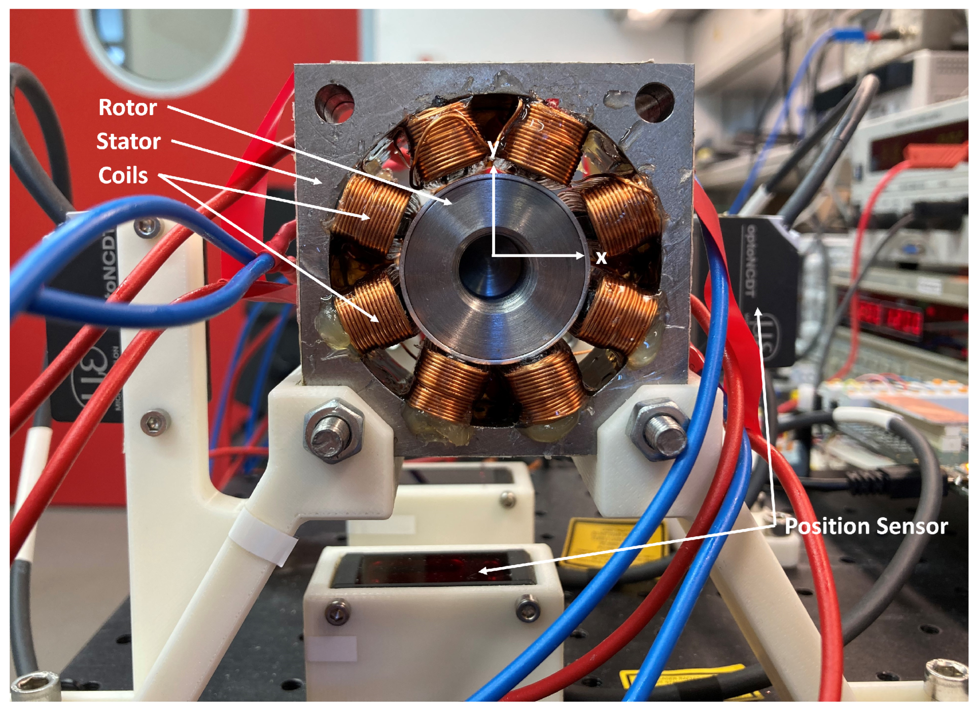Hence, reluctant-force-based AMBs require control algorithms with position feedback in order to stabilise the rotor at the centre position [1]. The position feedback is realised conventionally by additional sensors such as laser- or hall-effect sensors. However, sensors often are costly and require installation space and maintenance effort of the overall system, therefore weakening the economic merits of AMBs. In the past decades, sensorless control has been widely applied to AMBs to retrieve position information from electrical quantities already being measured in the system. Such a self-sensing approach can replace position sensors in cost-critical applications or provide further redundancy with existing position sensors in cases where high functional safety is required.

In the field of electrical machines, sensorless algorithms developed over the past decades are either based on the induced back-EMF or machine anisotropies. The review works [3,4,5] provide a good overview of existing techniques. In particular, there is a technique, which successfully exploits the star-point voltage and modified pulse width modulation (PWM). In some literature this technique is called Direct Flux Control [6,7,8,9,10,11].

These works demonstrate the robustness, accuracy and increased signal-to-noise ratio (SNR) of this approach. More in detail, there is another circuitry based on a re-settable integrator circuit that allows to amplify the star-point voltage with increased SNR. This approach seems interesting for future research works. Nevertheless, the technique requires not only an accessible star-point but also the modification of the PWM pattern, used to introduce zero voltage vectors and explicit, active voltage vectors for measurement. This puts several requirements on the switching power amplifier used. In a previous publication, such a power amplifier was introduced and validated [12]. The experimental validation of this driving approach showed satisfactory results. A detailed report can be found in [12].

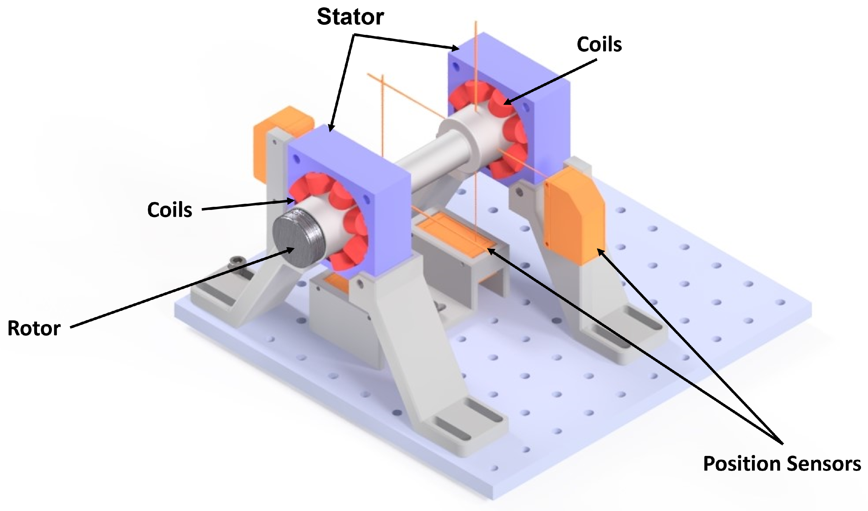
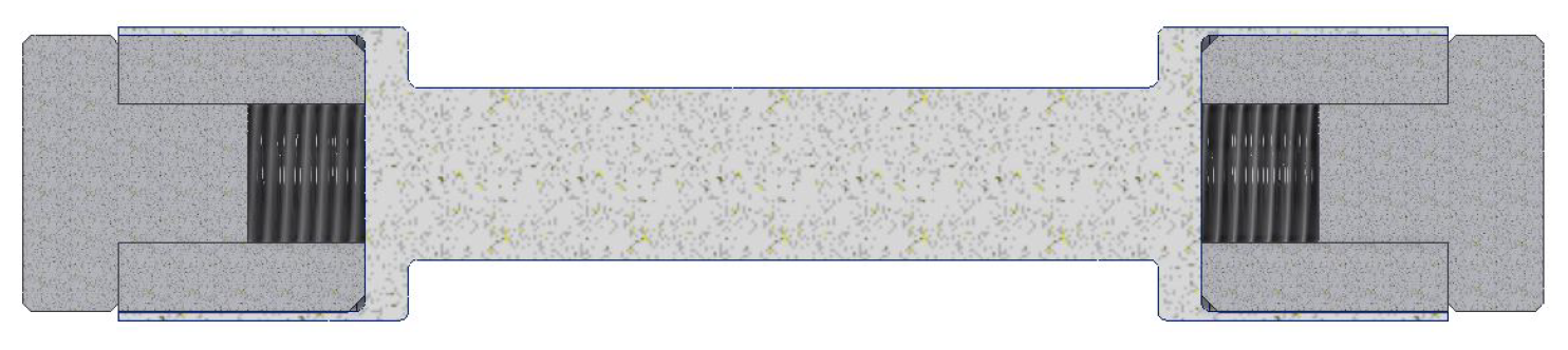
The aim of this work is to provide an elaborate position control strategy for the star-connected AMB. Since the test bench utilised in this application will also be used for teaching and demonstrating porpuses, a relatively large air gap has been chosen. This allows to observe the motion of the rotor with bare eyes and makes the technology easier accessible for students. In addition, the production of mechanical parts with higher tolerances is cost-effective and even enables the use of rapid prototyping. Thus, the control algorithm must be robust enough to compensate for the strong non-linearities of the AMB system. The most employed position controller in industrial applications is a Proportional Integral Derivative (PID) controller [1]. This type of controller is generally widely spread, well-documented and well-known by many engineers, making it easy to apply and tune. The PID controller delivers suitable and sufficient control performance for many fundamental applications. However, a review of active magnetic bearing control strategies finds that the PID controller cannot keep up with the demands of the most recent applications [13]. That is especially true for high-speed applications. This issue calls for novel control strategies for active magnetic bearings, which can stabilise the rotor at high speeds and reduce vibrations in the system. One way to achieve a better performance of the PID controller is the latter’s extension. The PID controller can be extended using fuzzy logic [14]. A comparison between PID and fuzzy-PID finds a better performance and lower energy consumption in the case of the fuzzy-PID controller [15]. Another way of improving the PID controller’s performance is using a neural network to update the controller’s gain during operation. A study finds good control performance and robustness to uncertainties compared to a plain PID controller [16]. A third method to extend the PID controller is fractional order control [17]. A study investigated the performance of a fractional order PID controller and found a distinct reduction of vibration compared to the plain PID controller [18]. A different control strategy is Flatness-Based control [19]. Experiments show a good performance considering trajectory tracking problems where the rotor is not held at a constant reference position but follows a given reference trajectory [20,21]. A further control strategy that gained attention is sliding mode control [22]. Experiments show a good disturbance rejection ability and good robustness to model uncertainties [23,24].

Comparing the different possibilities, the sliding mode control strategy seems most interesting for further research, because of its good robustness to model and parameter uncertainties, which is especially important with regard to the large air gap, since it induces strong non-linearities. Further, its lower computational and tuning effort, compared to strategies like fractional order PID control, makes it more easily applicable. Sliding mode control in all its varieties has been widely deployed to active magnetic bearings. Recent developments in sliding mode control focus on the theoretical and practical development of higher order sliding mode control algorithms, the discrete time implementation of sliding mode control and the application of sliding mode control to multi agent systems [25,26]. Similar to the PID controller, there are techniques that extend the sliding mode controller by adjusting its gains in order to ensure robustness and a finite time convergence on AMBs [26,27,28].

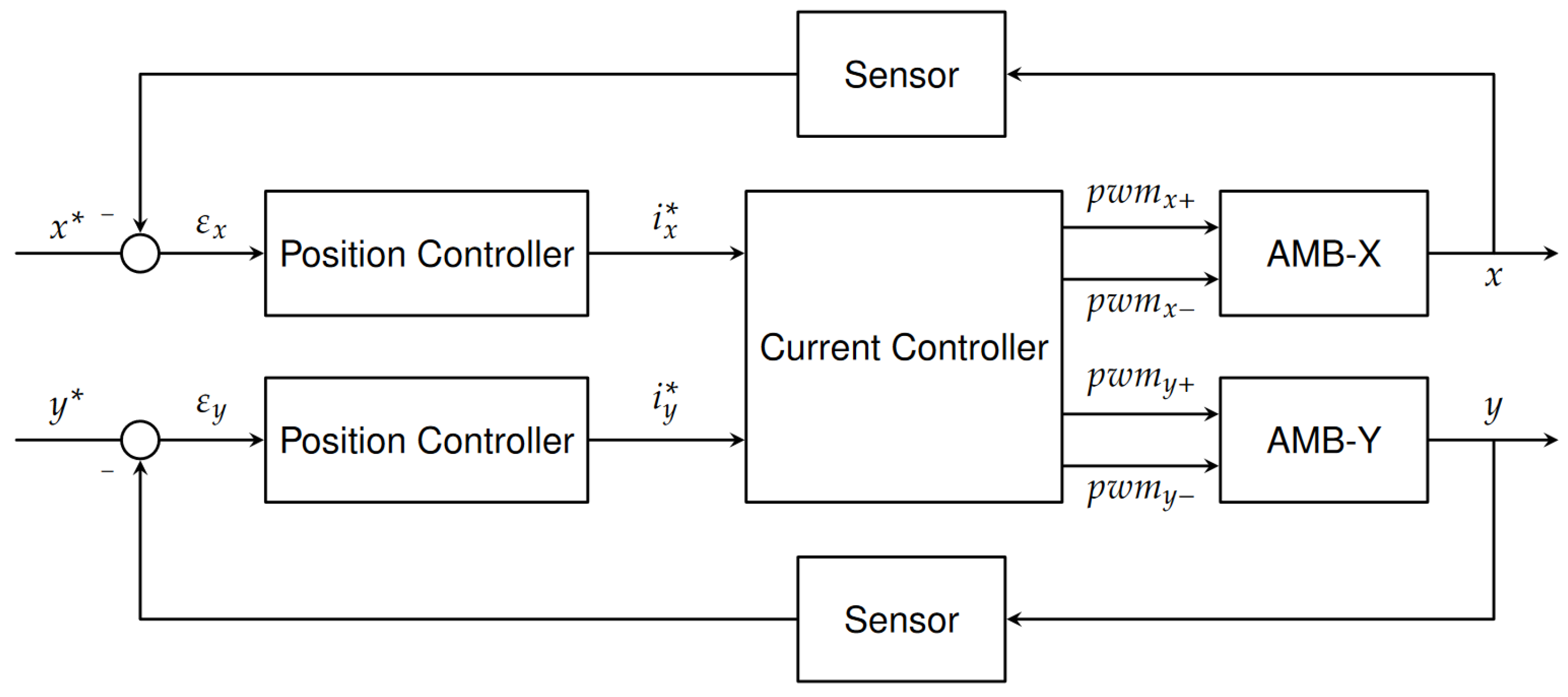
Many state of the art control strategies for AMBs rely on voltage control, where the cascading control loop, consisting of a position and a current controller, is integrated into one controller. This strategy is known to be beneficial for the overall performance of the AMB system [1]. On the other hand, integrating the current controller into the position controller makes it impossible to influence the current reference directly. However, the exertion of influence on the current reference can be beneficial for safety reasons, as the maximum current can easily be restricted. Further, the current controller can be tuned using a well-known industrial design criterion, which guarantees a specific and predefined current behaviour. An additional current limiting controller could also provide additional safety in the case of voltage control, but the current dynamics will still not feature a predefined behaviour.

To not leave behind the potential performance benefits, the aim is to integrate the dynamics of the current controller into the position controller model. This forms a cascading control loop consisting of a current controller with predefined behaviour, according to an industrial criterion and a position controller, that is aware of the current controller’s dynamics. A further potential benefit of the explicit current controller is the smoothing of the current reference from the sliding mode controller. Since sliding mode is known for its high-frequency switching nature, it seems beneficial to have a predefined bandwidth for the current dynamics. Especially since this control pattern will be used in further research regarding bandwidth-limited sensorless techniques.

Table A1. List of Symbols.

${\mathit{x}}^{\ast }$	reference displacement in x-direction
x	displacement in x-direction
$x_0$	initial rotor displacement in x-direction
$y^{\ast }$	reference displacement in y-direction
y	displacement in y-direction
$y_0$	initial rotor displacement in y-direction
$ϵ$	control error
u	controller output
i	current
$i_0$	bias current
f	force
${\mu }_0$	permeability of vacuum
${\mu }_r$	permeability of iron
n	number of windings in a coil
$A_a$	cross-section area
$\alpha$	angle between the legs of the AMB
$l_{fe}$	length of the iron
s	magnetic air gap
$s_0$	nominal magnetic air gap
$\mathsf{\Phi }$	magnetic flux
$W_a$	field energy
$V_a$	volume in the air gap
$B_a$	magnetic flux density in the air gap
$H_a$	magnetic field in the air gap
k	machine constant
$k_i$	force/current factor
$k_s$	force/displacement factor
v	velocity
m	mass of the rotor
L	inductance
R	resistance
$\tau$	time constant
$\mathit{x}$	state vector
$\sigma$	sliding variable
$\mathit{S}$	controller gain
c	controller gain
b	controller gain

and

Table A2. List of Indices.

*	control reference
x	in x direction
y	in x direction
+	in positive direction
−	in negative direction
R	state space description in controllability form

provide a list of the used symbols and indices.

2. Mathematical Modeling

2.1. Modelling of AMBs

The here-considered active magnetic bearings utilise reluctance forces. Reluctance forces are generated at the boundaries between materials with differing permeabilities $\mathsf{\mu }$. Figure 1 shows schematically the structure of a simple single-phase AMB and the magnetic flux $\mathsf{\Phi }$ along the iron with the length $l_{fe}$.

The calculation of reluctance forces is based on the field energy $W_a$. In a homogeneous field, the energy stored in an air gap with size s, a cross-sectional area A and a volume $V_a=2s{A}_a$ can be written as [1,29]:

$$\begin{array}{c}\hfill W_a=\frac{1}{2}{B}_a{H}_a{V}_a=\frac{1}{2}{B}_a{V}_a{A}_{a}2s=B_a{V}_a{A}_{a}s.\end{array}$$

(1)

Here, $B_a$ denotes the magnetic flux density in the air gap and $H_a$ denotes the magnetic field in the air gap, respectively. The force f equals the partial derivative of $W_a$ with respect to the air gap (displacement) s [1,29,30]:

$$\begin{array}{c}\hfill f=-\frac{\partial W_a}{\partial s}=B_a{H}_a{A}_a.\end{array}$$

(2)

Inserting the constitutive law $B={\mu }_0{\mu }_{r}H$ yields:

$$\begin{array}{c}\hfill f=\frac{{B_a}^2{A}_a}{{\mu }_0}.\end{array}$$

(3)

According to [1,29,30], the magnetic circuit in Figure 1 can be described using the number of the coil windings n and the current i flowing through the coils:

$$\begin{array}{c}\hfill B={\mu }_0\frac{ni}{2s}.\end{array}$$

(4)

Assuming the flux density remains constant along the iron with length $l_{fe}$ and the air gap s, the force of an AMB can be obtained by inserting Equation (4) into Equation (3):

$$\begin{array}{c}\hfill f={\mu }_0{A}_a{\left(\frac{ni}{2s}\right)}^2=\frac{1}{4}{\mu }_0{n}^2{A}_a\frac{i^2}{s^2}.\end{array}$$

(5)

A new variable k is introduced to simplify the equation:

$$\begin{array}{c}\hfill f=k\frac{i^2}{s^2},\end{array}$$

(6)

with

$$\begin{array}{c}\hfill k=\frac{1}{4}{\mu }_0{n}^2{A}_a.\end{array}$$

(7)

As the poles of the electromagnet affect the rotor with an angle $\alpha$, the force f of the AMB in Figure 1 can be obtained by [1,29]:

$$\begin{array}{c}\hfill f=k\frac{i^2}{s^2}cos\alpha .\end{array}$$

(8)

Equation (8) indicates, that the force depends quadratically on the current and inverse quadratically on the air gap. Since the force depends quadratically on the current, the force is independent of the sign of the current and always acts in the same direction, namely towards the electro magnet. However, in control theory, linear relations are preferred. Often, non-linear relationships are approximated in the operating point. For an active magnetic bearing, the operating point is defined by a bias current $i_0$ and the nominal air gap $s_0$.

Further, there are often two electromagnets opposite to each other, as shown in Figure 2. In order to generate counteracting forces, the upper magnet is driven with the sum of the bias current $i_0$ and the control current $i_x$. Instead, the lower magnet is driven by the difference between the bias current $i_0$ and the control current $i_x$. This configuration is called differential driving mode [1,29,30].

The force $f_x$ can now be represented as the difference between the forces of the two magnets $f_{+}$ and $f_{-}$, respectively [1,29]:

$$\begin{array}{c}\hfill f_x=f_{+}-f_{-}=k\left(\frac{{(i_0+i_x)}^2}{{(s_0-x)}^2}-\frac{{(i_0-i_x)}^2}{{(s_0+x)}^2}\right)cos\alpha .\end{array}$$

(9)

Equation (9) can be simplified and linearised with respect to $x\ll s_0$ [1]:

$$\begin{array}{cc}\hfill f_x& \hfill =\frac{4k{i}_0}{s_0^2}\left(cos\alpha \right)i_x+\frac{4k{i}_0^2}{s_0^3}\left(cos\alpha \right)x,\hfill \end{array}$$

(10)

$$\begin{array}{cc}\hfill f_x& \hfill =k_i{i}_x-k_{s}x,\hfill \end{array}$$

(11)

with

$$\begin{array}{c}\hfill k_i=\frac{4k{i}_0}{s_0^2}cos\alpha ,\end{array}$$

(12)

and

$$\begin{array}{c}\hfill k_s=-\frac{4k{i}_0^2}{s_0^3}cos\alpha .\end{array}$$

(13)

Equations (12) and (13) show that the force/current and the force/displacement factors depend quadratically and cubic, respectively, on the air gap. As mentioned, a linear relationship is preferred for the control. Hence, both factors are linearised in the operating point as illustrated in Figure 3. Due to this linearisation, large parameter deviations can be expected when leaving the operating point.

While deriving this model, approximations have been made to simplify the physical correlations. The surface of the ferromagnetic material $A_{fe}$ and the projected surface of the air gap $A_a$ will not be equal in an actual application. Further, flux leakage along the air gap must be expected. Moreover, material properties, such as hysteresis, saturation and losses in copper and iron, such as eddy current and hysteresis losses, have been neglected. Mechanical losses due to friction between the rotor and the medium surrounding it have not been modelled. The considered rotor is rigid, symmetric and gyroscopic effects are neglected. With these approximations, the error calculating the force lies within the range from 5 to 10% [1].

However, in order to design a sliding mode controller, the description must be available in the state space and ideally, in the controllability form [31]. The controllability form allows to easily read the relationship between the eigenvalues of the system and the model parameters. Further, the existence of the controllability form shows that the system is indeed controllable. The previously derived differential equations can be transformed into a state space description by introducing the displacement x of the rotor and its velocity $v=\dot{x}$ as the two states of the system:

$$\begin{array}{c}\hfill \mathit{x}=\left[\begin{array}{c}x\\ v\end{array}\right].\end{array}$$

(14)

For a system in the state space:

$$\begin{array}{c}\hfill \dot{x}\left(t\right)=\mathit{A}\mathit{x}\left(t\right)+\mathit{b}u\left(t\right),\end{array}$$

(15)

$$\begin{array}{c}\hfill y\left(t\right)=\mathit{c}\mathit{x}\left(t\right)+du\left(t\right),\end{array}$$

(16)

this yields the following system in matrix notation:

$$\begin{array}{cc}\hfill \mathit{A}& \hfill =\left[\begin{array}{cc}0& 1\\ -\frac{ks}{m}& 0\end{array}\right],\mathit{b}=\left[\begin{array}{c}0\\ \frac{k_i}{m}\end{array}\right],\hfill \end{array}$$

(17)

$$\begin{array}{cc}\hfill {\mathit{c}}^{⊺}& \hfill =\left[\begin{array}{cc}1& 0\end{array}\right],\hfill \end{array}$$

(18)

$$\begin{array}{cc}\hfill d& \hfill =0,\hfill \end{array}$$

(19)

$$\begin{array}{cc}\hfill \mathit{x}\left(0\right)& \hfill ={\mathit{x}}_0.\hfill \end{array}$$

(20)

This system is not yet in the desired controllability form, but can be transferred into the following system [31,32]:

$$\begin{array}{cc}\hfill {\mathit{A}}_R& \hfill =\left[\begin{array}{cc}0& 1\\ -\frac{ks}{m}& 0\end{array}\right],{\mathit{b}}_R=\left[\begin{array}{c}0\\ 1\end{array}\right],\hfill \end{array}$$

(21)

$$\begin{array}{cc}\hfill {\mathit{c}}_R^{⊺}& \hfill =\left[\begin{array}{cc}\frac{k_i}{m}& 0\end{array}\right],\hfill \end{array}$$

(22)

$$\begin{array}{cc}\hfill d& \hfill =0,\hfill \end{array}$$

(23)

$$\begin{array}{cc}\hfill {\mathit{x}}_R\left(0\right)& \hfill ={\mathit{x}}_{R0},\hfill \end{array}$$

(24)

which represents the controllability form.

2.2. Integrating the Current Controller Dynamics

Figure 4 shows the current control loop and its components. The PI controller, voltage amplifier and coils are in the forward path and the current sensor is in the backwards path, all with their corresponding transfer functions:

• PI Controller: $K_{pi}\frac{1+{\tau }_{ii}s}{{\tau }_{ii}s}$ with the controller gain $K_{pi}$ and the time constant ${\tau }_{ii}$ tuned according to the modulus optimum criterion.
• H-bridge Voltage Amplifier: $\frac{1}{1+{\tau }_{A}s}$ with the time constant ${\tau }_A=\frac{1}{2f_A}$ where $f_A$ is the PWM frequency of the H-bride.
• Current Sensor: $\frac{1}{1+{\tau }_{s}s}$ with its time constant ${\tau }_s=\frac{1}{f_s}$, where $f_s$ is the sensors sampling frequency.
• Coil: $\frac{1}{R(1+{\tau }_{a}s)}$ with is resistance R, inductance L, gain $\frac{1}{R}$ and its electric time constant ${\tau }_a=\frac{L}{R}$.

As mentioned, the PI current controller is tuned according to the industrial modulus optimum criterion, in order to achieve a predefined behaviour [12,33]. The PI controller’s time constant ${\tau }_{ii}$ can be set as ${\tau }_{ii}={\tau }_a$, which then cancels the slowest time constant. The PI controllers gain $K_{pi}$ is tuned according to the modulus optimum criterion:

$$\begin{array}{c}\hfill K_{pi}=\frac{R_a{\tau }_a}{2{\tau }_{\mathsf{\Sigma }}}.\end{array}$$

(25)

The current control loop can be simplified with respect to the modulus optimum criterion, so the feedback loop can be expressed as [33]

$$\begin{array}{c}\hfill G_{PI}\left(s\right)=\frac{1}{2{\tau }_{\mathsf{\Sigma }}^2{s}^2+2{\tau }_{\mathsf{\Sigma }}s+1}.\end{array}$$

(26)

Here, ${\tau }_{\mathsf{\Sigma }}$ is the sum of the time constants of the current sensor ${\tau }_s$ and the time constant of the voltage amplifier ${\tau }_A$. This transfer function now features a maximum overshoot of 4%, a rise time of 4.5${\tau }_{\mathsf{\Sigma }}$, a settling time of 8.4${\tau }_{\mathsf{\Sigma }}$ and a control error of $\pm 2\%$ [33].

The transformation of Equation (26) yields the following state space description [31,32]:

$$\begin{array}{cc}\hfill {\mathit{A}}_{pi}& =\left[\begin{array}{cc}0& 1\\ -\frac{1}{2{\tau }_{\mathsf{\Sigma }}^2}& -\frac{1}{{\tau }_{\mathsf{\Sigma }}}\end{array}\right],{\mathit{b}}_{pi}=\left[\begin{array}{c}0\\ 1\end{array}\right],\hfill \\ \hfill {\mathit{c}}_{pi}^{⊺}& =\left[\begin{array}{cc}\frac{1}{2{\tau }_{\mathsf{\Sigma }}^2}& 0\end{array}\right],\hfill \\ \hfill d& =0.\hfill \end{array}$$

(27)

The states are choosen as:

$$\begin{array}{c}\hfill \mathit{x}=\left[\begin{array}{c}i\\ \frac{di}{dt}\end{array}\right].\end{array}$$

(28)

Now, both cascading subsystems have been derived and need to be integrated. This yields the following controllable system in the state space:

$$\begin{array}{cc}\hfill \mathit{A}& =\left[\begin{array}{cccc}0& 1& 0& 0\\ 0& 0& 1& 0\\ 0& 0& 0& 1\\ -\frac{k_s}{2m{\tau }_{\mathsf{\Sigma }}^2}& -\frac{k_s}{m{\tau }_{\mathsf{\Sigma }}}& \frac{2k_s{\tau }_{\mathsf{\Sigma }}^2+m}{2m{\tau }_{\mathsf{\Sigma }}^2}& -\frac{1}{{\tau }_{\mathsf{\Sigma }}}\end{array}\right],\mathit{b}=\left[\begin{array}{c}0\\ 0\\ 0\\ 1\end{array}\right],\hfill \\ \hfill {\mathit{c}}^{⊺}& =\left[\begin{array}{cccc}\frac{k_i}{2m{\tau }_{\mathsf{\Sigma }}}& 0& 0& 0\end{array}\right],\hfill \\ \hfill d& =0.\hfill \end{array}$$

(29)

With the state vector:

$$\begin{array}{c}\hfill \mathit{x}={\mathit{T}}_{\mathit{R}}^{-1}\left[\begin{array}{c}i\\ \frac{di}{dt}\\ x\\ v\end{array}\right],{\mathit{x}}_{\mathit{R}\mathit{0}}={\mathit{T}}_{\mathit{R}}^{-1}{\mathit{x}}_{\mathit{0}}=0,\end{array}$$

(30)

and

$$\begin{array}{c}\hfill {\mathit{T}}_{\mathit{R}}=\left[\begin{array}{cccc}\frac{k_s}{m}& 0& 1& 0\\ 0& \frac{k_s}{m}& 0& 1\\ \frac{k_i}{2m{\tau }_{\mathsf{\Sigma }}^2}& 0& 0& 0\\ 0& \frac{k_i}{2m{\tau }_{\mathsf{\Sigma }}^2}& 0& 0\end{array}\right].\end{array}$$

(31)

Here, $T_R$ denotes the transformation matrix into the controllability from.

3. Controller Design

The goal is now, to design a controller that drives the rotor to the referenced position and stabilises it. As mentioned in the previous section, the AMB model is fraught with uncertainties. Further, the AMB has a highly nonlinear behaviour that has been linearised in the operating point. However, since the operating point is left in phases such as the startup, large parameter deviations must be taken into account. For these reasons, sliding mode control has been chosen for its robustness against model and parameter uncertainties.

After the desired dynamics were derived previously, the sliding variable can be introduced:

$$\begin{array}{c}\hfill \sigma =\sigma \left(\mathit{x}\right).\end{array}$$

(32)

Sliding mode control aims to drive $\sigma$ to zero in finite time by employing a control law $u=u\left(x\right)$. In the case of the AMB, the controller output is equivalent to the current reference $u=u\left(x\right)=i^{\ast }$. Thus, sliding mode control can be considered a two-part controller design, consisting of a switching function $\sigma \left(x\right)$ and a control law $u\left(x\right)$.

For a system described in the state space

$$\begin{array}{c}\hfill \dot{\mathit{x}}\left(t\right)=\mathit{Ax}\left(t\right)+\mathit{b}u\left(t\right),\end{array}$$

(33)

a switching function can be defined as

$$\begin{array}{c}\hfill \sigma \left(\mathit{x}\right)=\mathit{S}\mathit{x}\left(t\right),\end{array}$$

(34)

with

$$\begin{array}{c}\hfill \mathit{S}\in {\mathbb{R}}^n.\end{array}$$

(35)

$\mathit{S}$ is a free parameter. Literature states that it is not entirely transparent, how to select a value for $\mathit{S}$ in order to ensure a specific design criterion [34]. However, there are well-studied systematic and traceable methods that provide a range of values for the design of $\mathit{S}$, one of which is the pole-placement method [34,35]. If a system is given in the previously mentioned controllability form, a suitable switching function is given by [34]:

$$\begin{array}{c}\hfill \sigma \left(\mathit{x}\right)=s_1{x}_1+s_2{x}_2+...+s_{n-1}{x}_{n-1}+x_n.\end{array}$$

(36)

However, to counteract the widely differing magnitudes of the states, the switching function for the AMB is now chosen in a more general form as

$$\begin{array}{c}\hfill \sigma \left(\mathit{x}\right)=s_{1}i+s_2\frac{di}{dt}+s_{3}x+s_{4}v.\end{array}$$

(37)

This switching function results in a high-frequency switching motion in the control action, causing the so-called chattering phenomenon. On the other hand, the switching function is also the root of the robustness against parameter and model uncertainties. Having the current and its derivative integrated into the switching function, allows the sliding mode controller to counteract the otherwise unknown disturbances induced by the current control loop.

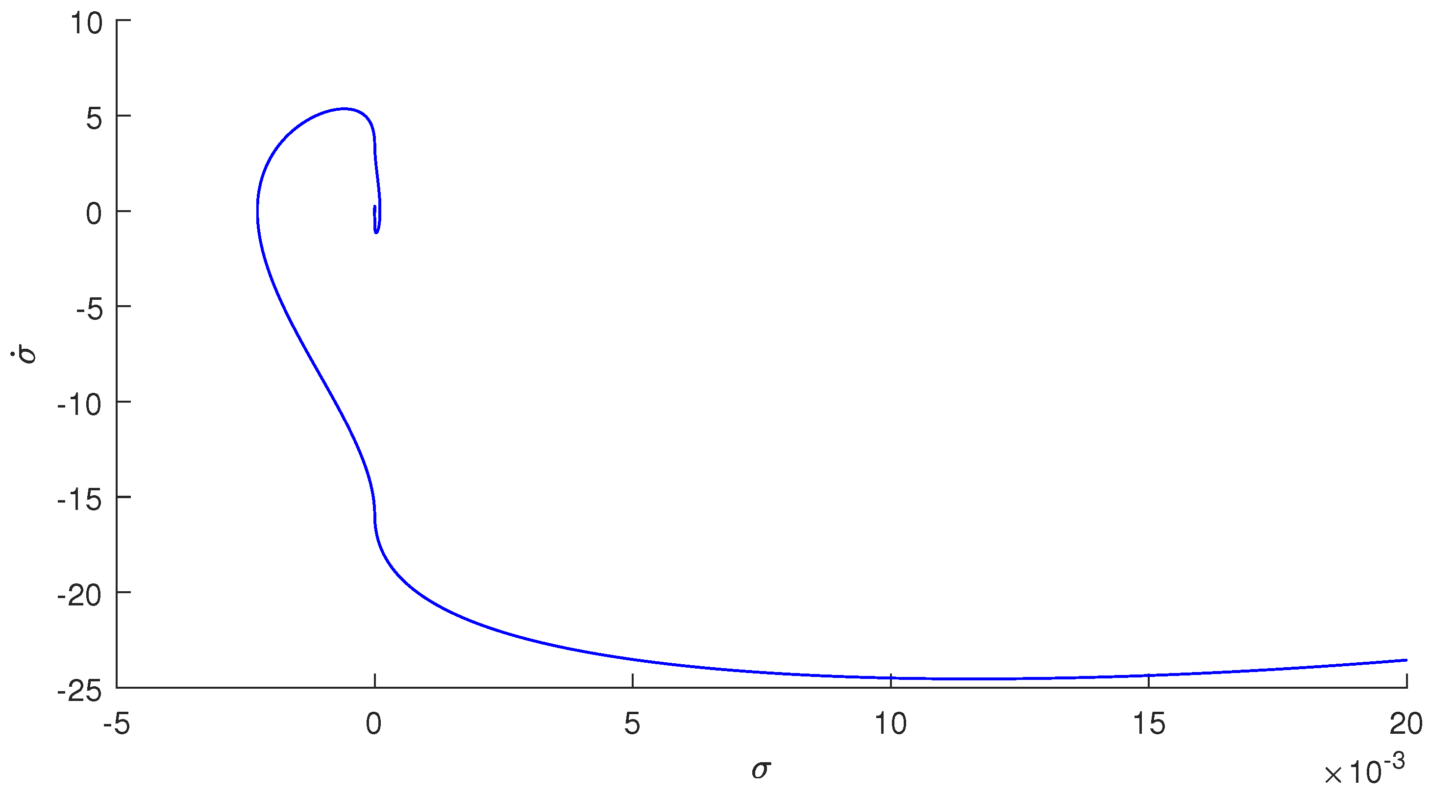
For the part of the control law, the conventional sliding mode is especially known for the chattering phenomenon. Chattering can be a severe issue in cascade control systems, such as a magnetic bearing with an explicit current controller [35]. For this reason, the conventional sliding mode is considered unsuitable and second-order sliding mode is employed. Figure 5 shows that, in contrast to the conventional sliding mode, second order sliding mode drives not only $\sigma$ to zero but also its derivative $\dot{\sigma }$. In theory, second-order sliding mode is free of chattering. In reality, however, discretisation and disturbances add residual chattering. Several algorithms induce a second-order sliding motion in the system. Since $\dot{\sigma }$ needs to be driven to zero as well, additional measurements are often necessary. In reality, however, this is often not feasible because additional sensors would be needed. This narrows down the choice for a second-order sliding mode control algorithm. The only algorithm that does not require a measurement of $\dot{\sigma }$ is the so-called super-twisting control algorithm. The algorithm is given by [34,35]:

$$\begin{array}{c}\hfill \begin{array}{cc}\hfill u& =c\sqrt{\left|\sigma \right|}sign\left(\sigma \right)+w,c=1.5\sqrt{C};b=1.1C,\hfill \\ \hfill \dot{w}& =bsign\left(\sigma \right).\hfill \end{array}\end{array}$$

(38)

The parameters c and b are positive scalar controller gains. The scalar C symbolises the Lipschitz constant for unknown but bounded disturbances. Other than the conventional sliding mode, super twisting control is a continuous control algorithm. The high-frequency switching function is now hidden under the integral

$$\begin{array}{c}\hfill w=b\int sign\left(\sigma \right)dt.\end{array}$$

(39)

The proposed controller design introduces the dynamics of the current control loop into the sliding mode controller without having to abandon the explicit current controller. This way, the proposed design tries to combine the advantages of the a current controlled schema, like easy exertion of influence on the current, with the performance boost of a voltage control schema.

4. Results and Discussion

4.1. Test Bench Design

In order to validate the derived control approach, a test bench consisting of two individual two-degree of freedom (DOF) bearings is engineered. Both bearings work independently of each other and shift in axial direction is neglected in this prototype application. Thus, no additional thrust bearing is provided and the rotor is only supported in x- and y-direction. However, due to the reluctant forces, the rotor is still supported passively in z-direction. Figure 6 shows the control loop for one single bearing. The control loop consists of two independent position controllers for x- and y-axis. The current references $i_x^{\ast }$ and $i_y^{\ast }$ respectively, are fed into the current controller. The current controller supplies the demanded current across the star connected coils of the AMB utilizing a PWM pattern. The bearing consists of 4 coil pairs in differential driving mode, two per axis, as displayed in Figure 2. The current control loop, as described earlier, and the corresponding hardware are explained in detail in the previous publication [12].

Figure 7 shows a 3D model of the test bench. Each bearing consists of an 8-pole stator with a heteropolar coil arrangement (blue). The 8 coils (red) have 96 windings each and are interconnected to pairs. The position of the rotor is measured by a total of four position sensors (orange), that operate at a sampling frequency of 2 kHz. The rotor is composed of an aluminium hull (light grey) and 2 ferromagnetic cores (darker grey), which are embedded in the hull at each end. This construction prevents magnetic “sticking” in the event of a touchdown or in the startup phase. Figure 8 and Figure 9 illustrate this design with a 3D Model of the used rotor and a cross-section. This design leads to a nominal mechanical air gap of 1 mm and a nominal magnetic air gap of 2 mm, meaning the outer aluminium hull has a thickness of 1mm. Figure 10 shows the front view on the bearing, with clearly visible coils, stator and rotor.

The current reference from the derived sliding mode controller is fed into the modulus optimum tuned PI current controller. Utilizing PWM, the current controller supplies the requested current across the star-connected coils. The current controller and the star connection are investigated and explained in [12]. Parameters of the test bench and controller gains can be found in Appendix B.

The build test bench and the model from Section 2 were validated against each other with respect to the force current relation ship. The force current relationship from Equation (11) can be easily validated by comparing the actual current necessary to levitate the rotors weight to the theoretical current according to Equation (11). For a rotor weighting 406 g and an average current of 0.77 A this yields an error of $5.97\%$ for the force current factor. This is within the 5–10% error expectation due to the unmodelled losses in the system, explained in Section 2 [1].

4.2. Experiment Current Controlled

In the first experiment, only one bearing is active and the current controlled system from Equations (22)–(24) is considered. Thus, there is no compensation for the current controller dynamics. The second bearing is turned off and remains idle. The experiment starts from the rest position, where the rotor is in contact with the lower part of the stator, and a constant reference displacement $x_{ref}=0$. Figure 11 shows the error in the displacement and the current reference during the experiment. During this experiment, the rotor can lift off without any external help. After the rotor position is stable, an increasing manual force in the negative y-direction (downwards) followed by force in the positive y-direction (upwards) is applied from seconds two to six and seven to ten. The current reference returns to the unloaded level and sinks according to the force. During the changes in the load, the controller manages to keep the rotor in a stable position. At second 11.5, the rotor contacts the lower stator, enforced by a large external force. At second 14.5, the external force is applied in the opposite direction, forcing the rotor to contact the upper stator. Just as at the beginning of the experiment, the rotor can recover from rest-position and forced touch-down without external help or a specific startup or touchdown sequence. The controller remains stable, despite the relatively large air gap and the associated leaving of the operating point. This recovery underlines the robust controller design. The rotor moves within ±0.15 mm range, except for the forced touchdowns.

Table 1. Error metrics of the experiment neglecting current controller dynamics, with one bearing, constant reference positions and external disturbance forces.

Axis	Mean Error in %	Max Error in %	Max Error in mm	Settling Time in s
x	0.9	21.18	0.21	0.7
y	0.44	15.42	0.15	0.7

shows the error metric for this experiment. The defined error metrics are the mean error in % of the nominal mechanical air gap (1 mm) after initial rotor lift-off, the absolute maximum error in % of the nominal mechanical air gap (1 mm) after the initial rotor lift-off, the maximal error in mm, and the approximate settling time of the rotor at the beginning of the experiment in seconds. All metrics are provided for the x- and y-axis and measured without external disturbance forces. The maximum error in x direction is higher compared to the error in y direction because mechanical vibrations are influencing the measurement in this particular case.

The next experiment considers the system from Equation (30). The additional states, current and current derivative, were added to the sliding surface to improve the position controllers performance. This experiment is conducted with only one bearing operating. Again, the error in the displacement and the current reference are displayed in Figure 12. The rotor can lift off without external help and starts vibrating in the range of $\pm 20$$\mathsf{\mu }$m after stabilising. This is already a notable improvement compared to the controller without current controller dynamics.

Table 2. Error metrics of the experiment with current controller dynamics and constant reference positions.

Axis	Mean Error in %	Max Error in %	Max Error in mm	Settling Time in s
x	0.007	1.86	0.018	0.6
y	0.03	1.86	0.018	0.6

provides the error metrics for this experiment.

On the other hand, chattering in the current reference increased considerably. The dynamic of the current is much faster than the one of the position. Thus the sliding motion attained a high-frequency component. The chattering frequency rose from 40 Hz to 300 Hz, and the amplitude gained approximately ±0.2 A.

The experiment is conducted again, now with both bearings operating. The displacement error oscillates around the reference position in the range of $\pm 0.1$ mm as Figure 13 shows. Again the addition of the high-frequency dynamic of the current results in more chattering in the current reference. It is clearly visible, that the unmodelled rotor dynamics add further disturbances. However, the rotor remains stable around the reference position in the presence of the mentioned, unmodelled dynamics, which speaks in favour of a robust controller. The rotor can still lift off from the initial rest position without external help.

Table 3. Error metrics of experiment with current controller dynamics and both bearings operating.

Axis	Mean Error in %	Max Error in %	Max Error in mm	Settling Time in s
x	0.14	12.32	0.12	0.6
y	0.11	14.48	0.14	0.6

provides the error metrics for this experiment as defined earlier.

5. Conclusions

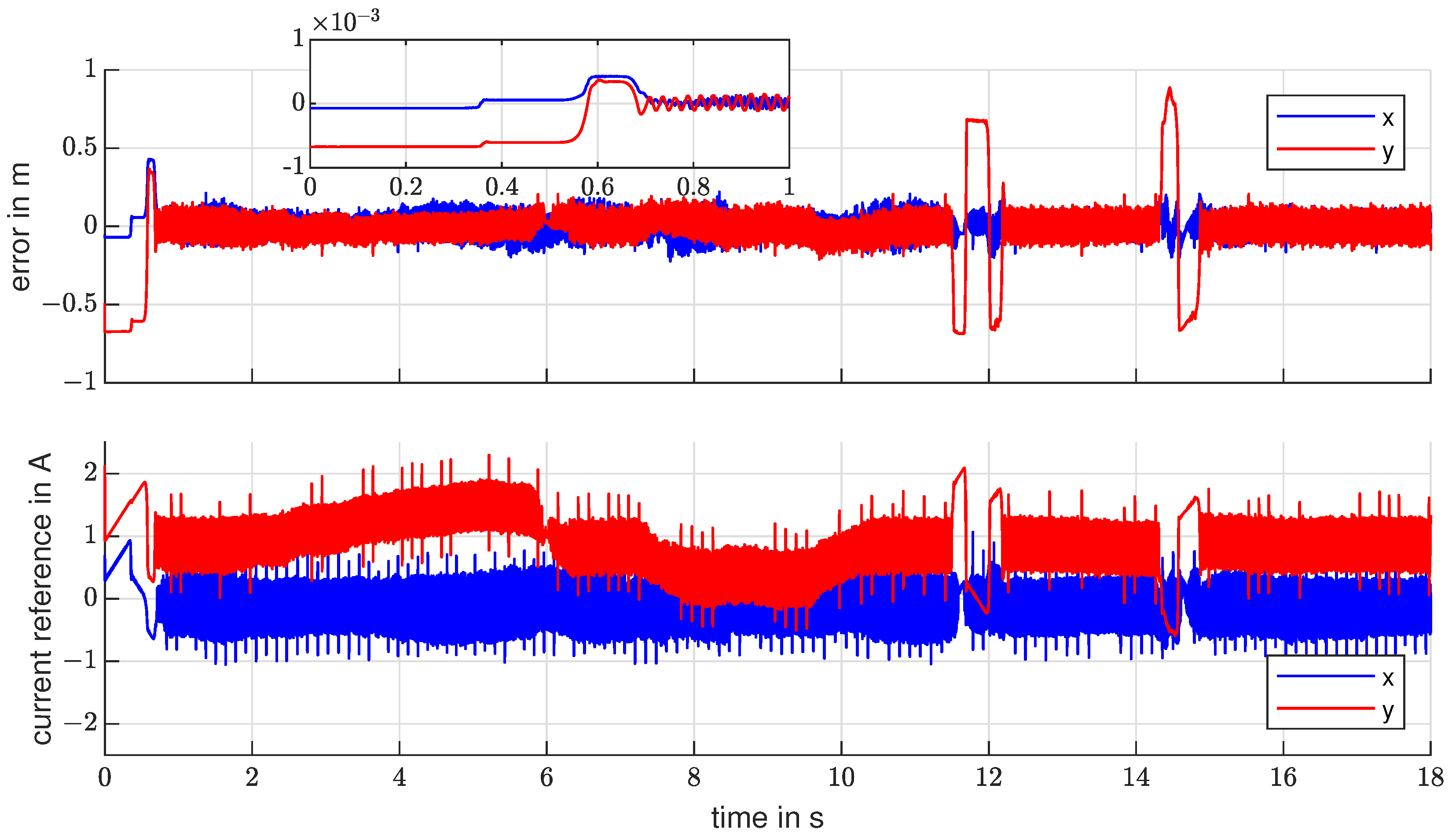
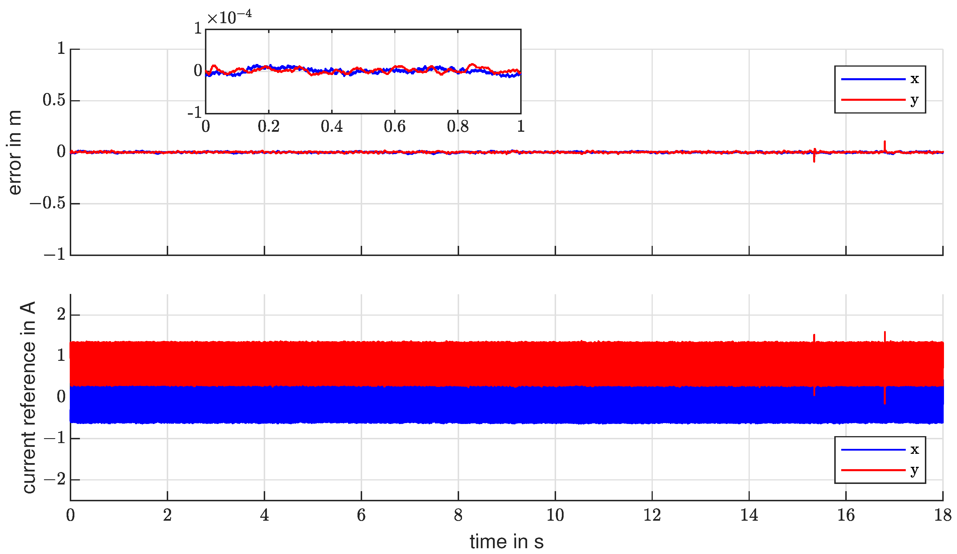
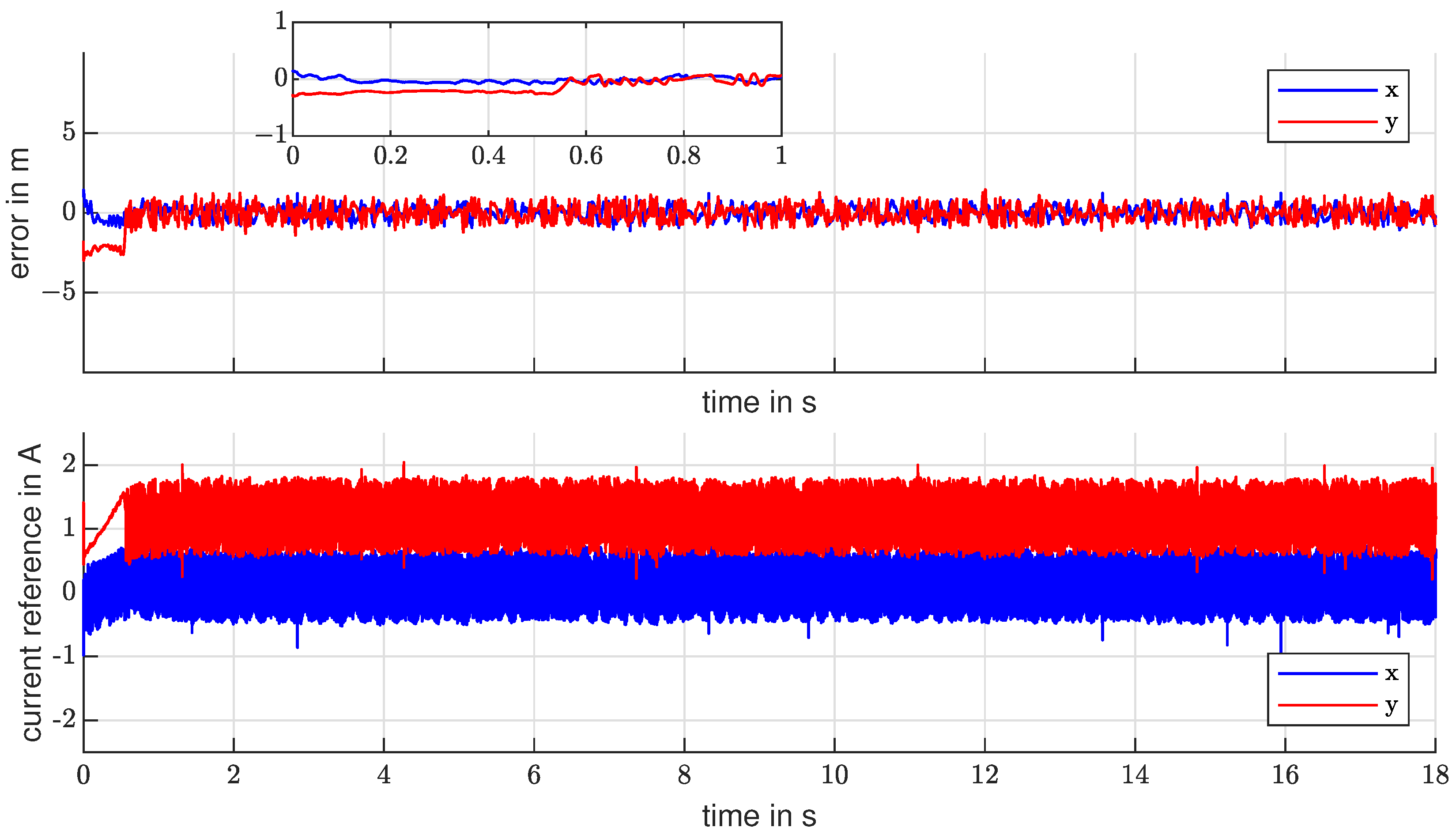
This work proposes a position control strategy for a four-phase star-connected AMB, that integrates the dynamics of the nested, explicit current controller into the position controller. In the experiments, the controller is able to lift from an initial rest position and to levitate the rotor around the reference position which proves to be robust against external disturbance forces. Further, the controller is robust enough to withstand the strong non-linearities and the left of the operating point during the touchdown and startup phases. This is particularly noteworthy because of the large air gap, which introduces large model parameter variations. Integrating the current controller dynamics improves the controller accuracy by about 87% letting the rotor oscillate around the reference position within the range of $\pm 20$$\mathsf{\mu }$m or 1% of the magnetic air gap size, considering only one bearing is operating. At the same time, the other is in rest position. On the other hand, the chattering frequency increased distinctly, rising up by 650% to 300 Hz. The amplitude of the chattering motion in the control reference $i^{\ast }$ also gained approximately 40%. Considering both bearings operating, the rotor oscillates within $\pm 1$ mm or 5% of the total air gap. The controller is able to recover from touchdown and rest position without external help. A study carried out with a similar model and similar model parameters for sliding mode control for AMBs gave consistent results for the system without current controller dynamics [23]. Compared to this study the integration of the current controller dynamics reduces the trajectory range of the rotor in a stable position by about 83%.

The proposed controller provides increased performance for active magnetic bearing systems with star-connected coils and therefore allows the exploitation of the star point voltage for sensorless position estimation for AMBs. Latter will be the focus of further research. Further, the advancement of the position control strategy, for example by considering the now unmodelled dynamics of the rotor, will be studied.

References

1. Maslen, E.H.; Schweitzer, G. (Eds.) Magnetic Bearings; Springer: Berlin/Heidelberg, Germany, 2009. [Google Scholar] [CrossRef]
2. Earnshaw, S. On the nature of the molecular forces which regulate the constitution of the luminferous ether. Trans. Camb. Philos. Soc. 1842, 7, 97. [Google Scholar]
3. Benjak, O.; Gerling, D. Review of position estimation methods for IPMSM drives without a position sensor part II: Adaptive methods. In Proceedings of the XIX International Conference on Electrical Machines—ICEM 2010, Rome, Italy, 6–8 September 2010; IEEE: Piscataway, NJ, USA, 2010. [Google Scholar] [CrossRef]
4. Benjak, O.; Gerling, D. Review of Position Estimation Methods for PMSM Drives Without a Position Sensor, Part III: Methods based on Saliency and Signal Injection. In Proceedings of the 2010 International Conference on Electrical Machines and Systems, Incheon, Republic of Korea, 10–13 October 2010. [Google Scholar]
5. Benjak, O.; Gerling, D. Review of position estimation methods for IPMSM drives without a position sensor part I: Nonadaptive methods. In Proceedings of the The XIX International Conference on Electrical Machines—ICEM 2010, Rome, Italy, 6–8 September 2010; IEEE: Piscataway, NJ, USA, 2010. [Google Scholar] [CrossRef]
6. Strothmann, R. Fremderregte Elektrische Maschine. EP Patent EP1005716B1, 14 November 2001. [Google Scholar]
7. Mantala, C. Sensorless Control of Brushless Permanent Magnet Motors. Ph.D. Thesis, University of Bolton, Bolton, UK, 2013. [Google Scholar]
8. Schuhmacher, K.; Grasso, E.; Nienhaus, M. Improved rotor position determination for a sensorless star-connected PMSM drive using Direct Flux Control. J. Eng. 2019, 2019, 3749–3753. [Google Scholar] [CrossRef]
9. Werner, T. Geberlose Rotorlagebestimmung in Elektrischen Maschinen; Springer Fachmedien Wiesbaden: Wiesbaden, Germany, 2018. [Google Scholar] [CrossRef]
10. Grasso, E.; Mandriota, R.; König, N.; Nienhaus, M. Analysis and Exploitation of the Star-Point Voltage of Synchronous Machines for Sensorless Operation. Energies 2019, 12, 4729. [Google Scholar] [CrossRef]
11. Grasso, E. Direct Flux Control—A Sensorless Technique for Star-Connected Synchronous Machines An Analytic Approach; Shaker Verlag: Düren, Germany, 2021. [Google Scholar]
12. Brasse, R.; Vennemann, J.; König, N.; Grasso, E.; Nienhaus, M. Design and Implementation of a Driving Strategy for Star-Connected Active Magnetic Bearings with Application to Sensorless Driving. Engergies 2023, 16, 396. [Google Scholar] [CrossRef]
13. Huang, T.; Zheng, M.; Zhang, G. A Review of Active Magnetic Bearing Control Technology. In Proceedings of the 2019 Chinese Control And Decision Conference (CCDC), Nanchang, China, 3–5 June 2019; IEEE: Piscataway, NJ, USA, 2019; pp. 2888–2893. [Google Scholar] [CrossRef]
14. Zadeh, L. Fuzzy logic. Computer 1988, 21, 83–93. [Google Scholar] [CrossRef]
15. Psonis, T.; Mitronikas, E.; Nikolakopoulos, P. Comparison of PID and Fuzzy PID Controller for a Linearised Magnetic Bearing. Tribol. Ind. 2017, 39, 349–356. [Google Scholar] [CrossRef] [Green Version]
16. Chen, S.Y.; Lin, F.J. Decentralized PID neural network control for five degree-of-freedom active magneticbearing. Eng. Appl. Artif. Intell. 2013, 26, 962–973. [Google Scholar] [CrossRef]
17. Shah, P.; Agashe, S. Review of fractional PID controller. Mechatronics 2016, 38, 29–41. [Google Scholar] [CrossRef]
18. Shata, A.M.A.H.; Hamdy, R.A.; Abdelkhalik, A.S.; El-Arabawy, I. A fractional order PID control strategy in active magnetic bearing systems. Alex. Eng. J. 2018, 57, 3985–3993. [Google Scholar] [CrossRef]
19. Rudolph, J. Flatness-Based Control An Introduction; Shaker Verlag: Düren, Germany, 2021. [Google Scholar]
20. Lévine, J.; Lottin, J.; Ponsart, J.C. Control of Magnetic Bearings: Flatness with Constraints. IFAC Proc. Vol. 1996, 29, 2798–2803. [Google Scholar] [CrossRef]
21. von Löwis, J.; Rudolph, J.; Thiele, J.; Urban, F. Flatness-Based Trajectory Tracking Control of a Rotating Shaft. In Proceedings of the 7th International Symposium on Magnetic Bearings, Zürich, Switzerland, 23–25 August 2000; pp. 299–304. [Google Scholar]
22. Utkin, V. Variable structure systems with sliding modes. IEEE Trans. Autom. Control. 1977, 22, 212–222. [Google Scholar] [CrossRef]
23. Wang, X.; Zhang, Y.; Gao, P. Design and Analysis of Second-Order Sliding Mode Controller for Active Magnetic Bearing. Energies 2020, 13, 5965. [Google Scholar] [CrossRef]
24. Kang, M.S.; Lyou, J.; Lee, J.K. Sliding mode control for an active magnetic bearing system subject to base motion. Mechatronics 2010, 20, 171–178. [Google Scholar] [CrossRef]
25. Mehta, A.; Bandyopadhyay, B. (Eds.) Emerging Trends in Sliding Mode Control: Theory and Application; Springer: Singapore, 2021; Volume 318. [Google Scholar] [CrossRef]
26. Saha, S.; Amrr, S.M.; Saidi, A.S.; Banerjee, A.; Nabi, M. Finite-Time Adaptive Higher-Order SMC for the Nonlinear Five DOF Active Magnetic Bearing System. Electronics 2021, 10, 1333. [Google Scholar] [CrossRef]
27. Saha, S.; Amrr, S.M.; Nabi, M. Adaptive Second Order Sliding Mode Control for the Regulation of Active Magnetic Bearing. IFAC-PapersOnLine 2020, 53, 1–6. [Google Scholar] [CrossRef]
28. Amrr, S.M.; Alturki, A. Robust Control Design for an Active Magnetic Bearing System Using Advanced Adaptive SMC Technique. IEEE Access 2021, 9, 155662–155672. [Google Scholar] [CrossRef]
29. Schweitzer, G.; Traxler, A.; Bleuler, H. Magnetlager: Grundlagen, Eigenschaften und Anwendungen berüHrungsfreier, Elektromagnetischer Lager; Springer: Berlin/Heidelberg, Germany, 1993. [Google Scholar] [CrossRef]
30. Chiba, A.; Fukao, T.; Ichikawa, O.; Oshima, M.; Takemoto, M.; Dorrell, D. (Eds.) Magnetic Bearings and Bearingless Drives; Elsevier: Amsterdam, The Netherlands; Newnes: London, UK, 2005. [Google Scholar]
31. Lunze, J. Regelungstechnik: Systemtheoretische Grundlagen, Analyse und Entwurf Einschleifiger Regelungen; Springer: Berlin/Heidelberg, Germany, 2020. [Google Scholar]
32. Lunze, J. Regelungstechnik 2: Mehrgrößensysteme, Digitale Regelung; Springer: Berlin/Heidelberg, Germany, 2020. [Google Scholar] [CrossRef]
33. Schroeder, D. Elektrische Antriebe—Regelung von Antriebssystemen; Springer: Berlin/Heidelberg, Germany, 2015. [Google Scholar]
34. Shtessel, Y.; Edwards, C.; Fridman, L.; Levant, A. Sliding Mode Control and Observation; Control Engineering; Springer: New York, NY, USA, 2014. [Google Scholar] [CrossRef]
35. Utkin, V.; Poznyak, A.; Orlov, Y.V.; Polyakov, A. Road Map for Sliding Mode Control Design; SpringerBriefs in Mathematics; Springer International Publishing: Cham, Switzerland, 2020. [Google Scholar] [CrossRef]
Figure 1. Force and geometry of a radial magnet, adopted from [12].
Electronics 12 00950 g001
Figure 2. Differential driving mode of an axial bearing.
Electronics 12 00950 g002
Figure 3. Linearised force-current factor k i and force-displacement factor k s ; adopted from [1].
Electronics 12 00950 g003
Figure 4. Current controller for AMB with feedback loop.
Electronics 12 00950 g004
Figure 5. Trajectory of σ over σ ˙ with super twisting controller from Equation (38) applied.
Electronics 12 00950 g005
Figure 6. Block diagram of the overall control loop for one bearing, adopted from [12].
Electronics 12 00950 g006
Figure 7. Assembly of the test bench with stator (blue), coils (red), position sensors (orange) and rotor (grey) [12].
Electronics 12 00950 g007
Figure 8. 3D model of the rotor used in the test bench.
Electronics 12 00950 g008
Figure 9. Cross section of the rotor, revealing the outer aluminium hull and the inner ferromagnetic cores.
Electronics 12 00950 g009
Figure 10. Front view of the inactive AMB with clearly visible coils, rotor and stator and the nominal air gap of 2 mm.
Electronics 12 00950 g010
Figure 11. Displacement error and current reference i without current controller dynamics for one single AMB with constant reference positions.
Electronics 12 00950 g011
Figure 12. Displacement error and current reference i with current controller dynamics for one single AMB with constant reference positions.
Electronics 12 00950 g012
Figure 13. Displacement error and current reference i with current controller dynamics for both bearings operating at constant reference positions.
Electronics 12 00950 g013