
Intrusion Detection System Based on One-Class Support Vector Machine and Gaussian Mixture Model
Abstract
:1. Introduction
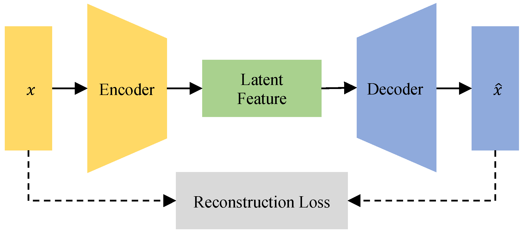
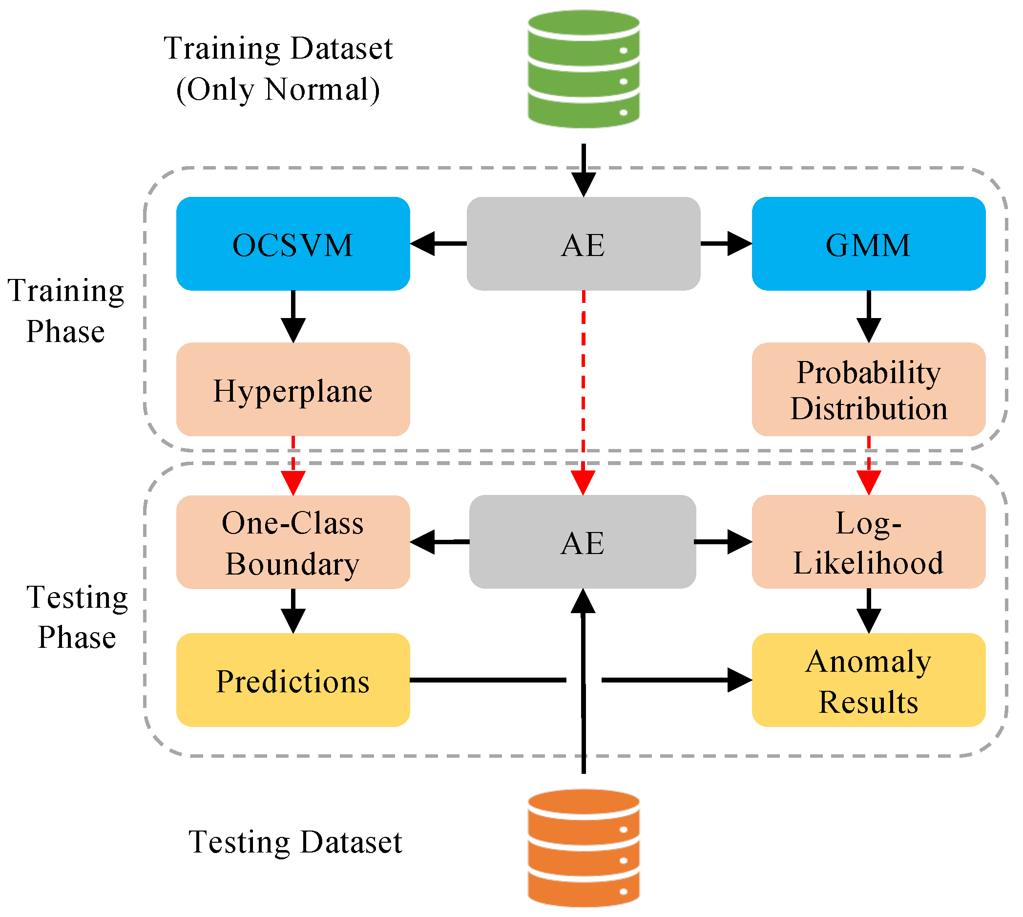
- Before training the anomaly detector, we use the AE to extract representative features from network data. These features are fed into the anomaly detectors. The new features enhance detection performance.
- After obtaining latent features, we employ them to train OCSVM and GMM further. The OCSVM learns a one-class classification boundary; in the meantime, the GMM learns a probability distribution of the normal data. In specifically, the GMM is utilized to reclassify the samples obtained via OCSVM.
- We conduct a number of experiments on two intrusion detection datasets to illustrate their performance. The experiment results indicate that our proposed model demonstrates higher detection capability.
2. Related Work
3. Proposed Methods
3.1. AE
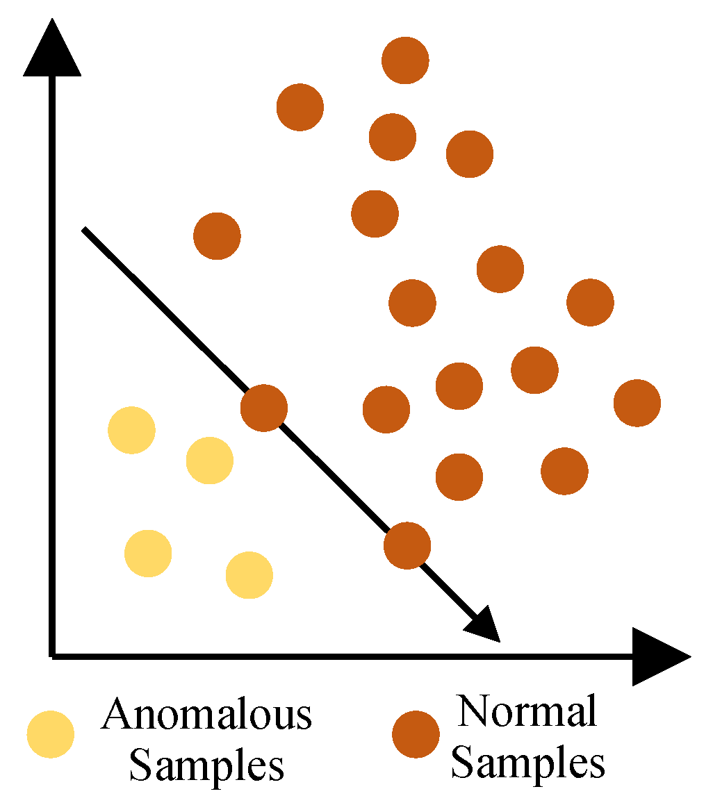
3.2. OCSVM
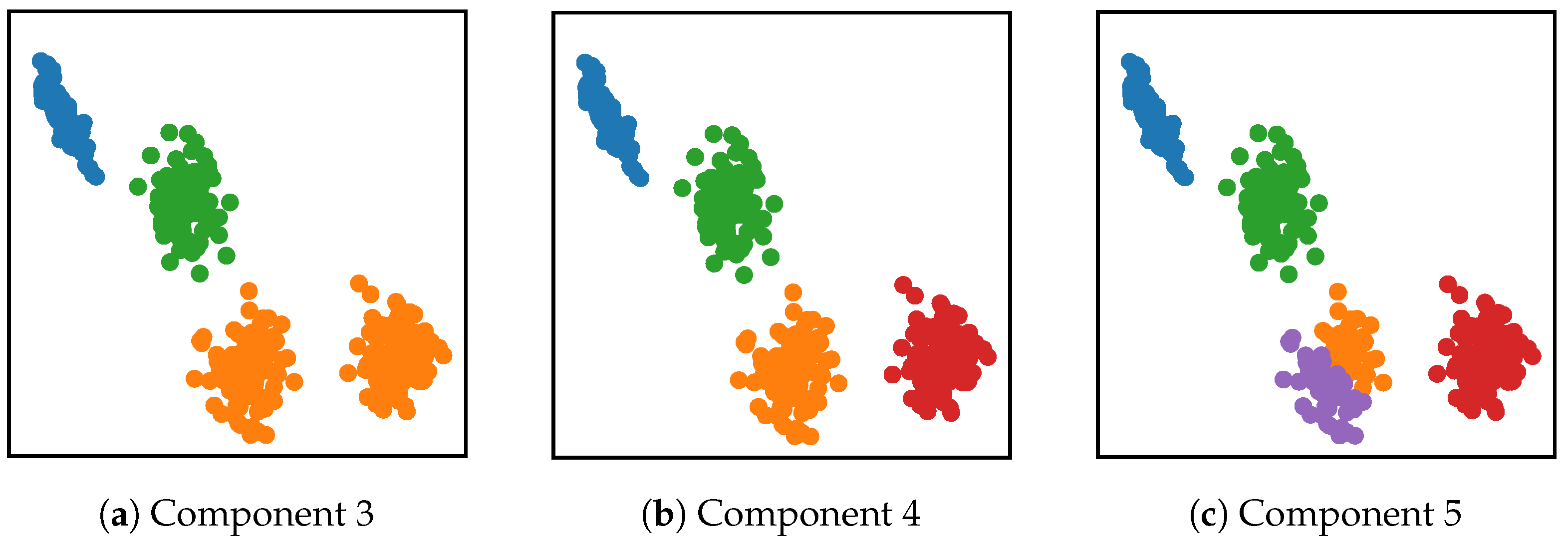
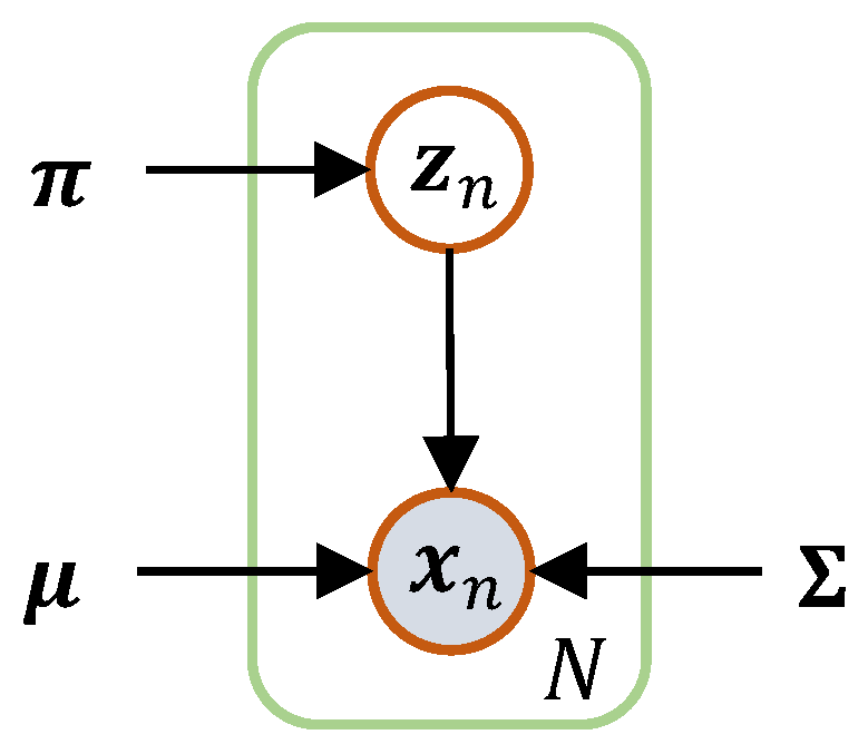
3.3. GMM
3.4. Whole Detection Frame
| Algorithm 1: Testing process of our proposed methods. |
 |
4. Experiment Results
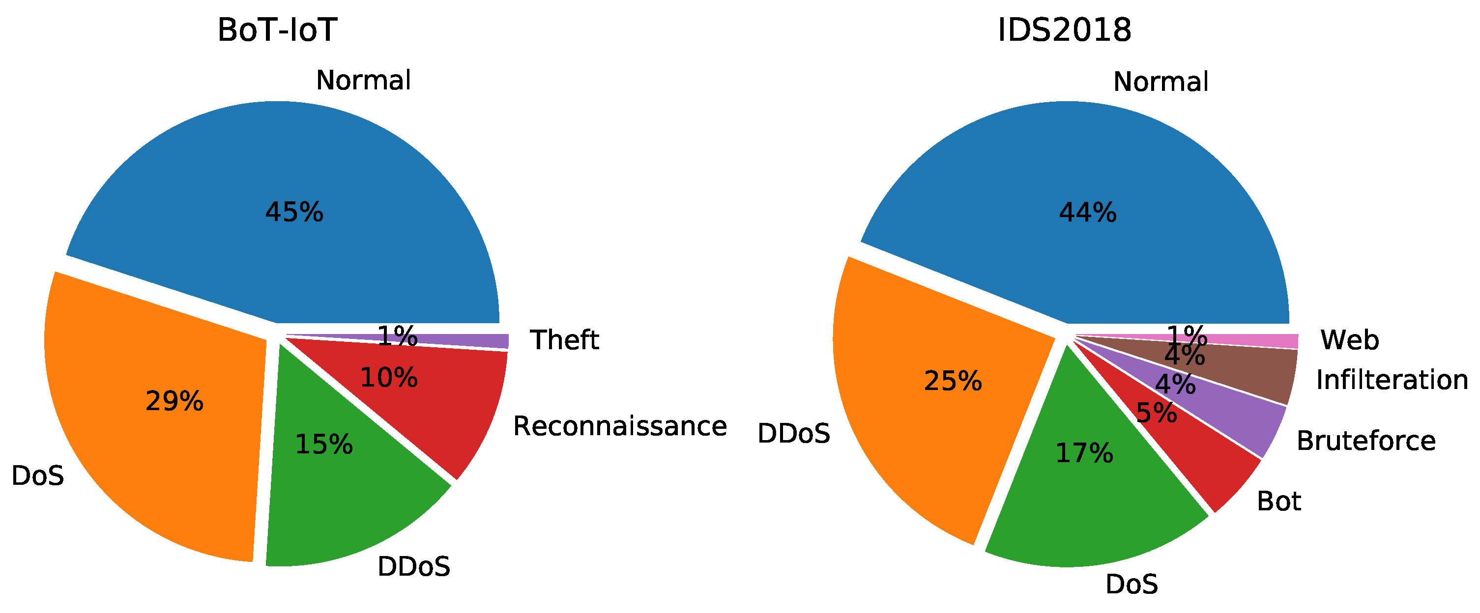
4.1. Dataset
4.2. Evaluation Metric
4.3. Experiment Settings
- IForest. IForest builds numerous isolation trees from random subsets of data and provides an anomaly score by aggregating the results from each tree.
- KDE. KDE is a non-parametric approach to estimate the probability density function using a kernel function. The probability density can be utilized as anomaly score. In this work, we employ the Gaussian kernel.
- Deep support vector data description (DSVDD) [33]. Like OCSVM, the support vector data description (SVDD) is an one-class learning method. It aims to learn the smallest hypersphere that encloses most of the target data. DSVDD utilizes SVDD as a loss function to train the neural network and finds a hypersphere with a minimum volume.
4.4. Experiment Results
4.4.1. Detection Performance
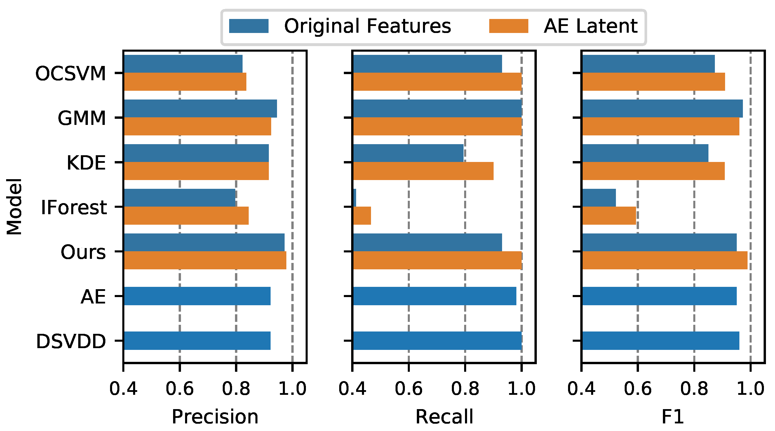
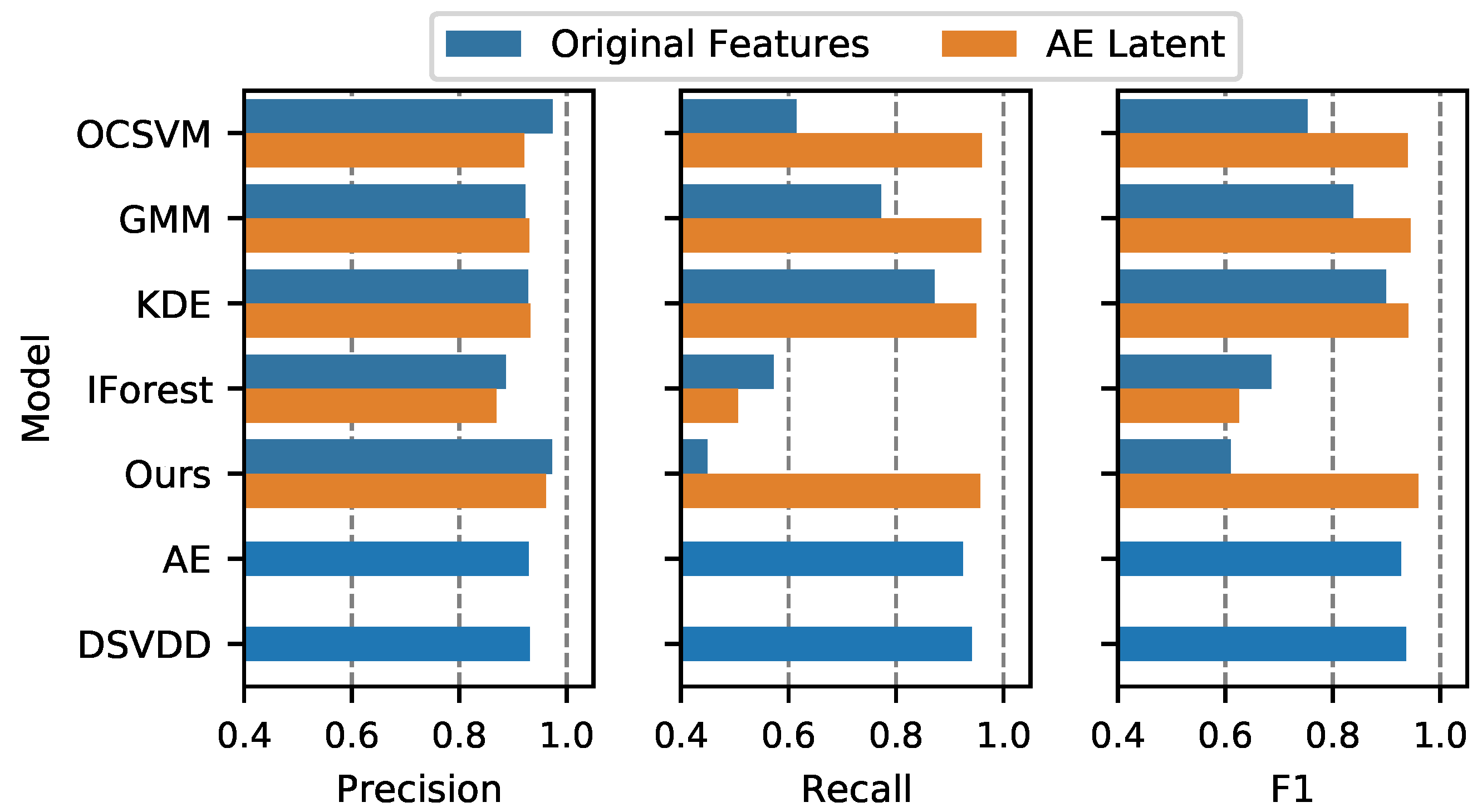
4.4.2. Effect of Feature Extraction by AE
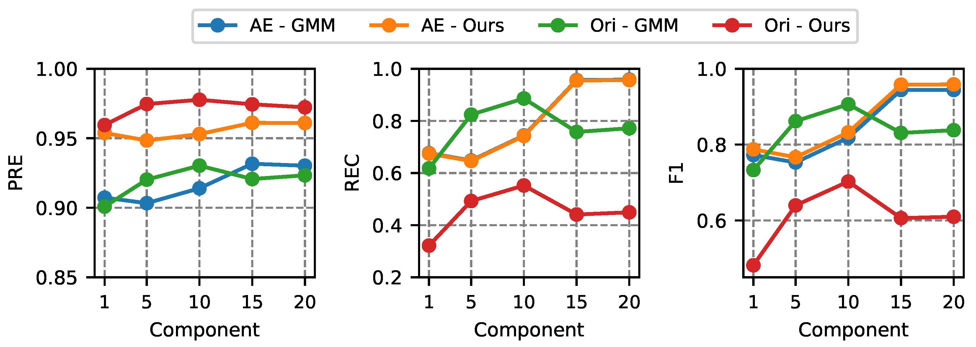
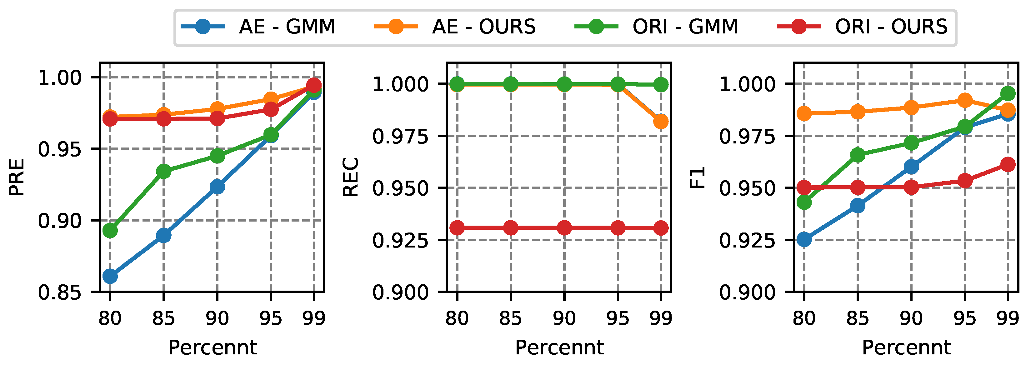
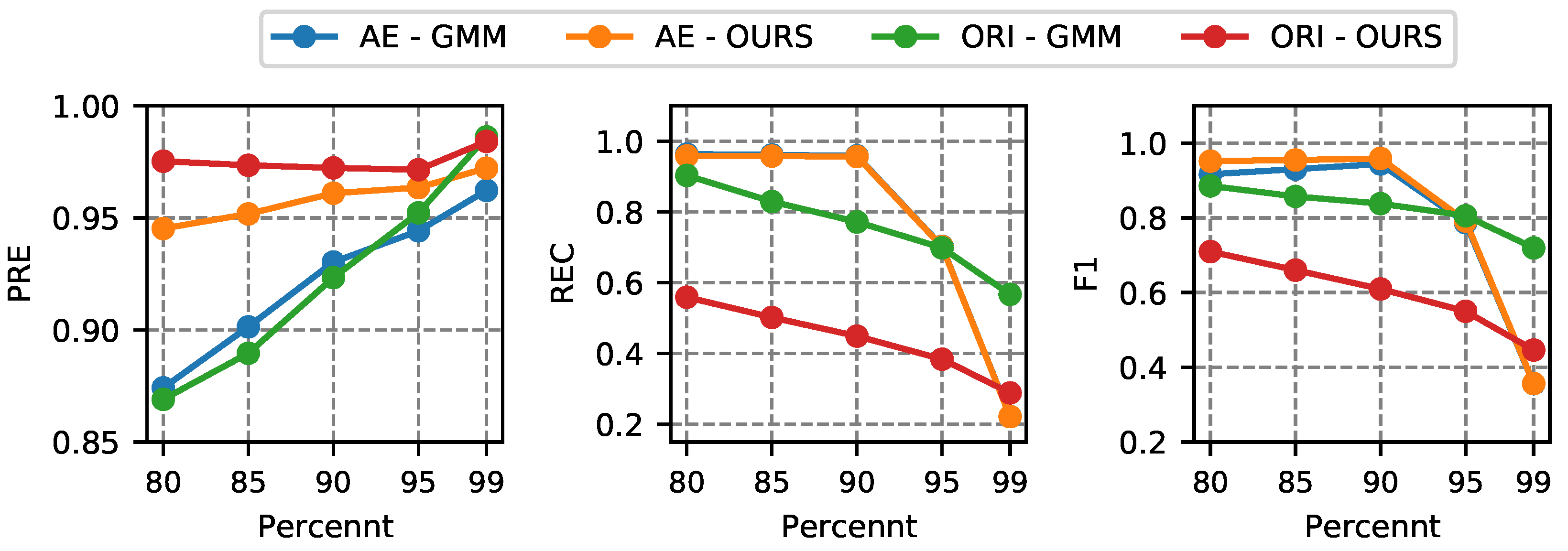
4.4.3. Parameter Analysis
5. Conclusions
Author Contributions
Funding
Data Availability Statement
Conflicts of Interest
References
- Liu, H.; Lang, B. Machine learning and deep learning methods for intrusion detection systems: A survey. Appl. Sci. 2019, 9, 4396. [Google Scholar] [CrossRef]
- Ferrag, M.A.; Maglaras, L.; Ahmim, A.; Derdour, M.; Janicke, H. RDTIDS: Rules and Decision Tree-Based Intrusion Detection System for Internet-of-Things Networks. Future Internet 2020, 12, 44. [Google Scholar] [CrossRef]
- Mohammadi, M.; Rashid, T.A.; Karim, S.H.; Aldalwie, A.H.M.; Tho, Q.T.; Bidaki, M.; Rahmani, A.M.; Hosseinzadeh, M. A comprehensive survey and taxonomy of the SVM-based intrusion detection systems. J. Netw. Comput. Appl. 2021, 178, 102983. [Google Scholar] [CrossRef]
- Bhavani, T.T.; Rao, M.K.; Reddy, A.M. Network Intrusion Detection System Using Random Forest and Decision Tree Machine Learning Techniques. In First International Conference on Sustainable Technologies for Computational Intelligence: Proceedings of ICTSCI 2019; Luhach, A.K., Kosa, J.A., Poonia, R.C., Gao, X.Z., Singh, D., Eds.; Springer: Singapore, 2020; pp. 637–643. [Google Scholar]
- Cao, V.L.; Nicolau, M.; McDermott, J. Learning Neural Representations for Network Anomaly Detection. IEEE Trans. Cybern. 2019, 49, 3074–3087. [Google Scholar] [CrossRef]
- Choi, H.; Kim, M.; Lee, G.; Kim, W. Unsupervised learning approach for network intrusion detection system using autoencoders. J. Supercomput. 2019, 75, 5597–5621. [Google Scholar] [CrossRef]
- Chandola, V.; Banerjee, A.; Kumar, V. Anomaly Detection: A Survey. ACM Comput. Surv. 2009, 14, 1–58. [Google Scholar] [CrossRef]
- Schölkopf, B.; Platt, J.C.; Shawe-Taylor, J.; Smola, A.J.; Williamson, R.C. Estimating the support of a high-dimensional distribution. Neural Comput. 2001, 13, 1443–1471. [Google Scholar] [CrossRef]
- Alazzam, H.; Sharieh, A.; Sabri, K.E. A lightweight intelligent network intrusion detection system using OCSVM and Pigeon inspired optimizer. Appl. Intell. 2022, 52, 3527–3544. [Google Scholar] [CrossRef]
- Al Shorman, A.; Faris, H.; Aljarah, I. Unsupervised intelligent system based on one class support vector machine and Grey Wolf optimization for IoT botnet detection. J. Ambient Intell. Humaniz. Comput. 2020, 11, 2809–2825. [Google Scholar] [CrossRef]
- Cao, V.L.; Nicolau, M.; McDermott, J. A Hybrid Autoencoder and Density Estimation Model for Anomaly Detection. In Parallel Problem Solving from Nature—PPSN XIV; Handl, J., Hart, E., Lewis, P.R., López-Ibáñez, M., Ochoa, G., Paechter, B., Eds.; Springer: Cham, Switzerland, 2016; pp. 717–726. [Google Scholar]
- Vaiyapuri, T.; Binbusayyis, A. Application of deep autoencoder as an one-class classifier for unsupervised network intrusion detection: A comparative evaluation. PeerJ Comput. Sci. 2020, 6, 1–26. [Google Scholar] [CrossRef]
- Blanco, R.; Malagón, P.; Briongos, S.; Moya, J.M. Anomaly Detection Using Gaussian Mixture Probability Model to Implement Intrusion Detection System. In Hybrid Artificial Intelligent Systems; Pérez García, H., Sánchez González, L., Castejón Limas, M., Quintián Pardo, H., Corchado Rodríguez, E., Eds.; Springer: Cham, Switzerland, 2019; pp. 648–659. [Google Scholar]
- Ahmad, Z.; Shahid Khan, A.; Wai Shiang, C.; Abdullah, J.; Ahmad, F. Network intrusion detection system: A systematic study of machine learning and deep learning approaches. Trans. Emerg. Telecommun. Technol. 2021, 32, 1–29. [Google Scholar] [CrossRef]
- Vinayakumar, R.; Alazab, M.; Soman, K.P.; Poornachandran, P.; Al-Nemrat, A.; Venkatraman, S. Deep Learning Approach for Intelligent Intrusion Detection System. IEEE Access 2019, 7, 41525–41550. [Google Scholar] [CrossRef]
- Yang, Y.; Zheng, K.; Wu, C.; Yang, Y. Improving the classification effectiveness of intrusion detection by using improved conditional variational autoencoder and deep neural network. Sensors 2019, 19, 2528. [Google Scholar] [CrossRef]
- Malaiya, R.K.; Kwon, D.; Suh, S.C.; Kim, H.; Kim, I.; Kim, J. An Empirical Evaluation of Deep Learning for Network Anomaly Detection. IEEE Access 2019, 7, 140806–140817. [Google Scholar] [CrossRef]
- Thapa, N.; Liu, Z.; Kc, D.B.; Gokaraju, B.; Roy, K. Comparison of machine learning and deep learning models for network intrusion detection systems. Future Internet 2020, 12, 167. [Google Scholar] [CrossRef]
- Alzubaidi, L.; Zhang, J.; Humaidi, A.J.; Al-Dujaili, A.; Duan, Y.; Al-Shamma, O.; Santamaría, J.; Fadhel, M.A.; Al-Amidie, M.; Farhan, L. Review of Deep Learning: Concepts, CNN Architectures, Challenges, Applications, Future Directions. J. Big Data 2021, 8, 53. [Google Scholar] [CrossRef]
- Abdelmoumin, G.; Whitaker, J.; Rawat, D.B.; Rahman, A. A Survey on Data-Driven Learning for Intelligent Network Intrusion Detection Systems. Electronics 2022, 11, 213. [Google Scholar] [CrossRef]
- Fu, Y.; Du, Y.; Cao, Z.; Li, Q.; Xiang, W. A Deep Learning Model for Network Intrusion Detection with Imbalanced Data. Electronics 2022, 11, 898. [Google Scholar] [CrossRef]
- Abdulhammed, R.; Musafer, H.; Alessa, A.; Faezipour, M.; Abuzneid, A. Features dimensionality reduction approaches for machine learning based network intrusion detection. Electronics 2019, 8, 322. [Google Scholar] [CrossRef]
- Qi, R.; Rasband, C.; Zheng, J.; Longoria, R. Detecting cyber attacks in smart grids using semi-supervised anomaly detection and deep representation learning. Information 2021, 12, 328. [Google Scholar] [CrossRef]
- Sadaf, K.; Sultana, J. Intrusion detection based on autoencoder and isolation forest in fog computing. IEEE Access 2020, 8, 167059–167068. [Google Scholar] [CrossRef]
- Yan, W. Detecting Gas Turbine Combustor Anomalies Using Semi-Supervised Anomaly Detection with Deep Representation Learning. Cogn. Comput. 2020, 12, 398–411. [Google Scholar] [CrossRef]
- Liao, J.; Teo, S.G.; Pratim Kundu, P.; Truong-Huu, T. ENAD: An ensemble framework for unsupervised network anomaly detection. In Proceedings of the 2021 IEEE International Conference on Cyber Security and Resilience (CSR), Rhodes, Greece, 26–28 July 2021; pp. 81–88. [Google Scholar]
- Géron, A. Hands-On Machine Learning with Scikit-Learn, Keras, and TensorFlow; O’Reilly Media, Inc.: Sebastopol, CA, USA, 2022. [Google Scholar]
- Beggel, L.; Pfeiffer, M.; Bischl, B. Robust Anomaly Detection in Images Using Adversarial Autoencoders. In Proceedings of the Machine Learning and Knowledge Discovery in Databases; Brefeld, U., Fromont, E., Hotho, A., Knobbe, A., Maathuis, M., Robardet, C., Eds.; Springer International Publishing: Cham, Switzerland, 2020; pp. 206–222. [Google Scholar]
- Seliya, N.; Abdollah Zadeh, A.; Khoshgoftaar, T.M. A Literature Review on One-Class Classification and Its Potential Applications in Big Data. J. Big Data 2021, 8, 122. [Google Scholar] [CrossRef]
- Bishop, C.M.; Nasrabadi, N.M. Pattern Recognition and Machine Learning; Springer: New York, NY, USA, 2006; Volume 4. [Google Scholar]
- Aggarwal, C.C. Outlier Analysis; Springer: New York, NY, USA, 2013; pp. 1–446. [Google Scholar]
- Sarhan, M.; Layeghy, S.; Portmann, M. Towards a Standard Feature Set for Network Intrusion Detection System Datasets. Mob. Netw. Appl. 2021, 27, 357–370. [Google Scholar] [CrossRef]
- Ruff, L.; Vandermeulen, R.; Goernitz, N.; Deecke, L.; Siddiqui, S.A.; Binder, A.; Müller, E.; Kloft, M. Deep One-Class Classification. In Proceedings of the 35th International Conference on Machine Learning, Stockholm, Sweden, 10–15 July 2018; pp. 4393–4402. [Google Scholar]
- Pedregosa, F.; Varoquaux, G.; Gramfort, A.; Michel, V.; Thirion, B.; Grisel, O.; Blondel, M.; Prettenhofer, P.; Weiss, R.; Dubourg, V.; et al. Scikit-learn: Machine learning in Python. J. Mach. Learn. Res. 2011, 12, 2825–2830. [Google Scholar]
- Keras. 2015. Available online: https://keras.io (accessed on 10 February 2023).
- He, K.; Zhang, X.; Ren, S.; Sun, J. Delving deep into rectifiers: Surpassing human-level performance on imagenet classification. In Proceedings of the 2015 IEEE International Conference on Computer Vision (ICCV), Santiago, Chile, 7–13 December 2015; pp. 1026–1034. [Google Scholar]


| Actual Condition | Predicted Condition | |
|---|---|---|
| Attack | Normal | |
| Attack | True Positive | False Negative |
| Normal | False Positive | True Negative |
| Method | Accuracy | Precision | Recall | F1 | FPR |
|---|---|---|---|---|---|
| IForest | |||||
| KDE | |||||
| GMM | |||||
| OCSVM | |||||
| AE | |||||
| DSVDD | |||||
| Ours |
| Method | Accuracy | Precision | Recall | F1 | FPR |
|---|---|---|---|---|---|
| IForest | |||||
| KDE | |||||
| GMM | |||||
| OCSVM | |||||
| AE | |||||
| DSVDD | |||||
| Ours |
Disclaimer/Publisher’s Note: The statements, opinions and data contained in all publications are solely those of the individual author(s) and contributor(s) and not of MDPI and/or the editor(s). MDPI and/or the editor(s) disclaim responsibility for any injury to people or property resulting from any ideas, methods, instructions or products referred to in the content. |
© 2023 by the authors. Licensee MDPI, Basel, Switzerland. This article is an open access article distributed under the terms and conditions of the Creative Commons Attribution (CC BY) license (https://creativecommons.org/licenses/by/4.0/).
Share and Cite
Wang, C.; Sun, Y.; Lv, S.; Wang, C.; Liu, H.; Wang, B. Intrusion Detection System Based on One-Class Support Vector Machine and Gaussian Mixture Model. Electronics 2023, 12, 930. https://doi.org/10.3390/electronics12040930
Wang C, Sun Y, Lv S, Wang C, Liu H, Wang B. Intrusion Detection System Based on One-Class Support Vector Machine and Gaussian Mixture Model. Electronics. 2023; 12(4):930. https://doi.org/10.3390/electronics12040930
Chicago/Turabian StyleWang, Chao, Yunxiao Sun, Sicai Lv, Chonghua Wang, Hongri Liu, and Bailing Wang. 2023. "Intrusion Detection System Based on One-Class Support Vector Machine and Gaussian Mixture Model" Electronics 12, no. 4: 930. https://doi.org/10.3390/electronics12040930