1. Introduction
Direction-of-arrival (DOA) estimation is an essential task in array signal processing due to the extensive applications in radar, wireless communications, and acoustics [
1]. Model-based DOA estimation approaches have been comprehensively investigated, including Fourier Transform (FT), subspace methods, and compressed sensing (CS) [
2]. FT is easy to implement with high computational efficiency and robustness [
3]. However, its angular resolution is restricted by the size of the array. Subspace methods, such as multiple signal classification (MUSIC) [
4] and estimation of signal parameters via rotational invariance techniques (ESPRIT) [
5], can break the resolution barrier. They utilize the orthogonality between the signal subspace and the noise subspace, which usually requires multiple snapshots to estimate the covariance matrix and the underlying subspaces [
6]. CS methods solve the angular observation equation by introducing certain sparse regularizations such as L
0 or L
1-norm [
7,
8]. The accuracy and resolution are improved at a much higher computational cost [
9].
Despite the wide applications, model-based approaches are susceptible to adverse conditions, such as low signal-to-noise ratio (SNR) and array imperfections. Recently, owing to the powerful nonlinear fitting capabilities, deep neural network (DNN) has been introduced to DOA estimation [
10,
11]. As a data-driven approach, DNN can deal with adverse situations given sufficient training samples. The key concept of existing DNN methods is discretizing the field of view (FOV) and transforming DOA estimation into a multi-label classification task. To cope with the low SNR conditions, the networks are trained across a range of low SNRs and outperform their competitors in the low SNR regime [
12,
13]. To obtain good adaptation to array imperfections, autoencoders are constructed to reduce the influence of noise and array imperfections, after which the network performs satisfyingly in imperfection adaptation [
14]. In addition, a new deep learning architecture is proposed based on the imperfect array, and the output of the network is a vector for the spectrum estimation, which can avoid discretizing the spatial domain [
15]. Furthermore, to deal with the grid mismatch, some networks are proposed to exploit the Toeplitz property and reconstruct the covariance matrix, and model-based approaches, such as MUSIC or root-MUSIC, are applied to obtain gridless DOA [
16,
17].
DNN has shown great potential in adverse conditions. However, high dynamic SNR is still a limiting factor in the accuracy of DOA estimation. DNN requires enough training samples that cover all the practical situations. When the number of sources is large, it is difficult to cover all possible combinations of positions and amplitudes. When the SNRs of the sources vary significantly, weaker sources achieve much lower accuracy or may even be missed. Moreover, the number of sources is usually needed as the prior information. The number of the resulting training samples is huge, which leads to very high computational costs as well [
13].
In this paper, we propose a DNN framework with a sliding window (DNN-SW) for DOA estimation to cope with the high dynamic SNR scenarios. The entire FOV is divided into a series of overlapping angular sub-regions through the sliding window operation. The core network consists of a detector network and an estimator network. The detector determines whether the sub-region contains a source, and the estimator informs its angle. This paper assumes that there is only one source in each sub-region. Based on the assumption, single-source data is used to train the networks, and the requirement of the training sample is alleviated. Compared with existing methods based on DNN, the DOA estimation task is jointly accomplished by multiple networks, and each network only estimates the angle of the current sub-region, greatly simplifying the task of each network and improving network performance in high dynamic scenarios. Furthermore, the number of sources can be obtained adaptively according to the number of sub-regions in which the source exists, which adapts to the number of sources.
The rest of the paper is organized as follows. In
Section 2, we present the signal model. In
Section 3, we introduce the input data preprocessing and network structure in detail, including the sliding window module, detection module, DOA estimation module, and angle merging. In
Section 4, we offer the results of the simulation to prove the advantageous performance of the proposed method by comparing the other approaches and collecting the real data for verification. Finally, conclusions are summarized in
Section 5.
2. Signal Model
In this paper, the single snapshot scenario is considered [
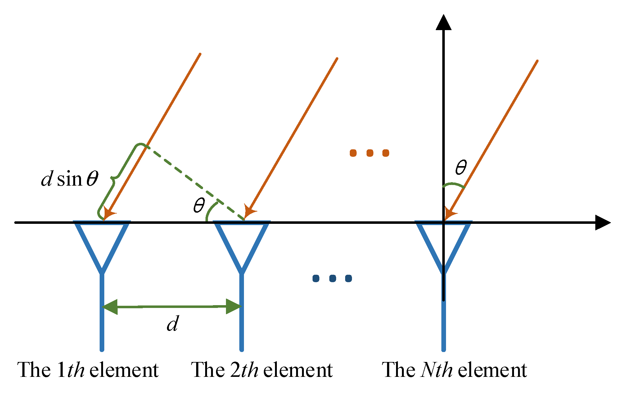
18]. As shown in
Figure 1, we consider a uniform line array (ULA) with
N elements in the narrow-band mode. It is assumed that there are
K far-field sources from
,
indicates the direction of the
kth source, and the received signal can be formulated as
where
represents the amplitude of the sources and
is a
vector denoting the statistically independent white Gaussian noise vector with zero mean value and unknown variance
. The steering vector
can be expressed as
where
is the wavelength of the transmitted signal,
f is the carrier frequency and
c is the speed of the light. Additionally,
d describes the array element space. As for
A(θ), it is the array manifold matrix, which can be written as
3. The Proposed Method
The structure of DNN-SW is shown in
Figure 2. it is divided into several overlapping sub-regions and assume the sources are located in different sub-regions independently. Specifically, there are four main modules in the proposed network. First, in the sliding window module, the FOV is split into a series of overlapping sub-regions in which there is one source at most. Then, the detection module and DOA estimation module are followed. The detection module contains multiple detectors for each sub-region. The detector network determines whether a source exists in the corresponding sub-region, which is formed as a binary classification task. Similar to the detection module, the estimation module also includes multiple estimator networks to obtain the angles of the sources. Since the sub-regions are overlapped, one source can be detected and estimated in several sub-regions. Therefore, an angle merging module is applied to give the final results.
3.1. Input Data Preprocessing
To retain the amplitude and phase information of the single snapshot signal
x [
19], we extract four parts of information from
x, including the real part, imaginary part, angle value, and modulus. The input vector
X can be described as
3.2. Sliding Window Module
To alleviate the negative influence of different sources in the high dynamic SNR scenario, the sliding window module is proposed. By detecting and estimating the sources separately through the network, the information of each source can be focused on and easily extracted. Furthermore, based on this structure, the detectors and estimators are trained using single-source data. Compared to other methods [
11,
12,
13,
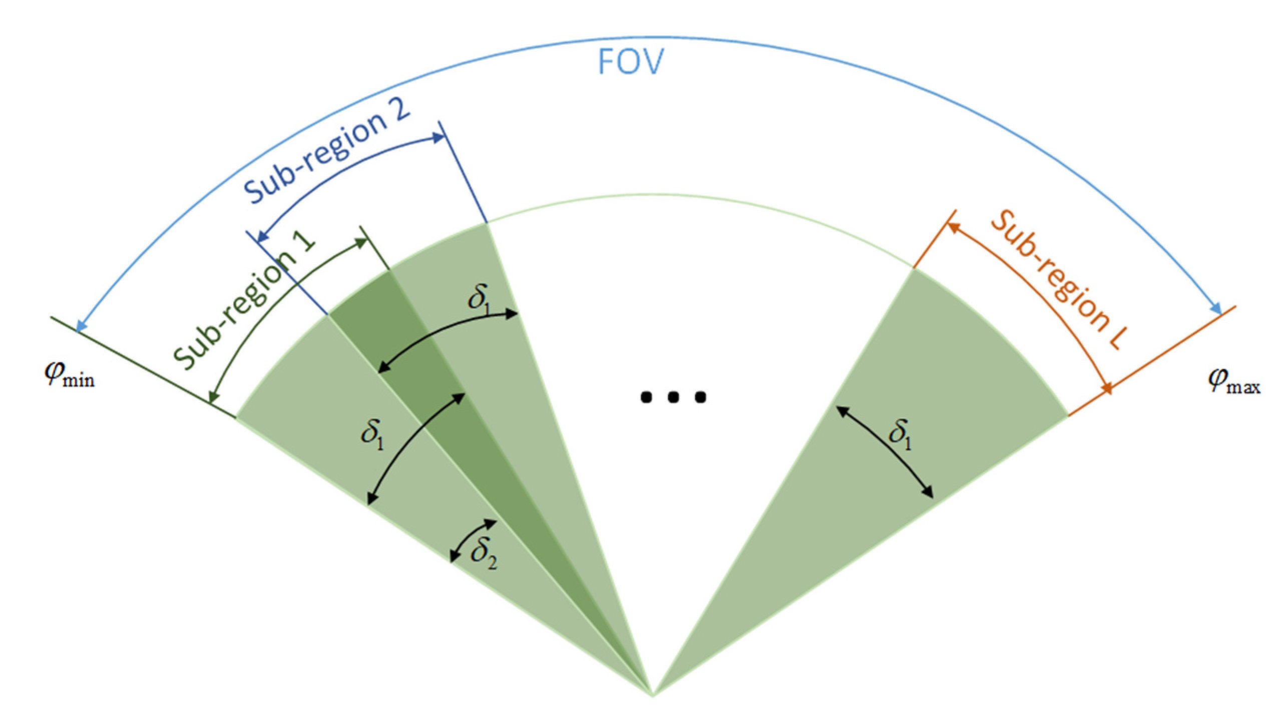
14], we can greatly reduce the number of training samples and the training time cost. Here, the range of the FOV is
, it is divided into several overlapping sub-regions, as shown in
Figure 3. In this paper, the range of the sub-region
δ1 is set to be close to
(the 3 dB beamwidth of the array), resulting in the situation that at most one source can be estimated in each sub-region. According to [
20],
can be calculated by
where,
is the center of the beamwidth. Moreover,
is the step size when dividing the FOV. To alleviate the missing problem of sources and improve the estimation accuracy, each source is set in multiple sub-regions for repeated detection and estimation, resulting in
. Thus, in this paper,
is configurated to be
, and the number of sub-regions
L is
3.3. Detection Module
The structure of this module is shown in
Figure 2.
L detector networks are constructed to accomplish the detection task in
L sub-regions. The data is fed into the
L detectors to decide which sub-regions the sources are located in. Since this is a supervised task, the training and testing details are introduced, respectively. During the training process, take the
ith detector as an example; given the
jth training data
, the output
can be obtained
where
f1 to
fW are
W fully connected layers.
f1 to
fW−1 are all followed by a rectified linear unit (ReLU) layer. Finally, the Tanh layer is applied to generate the final detection. The ReLU layer and Tanh layer are defined as
Furthermore,
represents the ground-truth label of the sample
. If
is in the
ith sub-region, the label
is set to 1; otherwise,
is set to 0. For each detector, the mean square error is served as the loss function for backpropagation to evaluate the detection performance. The objective function can be written as
where
J denotes the number of all the training samples. The parameters of the network are updated by minimizing (10) through the adaptive moment estimation (Adam) optimizer.
In the testing process, a threshold
Th1 is designed to judge whether the source lies in
ith sub-region. Its value is determined by the statistical analysis results of training samples to guarantee a satisfying detection. The details will be discussed in the simulation section. When a testing sample
is put into the
ith detector,
is the detection result, which is defined as
When , the source is considered in this sub-region, otherwise, it does not exist in this sub-region.
3.4. DOA Estimation Module
After detecting which sub-regions the sources are in, the DOA estimation module is built to achieve the specific angle estimation task. As shown in
Figure 2, similar to the detection module,
L estimator networks are established for the
L sub-regions. For each estimator, the sub-region is further divided into a series of grids with the step of
δ3 and the number of grids
M is
. During the training process, to avoid the negative effects of error detection, estimators are trained independently of the detectors. We take the
ith estimator into account, given the sample
, the input data of this estimator is
, which means only the data in the
ith sub-region is trained. In the estimating phase, the label is encoded by the one-hot encoding method, which is a vector that represents the probabilities of all the alternative angles. The ground-truth label
of
for the
ith estimator can be written as
. If the source locates in the
mth grid,
is 1, otherwise,
is 0. When training, the estimation results of the estimator
can be expressed as
where
to
are
Z fully connected layers.
to
are followed by a ReLU layer and
is followed by a Softmax layer. The Softmax layer is defined as
According to the ground-truth label
and the predicted label
, cross-entropy is selected as the loss function
where
J denotes the number of training samples. The parameters of the estimator are updated by minimizing (14) through the Adam optimizer.
In the testing process, for the
ith estimator, the sample
is served as the input data based on the detection result. The input can be formulated as
. Only when
is 1, does the output of the estimator makes sense. The location with max probability is used to calculate the estimated angle
, and it can be expressed as
3.5. Angle Merging
Through the detection and DOA estimation module, the source is first detected, and then the specific angle is obtained. However, although the adjacent overlapping sub-regions allow the detection results to be more accurate and complete, the same source will be detected and estimated repeatedly in multiple sub-regions. Namely, several angles may be obtained according to one source. An angle merging algorithm is proposed to solve the angle redundancy problem. The estimated angles from the same source are considered to have minor differences so that they can merge into one angle as the final output. The fusion threshold
Th2 is introduced to decide whether the angles should be fused. Since high-resolution DOA estimation is not considered in this paper,
Th2 is set to be a little lower than
. If the difference between the estimated angles
is lower than
Th2, they will be merged by
After the merging algorithm, the final angles estimated are obtained, and the number of sources can be acquired automatically.
4. Experiment
In this section, we conduct the DOA estimation based on the simulation data and real data to evaluate the proposed method. First, the simulation data is used to verify the effectiveness and advantages of our method. Then, we collected real radar signals to assess the performance of DNN-SW in practical application.
4.1. Simulation Settings
In the simulations, the FOV is the range of
, and a 40-element uniform linear array with
inter-element spacing is considered. According to (5), since the
of different beamwidth centers are different, in this paper, the center of FOV is set as the beamwidth center
. When
is 30°,
is 3.01°. The range of sub-region
δ1 is set to 3° and the step size
δ2 is set to 1.5°. As a result, the sub-region number
L is 79. Additionally, the sampling interval
δ3 is specified as 0.1° so that the grid number for each sub-region
M is 30 and the grid number for FOV is 1200 categories of direction in total. The detailed parameters are listed in
Table 1.
For the training dataset, the SNR of the source is 15 dB, and 30 samples are collected in each direction. Therefore, there are 36,000 training samples in total. For each detector and estimator, the size of training data is 36,000 and 900, respectively. For all the experiments, the SNR is defined in [
13]
where
represents the power of the
ith source,
.
represents the power of the noise.
For each detector, the number of neurons per layer of the network is {16, 1} with a batch size of 128 during 100 training epochs. Similarly, for each estimator, the number of neurons per layer of the network is {128, 256, 30} with a batch size of 128 during 200 training epochs. Moreover, the learning rate is configured to 0.001 for all networks.
The simulations are carried out in a workstation with MATLAB R2022a, Intel Xeon Gold 6240 processor at 2.60GHz, and NVIDIA A100 Tensor Core GPU. The detector networks and estimator networks are based on Pytorch 1.11.0 and Python 3.9.12. Based on the conditions in the training process, the average running time of all the 79 detection networks and estimator networks is about 90.2 s and 5.6 s, respectively. In the testing process, each detection network and each estimator network respectively cost 3.09 us and 3.89 us, which is obtained by calculating the average running time of 1000 testing samples.
4.2. Evaluation Metrics
In the simulations, to objectively and effectively evaluate the performance of the DNN-SW, two evaluation metrics are utilized, including Acc and root mean square error (RMSE). Since the number of sources is unknown, Acc is an important metric to evaluate DNN-SW. It describes the percentage of the number of testing samples whose source numbers are estimated correctly by the network [
21]. It can be formulated as
where
Here, and denotes the ground truth and the prediction directions of the ith testing sample, respectively, , where m denotes the number of testing samples.
Additionally, RMSE is also a classic and common metric in past research [
13,
22]. We calculate the RMSE of the testing samples whose source number is estimated correctly. RMSE can be obtained by
where
H represents the number of samples whose source number is estimated correctly, and
Q represents the number of the source in a testing sample.
and
denote the
qth estimated direction and ground-truth direction of the
hth sample, respectively.
4.3. Determination of Th1 and Th2
In this part, the determination methods of
and
are described in detail. Since the detection process can be regarded as a binary task and
is an important threshold to decide the detection results,
F1 score is served as the criterion to select the optimal parameter
. In binary classification tasks, the
F1 score is widely used to analyze the accuracy of machine learning models [
23,
24,
25,
26]. It takes both the
precision and
recall of the model into account to provide an objective description of the method.
In order to obtain the
F1 score for the detector network, the samples can be split into four parts according to their ground truth and predicted labels, as shown in
Table 2.
In the detector network, the sample is considered positive if its source is in the corresponding sub-region. According to [
25],
precision and
recall are first calculated by
where
precision is the proportion of the positive predicted samples in the actual positive samples, and
recall is the proportion of the actual positive samples in all predicted positive samples. It should be noted that since there are
L = 79 detectors in our method, the number of samples used to obtain the
precision and
recall are the overall number of samples of all 79 detectors. In this case, the overall performance of the detection module is assessed, and the results will not be influenced by the extreme results of some detectors. Then,
score is obtained by calculating the harmonic mean of
precision and
recall
where the range of
is
. If all the positive samples are wrongly predicted,
is equal to 0 which is the minimum value. Additionally, when the samples are all correctly predicted,
is equal to 1, which is the maximum value.
In the simulation, to select the best threshold
, we randomly generate 10,000 testing samples. The samples contain two sources, which are not located in one sub-region, and the SNR of these sources is configured to 15 dB. According to (23), we calculate the
for each
with the step of 0.05 from 0 to 1, and the results are shown in
Figure 4.
From
Figure 4, we can observe that the
score increases and then decreases with the increase of
. When
is 0.25,
reaches the highest, which is 0.942. Thus, the
is fixed to 0.25 in the remaining simulations and real data experiments.
As for the threshold of angle merging , since the high-resolution DOA estimation is not considered, it is supposed to be lower than . Therefore, is set to 2° in the simulation and real data experiments.
4.4. Simulation Results
4.4.1. Sources in the Same SNR Scenarios
Two simulations are conducted under adverse conditions to assess the performance of DNN-SW, including low SNR and array imperfections. In this part, the high dynamic condition is not considered, which means that the SNR of all the sources is the same.
Since the DNN-SW can estimate the number and directions of sources simultaneously, in this simulation, the two values are unknown, and both need to be obtained. To further evaluate the proposed method, the comparison methods are applied. The existing methods can rarely achieve the two tasks at the same time. Therefore, the whole task is divided into the source number estimation part and the DOA estimation part for the comparison methods. In the source number estimation part, two conventional methods are employed for comparison, including AIC and MDL [
27,
28,
29,
30,
31]. Then, in the DOA estimation part, FFT, MUSIC, and ESPRIT are utilized. Furthermore, since MUSIC and ESPRIT are based on the covariance matrix, the space smoothing algorithm is applied to generate the covariance matrix before estimation [
32].
Firstly, we consider two sources in the low SNR situation, and both targets have the same SNR in the testing sample. Two sources impinge on this array from the directions of −6.25° and 3.18°. The SNR varies from 0 dB to 20 dB with the step of 2 dB. For each SNR, the RMSE is obtained by averaging the results of 1000 Monte Carlo (MC) runs. The source number estimation and DOA estimation results are shown in
Figure 5, respectively. In (a), we can observe that the Acc of three source number estimation methods all reach very high. For MDL and DNN-SW, when SNR is larger than 4 dB, the Acc is constantly above 99.5%. For AIC, the Acc is a little lower, which is about 98%, while it is more robust to SNR. The results indicate that the proposed method can achieve advanced performance for source number estimation. Furthermore, considering AIC is more robust and the difference of RMSE based on the two methods is small due to the high Acc, and adequate MC runs, the results of AIC are used to accomplish DOA estimation for FFT, MUSIC, and ESPRIT. As for the DOA estimation results in (b), the results show that as the SNR increases, the RMSE of all methods decreases. Among all the methods, DNN-SW performs best when SNR is below 18 dB. The results indicate that compared with other methods, DNN-SW can achieve better DOA estimation performance in low SNR conditions due to its strong data-fitting capability.
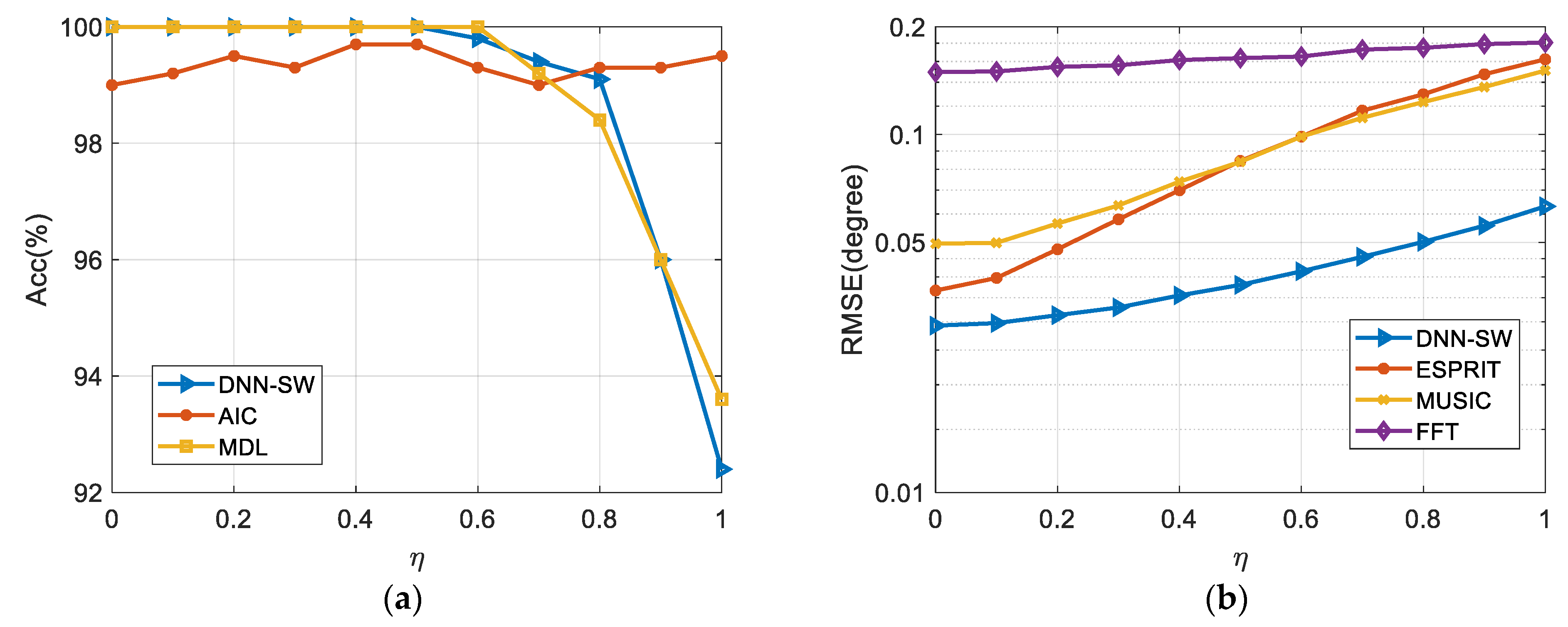
Moreover, three kinds of array imperfections are considered, including gain inconsistent, phase inconsistent, and position perturbation [
14]. It is assumed that the gain-phase inconsistency and position perturbation of different antennas are uniformly distributed within 3
η dB, 30
η°, and 0.15
λη, respectively.
η is an imperfect factor to measure the imperfect effect, and it varies from 0 to 1 with the step of 0.1. In this simulation, two sources impinge on this array from the directions of −6.25° and 3.18°. The SNR of these sources is set to 15 dB. For each
η, the RMSE is obtained by averaging the results of 1000 MC runs. The results are shown in
Figure 6. From (a), it can be observed that the three methods can all estimate the source number accurately. The Acc of DNN-SW is above 99% when
η is 0.8 and can reach 92% even
η is 1, which means the source number estimation results of DNN-SW are reliable. For MDL and AIC, the results are both satisfying, and they show a similar law to the previous simulation. In this case, the number estimation results of AIC are still considered the basis for DOA estimation comparison methods. (b) gives the RMSE of different methods, and DNN-SW consistently performs better than other methods when the error increases. The results show that the deep learning method is more robust for array imperfections because it has the capability of adaptively learning detailed information from the input data.
4.4.2. Sources in High Dynamic SNR Scenarios
In this part, we focus on the high dynamic SNR scenarios, which means the SNRs of different sources are different. Since the results in
Section 4.4.1 show that the deep learning methods perform better under adverse conditions than conventional methods, in this simulation, two deep learning methods for DOA estimation are applied as comparisons, including DNN-NSW and Deep convolution network (DCN) [
11]. The difference between DNN-NSW and DNN-SW is that there is no overlapping part between adjacent sub-regions in DNN-NSW. That is to say, in DNN-NSW, the step size of the sliding window
is set to 3°, which is the same as the
. So, a source will only appear in one sub-region. The remaining parameters and configurations of the two methods are the same. Furthermore, due to DCN methods needing multiple snapshots, the number of snapshots is set to 50.
Firstly, we change the directions of the two sources to assess the DOA estimation performance. The first source
varies from −49.59° to 49.41° with the step of 1°, and the direction of the second source
is set to
. The directions of the sources are all off-grid. When the SNR of the two sources is both 10 dB, the estimation results of DCN and DNN-SW are shown in
Figure 7a, b, and c, respectively. We can observe that the three deep learning methods can achieve satisfying performance in the ideal case.
Figure 7d–f depicts the results when the SNRs of two sources are 10 dB and 18 dB, respectively. The results demonstrate that ΔSNR between two sources severely degrades the performance of DCN; the source with lower SNR is rarely estimated. By contrast, DNN-SW can significantly alleviate the problem due to the design of the sub-region network structure. The lower SNR source is estimated in its sub-region, and the influence of the other sources can be reduced. In addition, compared with DNN-NSW, we can infer that the sliding window can improve the accuracy of estimating the number of sources and the performance of DOA estimation.
Additionally, to investigate the effect of the difference of SNRs between two sources, the direction of the two sources is fixed at 6.28° and 15.72°, and the SNR of the sources are configured as 10 dB and 10 dB + ΔSNR, respectively. In the simulation, ΔSNR varies from 0 dB to 10 dB, and the RMSE for each ΔSNR is obtained by calculating the average results of 1000 MC runs. As shown in
Figure 7d, since DCN may miss the low SNR source, the Acc of three methods is also discussed. The results are shown in
Figure 8a; it can be seen that DNN-SW can precisely estimate the source number even for high ΔSNR, while DCN fails to estimate the source number when ΔSNR > 5 dB. As for the RMSE given in
Figure 8b, it can be observed that the RMSE of DNN-SW is much lower than DNN-NSW due to the overlapping design and repeat estimation of the sources. As for DCN, it achieves a more precise estimation when ΔSNR is small because the input contains information from multiple snapshots. However, with the increase of ΔSNR, DNN-SW shows its advantages due to the design of the sub-region network structure.
4.5. Real Data Experiment Results
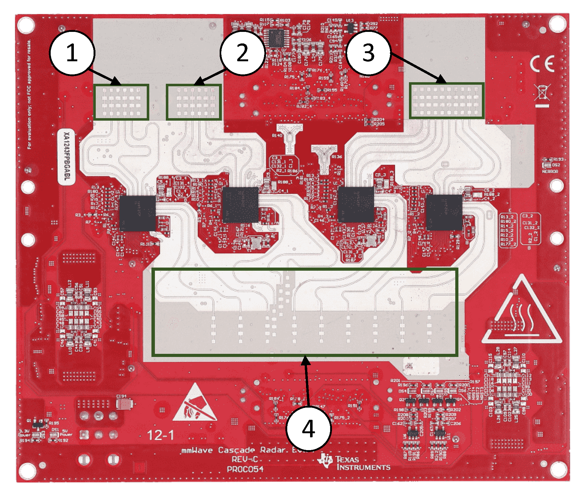
To further evaluate the practical application value of DNN-SW, the real data are collected using MMWCAS-RF-EVM radar in the practical scenario, and the experiments are conducted based on the real data. The specific configurations of the radar antennas are described
Figure 9. It has 12-transmit and 16-receive antennas, resulting in 86 non-overlapping azimuth virtual arrays. In this experiment, there are 40 virtual arrays considered. The data collection scenario is shown in
Figure 10. Two different corner reflectors are fixed at a distance of 6 m from the radar, and their directions relative to the radar are −7.2° and 4.8°, respectively. In [
13], the RMSE of ESPRIT is lower than 0.01 when the array element is 16, the number of snapshots is 1000, and the SNR of sources is 15 dB. Based on this result, in our experimental condition, the ground-truth directions of the corner reflectors are calculated using 86 virtual arrays and 1000 snapshots by the ESPRIT methods, and the RMSE will be lower than 0.01. Therefore, it is considered the ground truth in this real data experiment.
Based on the measured reflected signal, the DOA estimation results of four methods are shown in
Figure 11 and
Table 3. We can observe from the spectrum in
Figure 11 that the difference in the SNR of the two corner reflectors is 5.3 dB. In this case, DNN-SW performs best whose RMSE is only 0.071. For the conventional methods, the estimation error is larger, and MUSIC performs best among them. As for the deep learning method, DCN, the higher source is estimated more accurately compared with most conventional methods, while the weaker source is missed. The results verify the effectiveness of DNN-SW in the practical application and indicate that the structure of our method can improve performance in high dynamic scenarios.
5. Conclusions
In this paper, a deep neural network framework with the angular sliding window is proposed for DOA estimation in highly dynamic scenarios. This method divides FOV into a set of sub-regions. In each sub-region, the sources are separately estimated. A detector network and an estimator network are designed for source detection and estimation. Based on the assumption that there is at most one source in each sub-region, each network can be trained with single-source data, which alleviates the requirement of training data and improves DOA estimation performance in highly dynamic scenarios. Simulation results verify the effectiveness of DNN-SW, and the results show that it can significantly estimate the source direction in highly dynamic SNR scenarios. Furthermore, the experiment results on real data show that the RMSE of the proposed method is 0.071, which is superior to FFT, MUSIC, ESPRIT, and DCN.


 ,
, 


