
A Checkpointing Recovery Approach for Soft Errors Based on Detector Locations
Abstract
:1. Introduction
2. Related Work
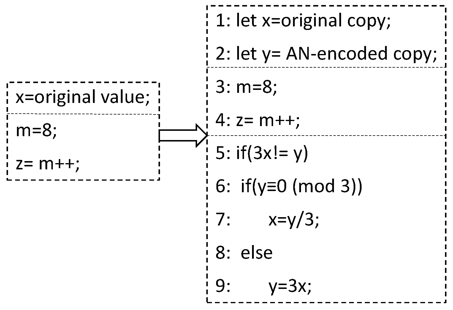
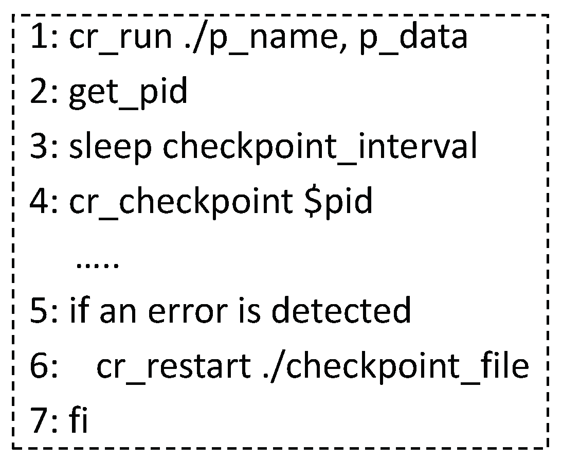
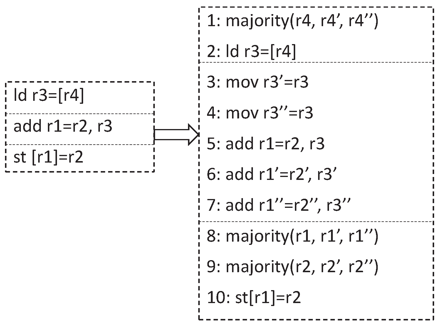
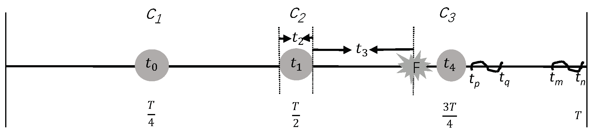
3. Preliminaries
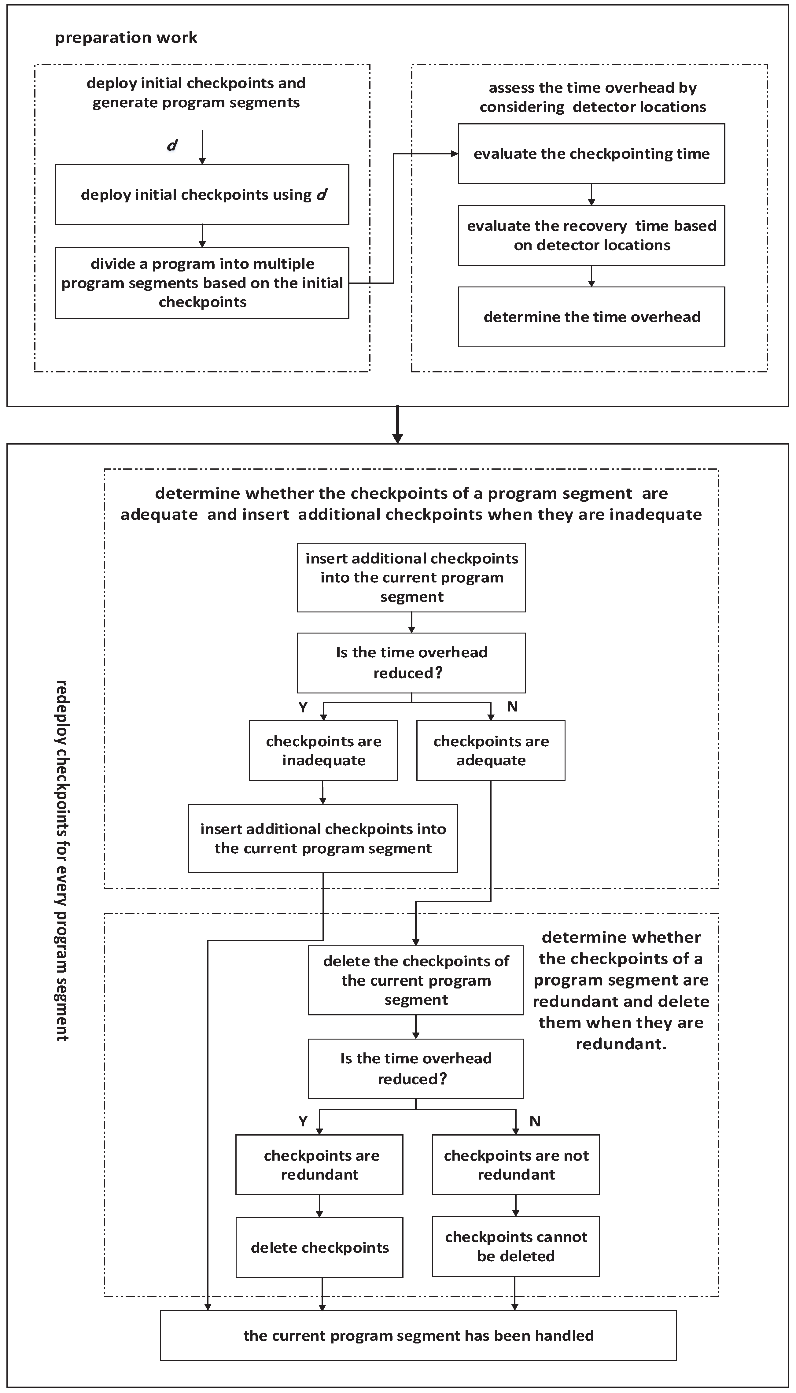
4. Overview of the DLCKPT Approach
5. The DLCKPT Approach
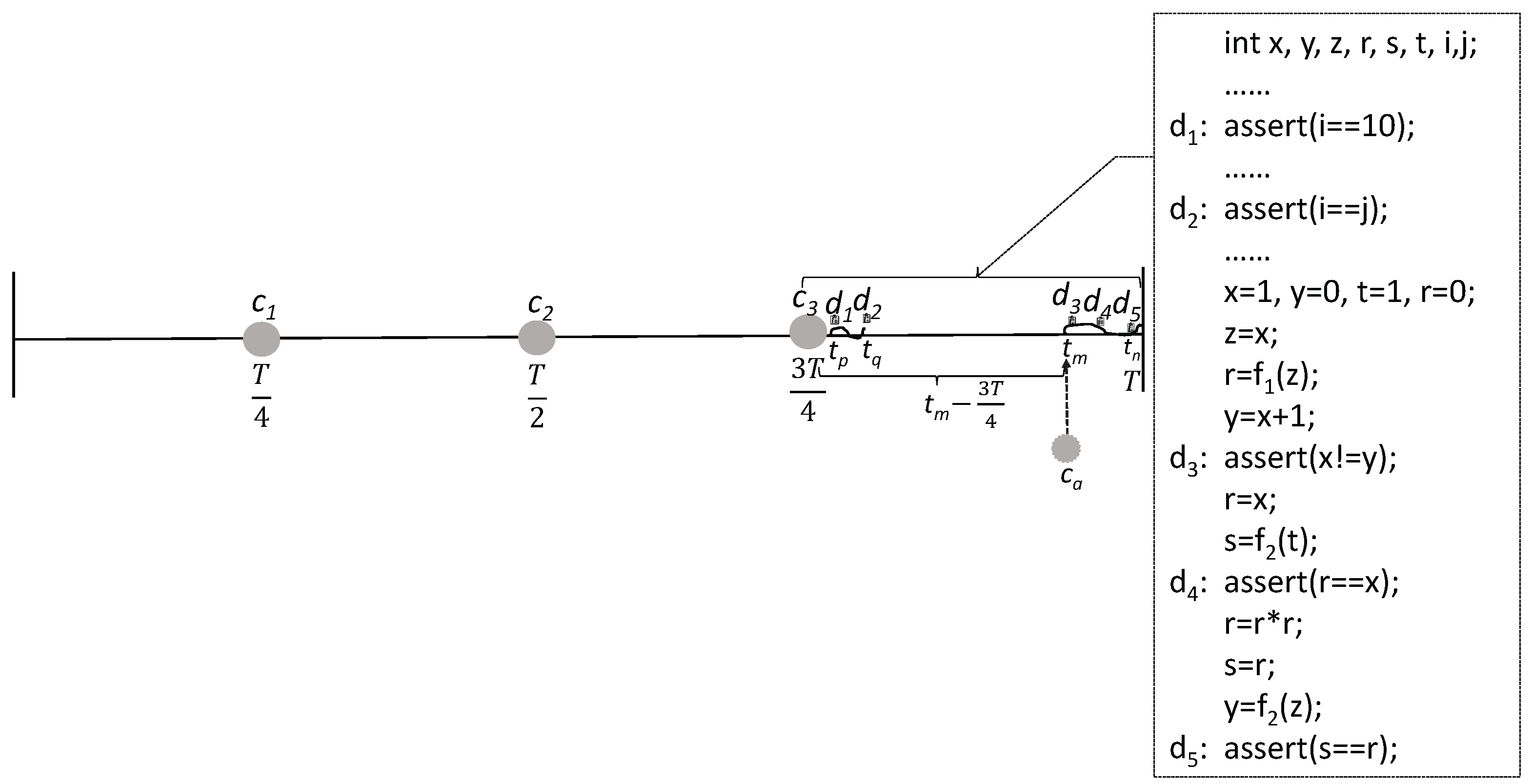
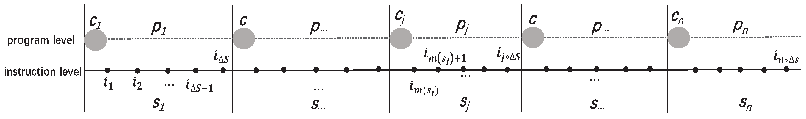
5.1. Deploy Initial Checkpoints and Generate Program Segments
5.2. The Time Overhead of a Program Segment
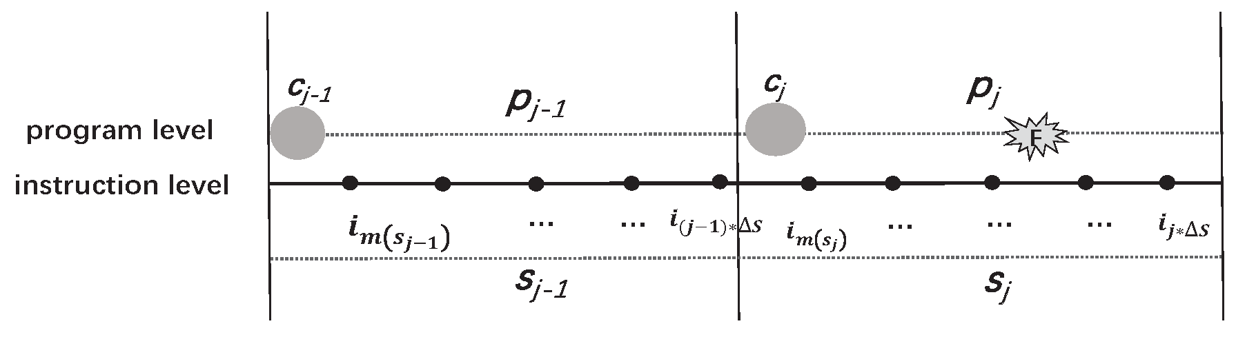
5.3. Determine the Adequacy of Checkpoints
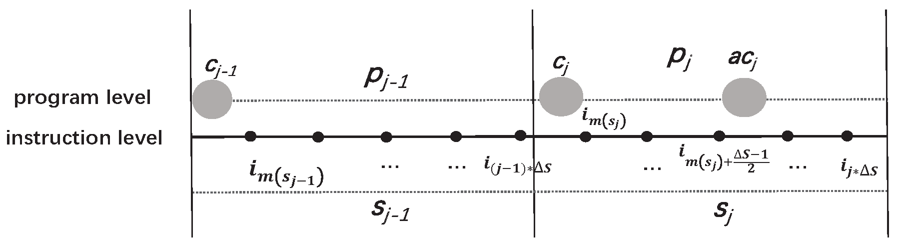
5.4. Determine the Redundancy of Checkpoints
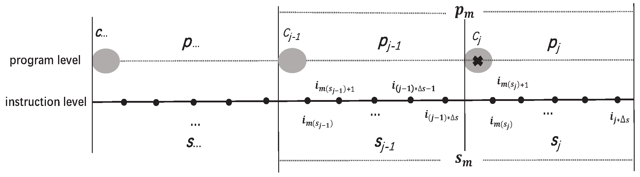
5.5. The Process of DLCKPT
| Algorithm 1 The Processes of the First Two Parts of DLCKPT |
|
| Algorithm 2 The Processes of the Last Two Parts of DLCKPT |
|
6. Experiment and Results
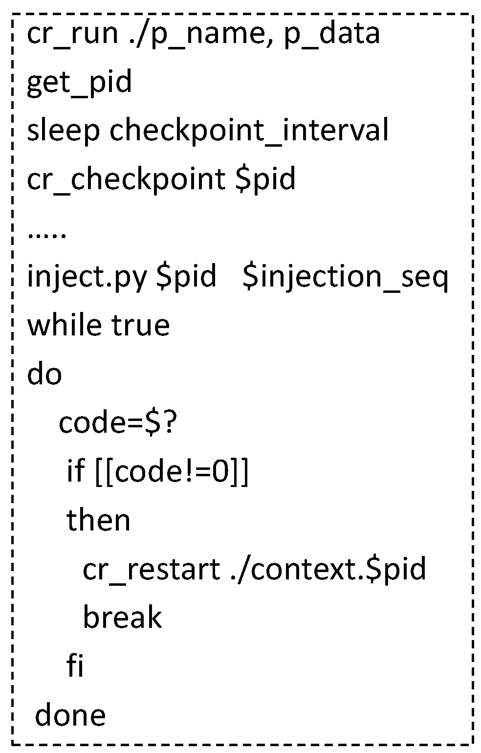
6.1. Experimental Setup
6.2. Experimental Results and Evaluation
6.2.1. The Overall Program Execution Time When a Soft Error Is Detected
6.2.2. The Overall Program Execution Time When a Soft Error Occurs
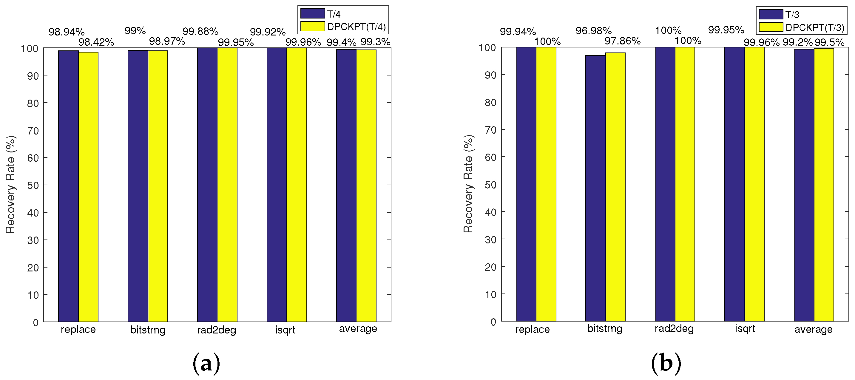
6.2.3. Recovery Rate
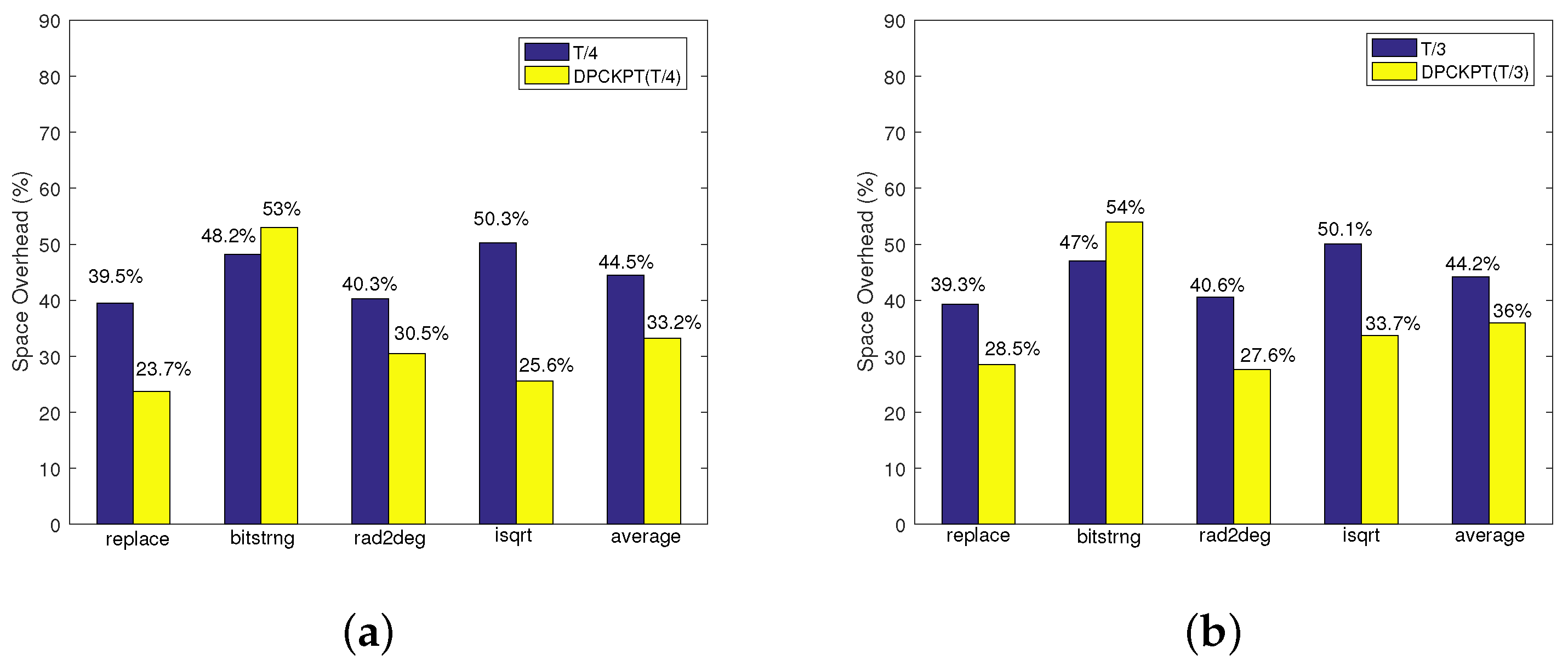
6.2.4. Space Overhead
7. Conclusions and Future Work
Author Contributions
Funding
Conflicts of Interest
References
- Gupta, N.; Shah, A.P.; Kumar, R.S.; Gupta, T.; Khan, S.; Vishvakarma, S.K. On-Chip Adaptive VDD Scaled Architecture of Reliable SRAM Cell with Improved Soft Error Tolerance. IEEE Trans. Device Mater. Reliab. 2020, 20, 694–705. [Google Scholar] [CrossRef]
- Hashimoto, M.; Liao, W. Soft Error and Its Countermeasures in Terrestrial Environment. In Proceedings of the 25th Asia and South Pacific Design Automation Conference (ASP-DAC), Beijing, China, 13–16 January 2020; pp. 617–622. [Google Scholar]
- Binder, D.; Smith, E.C.; Holman, A.B. Satellite Anomalies from Galactic Cosmic Rays. IEEE Trans. Nucl. Sci. 1975, 22, 2675–2680. [Google Scholar] [CrossRef]
- Ma, J.C.; Yu, D.Y.; Wang, Y.; Cai, Z.B.; Zhang, Q.X.; Hu, C. Detecting Silent Data Corruptions in Aerospace-Based Computing Using Program Invariants. Int. J. Aerosp. Eng. 2016, 2016, 1–10. [Google Scholar] [CrossRef]
- Tan, C.Y.; Li, Y.; Cheng, X.; Han, J.; Zeng, X.Y. General Efficient TMR for Combinational Circuit Hardening Against Soft Errors and Improved Multi-Objective Optimization Framework. IEEE Trans. Circuits Syst. 2021, 68, 3044–3057. [Google Scholar] [CrossRef]
- Kiani, V.; Reviriego, P. Improving Instruction TLB Reliability with Efficient Multi-bit Soft Error Protection. Microelectron. Reliab. 2019, 93, 29–38. [Google Scholar] [CrossRef]
- Keller, A.M.; Wirthlin, M.J. Partial TMR for Improving the Soft Error Reliability of SRAM-Based FPGA Designs. IEEE Trans. Nucl. Sci. 2021, 68, 1023–1031. [Google Scholar] [CrossRef]
- Didehban, M.; Lokam, S.R.D.; Shrivastave, A. InCheck: An In-application Recovery Scheme for Soft Errors. In Proceedings of the 54th ACM/EDAC/IEEE Design Automation Conference, Austin, TX, USA, 18–22 June 2017; pp. 1–6. [Google Scholar]
- Ma, J.C.; Duan, Z.T.; Tang, L. GATPS: An Attention-based Graph Neural Network for Predicting SDC-causing Instructions. In Proceedings of the 39th VLSI Test Symposium, San Diego, CA, USA, 25–28 April 2021; pp. 1–6. [Google Scholar]
- Yang, N.; Wang, Y.F. Radish: Enhancing Silent Data Corruption Detection for Aerospace-Based Computing. Electronics 2021, 10, 61. [Google Scholar] [CrossRef]
- Benacchio, T.; Bonaventura, L.; Altenbernd, M.; Cantwell, C.D.; Düben, P.D.; Gillard, M.; Giraud, L.; Göddeke, D.; Raffin, E.; Teranishi, K.; et al. Resilience and Fault Tolerance in High-Performance Computing for Numerical Weather and Climate Prediction. Int. J. High Perform. Comput. Appl. 2021, 35, 285–311. [Google Scholar] [CrossRef]
- Didehban, M.; Shrivastava, A. A Compiler Technique for Processor-Wide Protection From Soft Errors in Multithreaded Environments. IEEE Trans. Reliab. 2018, 67, 249–263. [Google Scholar] [CrossRef]
- Reis, G.A.; Chang, J.; August, D.I. Automatic Instruction-Level Software-Only Recovery. IEEE Micro 2007, 67, 36–47. [Google Scholar] [CrossRef]
- Guo, Y.M.; Wu, H.; Chai, W.X.; Ma, J.Z.; Zhou, G.C. Integrity Checking based Soft Error Recovery Method for DSP. In Proceedings of the Prognostics and System Health Management Conference, Chengdu, China, 19–21 October 2016; pp. 1–4. [Google Scholar]
- Yang, N.; Wang, X.; Wang, Y.; Zhai, Q. Dependent and Heterogeneous Process Migration Based on Checkpoints. In Proceedings of the IEEE International Conference on Parallel and Distributed Processing with Applications, Big Data and Cloud Computing, Exeter, UK, 17–19 December 2020; pp. 84–92. [Google Scholar]
- Restrepo-Calle, F.; Martĺnez-Álvarez, A.; Cuenca-Asensi, S.; Jimeno-Morenilla, A. Selective SWIFT-R: A Flexible Software-Based Technique for Soft Error Mitigation in Low-Cost Embedded Systems. J. Electron. Test. 2013, 29, 825–838. [Google Scholar] [CrossRef]
- Didehban, M.; Shrivastava, A.; Lokam, S.R.D. NEMESIS: A Software Approach for Computing in Present of Soft Errors. In Proceedings of the IEEE International Conference on Computer-Aided Design, Irvine, CA, USA, 13–16 November 2017; pp. 297–304. [Google Scholar]
- Amrizal, M.A.; Uno, A.; Sato, N.Y.; Takizawa, H.; Kobayashi, H. Energy-Performance Modeling of Speculative Checkpointing for Exascale Systems. IEICE Trans. Inf. Syst. 2017, 12, 2749–2760. [Google Scholar] [CrossRef]
- Quezada-Sarmiento, P.A.; Elorriaga, J.A.; Arruarte, A.; Jumbo-Flores, L.A. Used of Web Scraping on Knowledge Representation Model for Bodies of Knowledge as a Tool to Development Curriculum. In Trends and Applications in Information Systems and Techinologies; Springer: Berlin, Germany, 2021; Volume 2, pp. 611–620. [Google Scholar]
- Ma, J.C.; Duan, Z.T.; Tang, L. Deep Soft Error Propagation Modeling Using Graph Attention Network. J. Electron. Test. 2022, 38, 303–319. [Google Scholar] [CrossRef]
- Sharanyan, S.; Kumar, A. An optimized Checkpointing Based Learning Algorithm for Single Event Upsets. In Proceedings of the IEEE International Conference on Annual Computer Software and Applications, Seoul, Republic of Korea, 19–23 July 2013; pp. 395–400. [Google Scholar]
- Subasi, O.; Krishnamoorthy, S. On the Theory of Speculative Checkpointing: Time and Energy Considerations. In Proceedings of the ACM International Conference on Computing Frontiers, Ischia, Italy, 8–10 May 2018; pp. 165–172. [Google Scholar]
- Sangchoolie, B.; Pattabiraman, K.; Karlsson, J. An Empirical Study of the Impact of Single and Multiple Bit-Flip Errors in Programs. IEEE Trans. Dependable Secur. Comput. 2020, 2020, 1–18. [Google Scholar] [CrossRef]
- Yang, N.; Wang, Y. Predicting the Silent Data Corruption Vulnerability of Instructions in Programs. In Proceedings of the IEEE International Conference on Parallel and Distributed Systems, Tianjin, China, 4–6 December 2019; pp. 862–869. [Google Scholar]
- Li, G.P.; Pattabiraman, K.; Hari, S.K.S.; Sullivan, M.; Tsai, T. Modeling Soft-Error Propagation in Programs. In Proceedings of the IEEE International Conference on Dependable Systems and Networks, Luxembourg, 25–28 June 2018; pp. 27–38. [Google Scholar]
- Ma, J.C.; Wang, Y. Characterization of Stack Behavior under Soft Errors. In Proceedings of the Design, Automation & Test in Europe Conference & Exhibition, Lausanne, Switzerland, 27–31 March 2017; pp. 1534–1539. [Google Scholar]


| Name | Meaning |
|---|---|
| Checkpointing time | The time required to preserve a program’s running state. |
| Recovery time of a historical state | The time required to restore the data of the latest checkpoint. |
| Recovery time of a current state | The time required to execute a program from the latest checkpoint to the place where an error is reported by a detector. |
| Recovery time | The time required to recover the historical state and current state. |
| Fault tolerance time | The checkpointing time and recovery time. |
| Overall program execution time | The original program execution time and fault tolerance time. |
| Programs | T/4 | T/3 |
|---|---|---|
| replace | 22.1% | 14.1% |
| bitstrng | 4% | 8% |
| rad2deg | 10% | 10% |
| isqrt | 22.3% | 13.5% |
| average | 15% | 11.4% |
| Programs | T/4 | T/3 |
|---|---|---|
| replace | 25.6% | 15.3% |
| bitstrng | 3% | 2% |
| rad2deg | 11% | 12% |
| isqrt | 23.2% | 14.5% |
| average | 16% | 11% |
Disclaimer/Publisher’s Note: The statements, opinions and data contained in all publications are solely those of the individual author(s) and contributor(s) and not of MDPI and/or the editor(s). MDPI and/or the editor(s) disclaim responsibility for any injury to people or property resulting from any ideas, methods, instructions or products referred to in the content. |
© 2023 by the authors. Licensee MDPI, Basel, Switzerland. This article is an open access article distributed under the terms and conditions of the Creative Commons Attribution (CC BY) license (https://creativecommons.org/licenses/by/4.0/).
Share and Cite
Yang, N.; Wang, Y. A Checkpointing Recovery Approach for Soft Errors Based on Detector Locations. Electronics 2023, 12, 805. https://doi.org/10.3390/electronics12040805
Yang N, Wang Y. A Checkpointing Recovery Approach for Soft Errors Based on Detector Locations. Electronics. 2023; 12(4):805. https://doi.org/10.3390/electronics12040805
Chicago/Turabian StyleYang, Na, and Yun Wang. 2023. "A Checkpointing Recovery Approach for Soft Errors Based on Detector Locations" Electronics 12, no. 4: 805. https://doi.org/10.3390/electronics12040805