Mitigating Catastrophic Forgetting with Complementary Layered Learning

Abstract

Catastrophic forgetting is a stability–plasticity imbalance that causes a machine learner to lose previously gained knowledge that is critical for performing a task. The imbalance occurs in transfer learning, negatively affecting the learner’s performance, particularly in neural networks and layered learning. This work proposes a complementary learning technique that introduces long- and short-term memory to layered learning to reduce the negative effects of catastrophic forgetting. In particular, this work proposes the dual memory system in the non-neural network approaches of evolutionary computation and Q-learning instances of layered learning because these techniques are used to develop decision-making capabilities for physical robots. Experiments evaluate the new learning augmentation in a multi-agent system simulation, where autonomous unmanned aerial vehicles learn to collaborate and maneuver to survey an area effectively. Through these direct-policy and value-based learning experiments, the proposed complementary layered learning is demonstrated to significantly improve task performance over standard layered learning, successfully balancing stability and plasticity.

1. Introduction

Layered learning is a machine learning paradigm that develops autonomous computerized agents through task decomposition, incremental learning, and transfer learning. The paradigm excels at solving complex problems with large search spaces by decomposing a task into a series of subproblems (subtasks) and maximizing its decision-making policy one subtask at a time. By containing each subtask within its own layer, the policy is incrementally shaped toward the solution with a smaller search space to navigate through. The paradigm has gained popularity due to its efficient shaping of the robotic training agents to learn to solve a problem through task decomposition, hierarchical sequencing of those subtasks, and transfer learning that builds competency incrementally.

Unfortunately, the incremental learning methodology and transfer of knowledge from one subtask to another can negatively and drastically change the layer learner’s ability to retain new and previously obtained knowledge through catastrophic forgetting. Catastrophic forgetting results in a learner’s complete loss of critical knowledge (forgetting) that is needed to perform a subtask. This work demonstrates that layered learning is susceptible to catastrophic forgetting and examines the root cause: stability–plasticity imbalance.

Maintaining stability–plasticity imbalance is a dilemma faced by machine learning approaches (i.e., robot shaping, transfer learning, and incremental learning). The dilemma challenges learners to find a balance between retaining important information used to perform previously learned behaviors while learning to solve new problems [1]. When the learner favors plasticity, the imbalance often results in the learner’s loss of proficiency in learned, older tasks in favor of new, incoming knowledge. Often, these newer tasks have higher priority than older tasks because of changes in the agent’s environment, state, and other agents in the learning scenario. On the other hand, when the agent favors stability, the imbalance prioritizes older knowledge, struggles to adapt to changes, and underperforms on newer tasks in a reinforcement environment.

Recently, the stability–plasticity imbalance has been demonstrated to occur in layered learning with direct-policy searches [2]. These demonstrations have shown that layered learning agents can experience significant decreases in previously learned task performances, wasted learning time, and increases in training time, and agent decision-making policies are unable to regain achieved proficiencies because previous knowledge is forgotten forever.

To further understand why critical knowledge can be forgotten in implementations of the paradigm, this work extends the study by first establishing that layered learning can also experience a heavy imbalance when the underlying algorithm is a value-based search. With demonstrations of catastrophic forgetting in non-neural network direct-policy and value-based searches, we provide evidence that the paradigm is hindered from optimal performance. We focus on non-neural network approaches because real, physical robots are being deployed with other transfer learning approaches, such as evolutionary computation and Q-learning, which are traditionally faster to design, more efficient to compute, and easier to analyze and explain, due to their simpler architectures, compared with deep learning models. Therefore, to remedy these negative impacts on these machine learning approaches, this work introduces a new method to mitigate catastrophic forgetting and establish a stability–plasticity balance among layered learning agents. In particular, this work introduces a complementary form of learning that augments standard layered learning with long- and short-term memory. This complementary layered learning approach determines which knowledge is valuable for the overall task as the agent transfers knowledge from one subtask to another.

In this paper, layered learning is described, layered learning’s imbalance is reviewed, the new complementary layered learning technique is defined, and experiment results are presented, demonstrating that equilibrium is possible within the learning paradigm.

2. Background

Layered learning has gained popularity as a method for generating intelligent agents, as implementations of the paradigm have led to success in robot competitions [3,4]. Centered on transfer learning and robot shaping, layered learning decomposes a task with a large search space (both action- and observation-spaces) into smaller subtasks. The learning agent then learns each subtask sequentially, adapting its decision-making capability (policy) until it obtains proficiency with each subtask. To drive this incremental learning, the agent iterates over a set of layers, where each layer contains a subtask to optimize on, a learning algorithm (evolutionary computation, Q-learning, deep learning, etc.), a training environment, a training scenario, a halting condition, and the agent’s policy to modify and optimize on that layer’s subtask. The agent continuously trains in a layer until that layer has satisfied its halting condition. The halting condition can be defined as the situation when the agent reaches a specific proficiency or when a predetermined number of learning iterations elapses. Once a layer is complete, the policy of that layer is inputted into the next layer, where it optimizes the policy on a new subtask. The agent should have a level of proficiency in the overall task when it has exhausted all of its layers. Traditionally, the subtask of the last layer is the overall, complex task and all subsequent layers have steered the agent toward a policy that assembles all of the previous layers’ knowledge. The paradigm was designed to decompose the overall task’s search space into a series of smaller spaces.

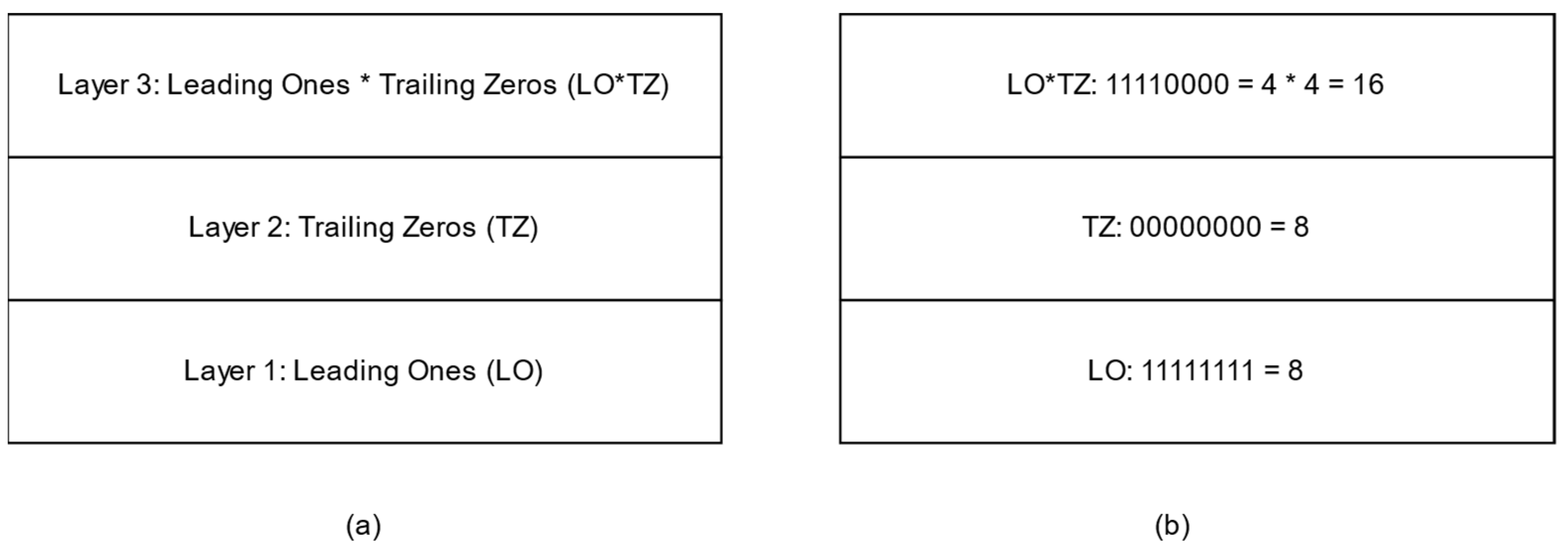
To illustrate layered learning and its policy transformation, let us consider the Leading Ones * Trailing Zeros (LO*TZ) problem. The goal in LO*TZ is to generate a bitstring that maximizes the product of the number of ones in the prefix (leading ones) and the number of zeros in the suffix (trailing zeros). For optimal bitstring generation, the agent flips its bits between one and zero to find the bitstring that maximizes its performance criteria. For example, in a bitstring of 8, the ideal LO*TZ solution will have the string start with four ones in the prefix, followed by four zeros in the suffix, resulting in a performance score of 4 × 4 = 16. In this example, LO*TZ is decomposed into three layers: LO, TZ, and LO*TZ. Figure 1 displays a layered learning configuration for the LO*TZ problem. Layer one evaluates a bitstring on the number of leading ones (LO), which is the number of continuous ones in the bitstring’s prefix. This layer’s maximum score is 8, representing a bitstring that is made up entirely of ones and reflects a maximum prefix of leading ones. The second layer evaluates the performance of trailing zeros (TZ). Here, the bitstring’s optimal performance would result in eight uninterrupted bits in the suffix. The final layer, layer three, aggregates the first two layers and evaluates the bitstring on the LO*TZ problem, multiplying the all-ones prefix and all-zeros suffix. In this example, the first two layers serve as objectives of the overall problem’s goal of LO*TZ. Additionally, the bitstring abstractly represents an agent’s policy, whereas the bit index and value can represent the agent’s state- and action-space.

Beyond theory, layered learning successfully reduces the search space into more navigable problems in implemented instances of deployed machine learning. In fact, compared to traditional single-optimization approaches, layered learning has outperformed monolithic learning in various domains [3,4,5,6,7,8,9,10,11,12,13,14]. Hsu and Gustafson [5,6,7] demonstrated the increased performance layered learning brings to simulated soccer players, while Cherubini [8], Fidelman and Stone [9], and Leottau [10] extended the work to physical robots and observed performance improvements as well. Further, Jackson and Gibbons [11] and Mondesire and Wiegand [12] showed that Boolean logic problems also showed performance improvements and reduction in training time with layered learning, while Mondesire and Wiegand [13] demonstrated that layered learning also reduces learning time among non-playable characters in a predator–prey environment. These works accredit layered learning’s search space reduction and incremental learning as the reason for performance improvement.

2.1. Catastrophic Forgetting in Layered Learning with Boolean Logic Problems

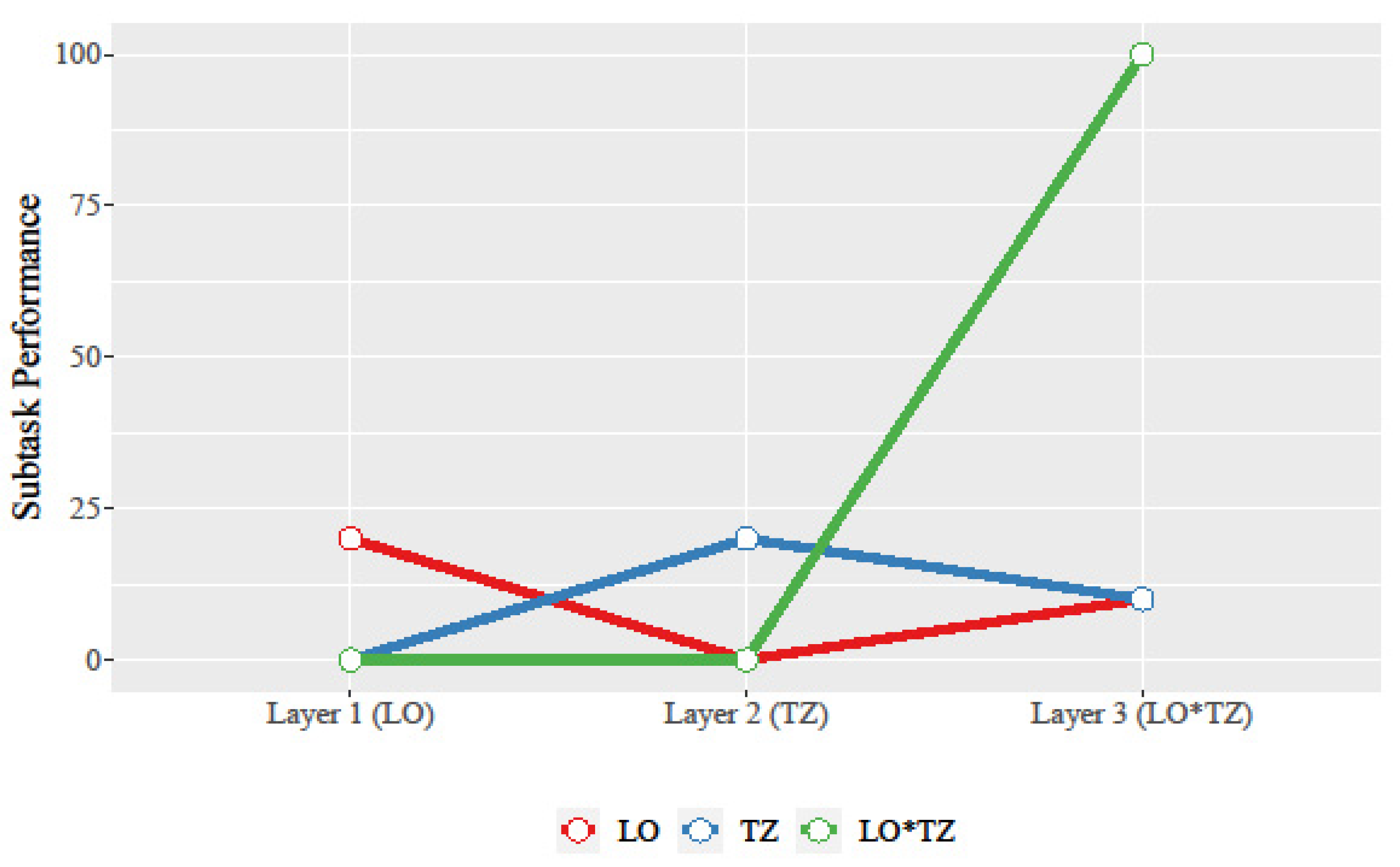
Several layered learning studies observed decreases in the overall task and individual subtask performance as the learner transitioned to new layers and their subtasks. To study and demonstrate the loss in proficiency, a preliminary study examined layered learning’s knowledge loss using the LO*TZ program and layer configuration described earlier [12]. In that work, knowledge gained from previously optimized subtasks was driven out when new subtasks were introduced. Specifically, when the agent optimized its policy on the TZ subtasks, the performance of the previously trained LO subtasks plummeted. In an extended example of the LO*TZ problem, Figure 2 displays how subtask performance changed as each layer elapsed with a bitstring of 20 bits. In Layer 1, the agent achieved optimal LO performance with a maximum LO score of 20, while TZ’s score was zero because the bitstring contained all ones, similar to Figure 1b’s LO bitstring. At the end of Layer 2, the TZ optimization resulted in a bitstring of all zeros, for a TZ maximum score of 20 and an LO minimum score of zero. Layer 2 drove out all of the LO policy knowledge to favor the TZ function. In addition, LO*TZ performance is zero at the end of both layers because one subtask has a performance score of zero, nullifying the overall task performance. The third layer trained the policy on the LO*TZ aggregate and overall task, which also led to the previous subtask performances (both LO and TZ) decreasing their highest observed score in order to maximize the LO*TZ task performance; this achieved overall score of 100 is calculated from a score of 10 from LO’s all-ones 10-bit prefix multiplied by the 10 score from the 10 zero-bit suffix.

This work used the LO*TZ problem to deliberately exacerbate forgetting and to specifically study the effects of a policy when the overall goal comprises an aggregation of competing subtasks. Importantly, the work demonstrated, in a simple and explainable scenario, that previously learned knowledge could be completely driven out of an agent in the incremental and transfer learning paradigm.

2.2. Catastrophic Forgetting in Layered Learning within Multi-Agent Systems

To extend the imbalance demonstration to a real-world scenario, the authors of this paper studied layered learning in a direct-policy search for a multi-agent system [2]. In that study, multiple independent decision-making agents learned to conduct an aerial surveying task, where the team had to traverse the entire area of a large territory. The agents represented a team of collaborating quadcopter unmanned aerial vehicles (UAVs). In this study, each UAV learned to take off, land, move to waypoints and coordinates, refuel (charge its batteries), and transmit coordinates to teammates. Without communication, coordination, and efficient planning, the UAV team could not survey the entire 50 × 50 grid map area under the team’s time constraints (2000 timesteps, where each agent could move one cell per timestep). This UAV surveying problem was derived from other search-and-rescue and drone navigation problems found in the literature and in real-world scenarios [15,16]. 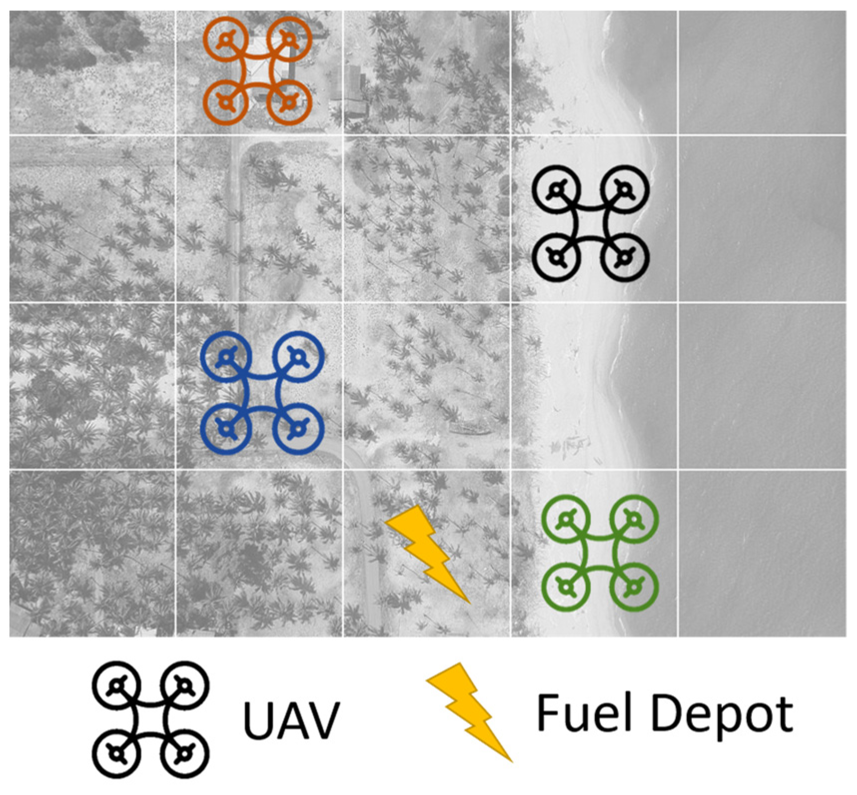Figure 3 is a visual representation of the UAV simulator, displaying a portion of the grid map. In the figure, the four UAVs are actively surveying the area and have a choice to land at a fuel depot to recharge their batteries.

To facilitate the UAVs’ learning of the overall surveying task, each agent was given three layers: (1) refuel, (2) take-off and survey, and (3) the UAV surveying problem. Layer 1’s subtask was to learn to refuel when the UAV’s battery was low. Individual UAVs were awarded a maximum reward if they could land at a depot and refuel their battery. Layer 2 optimized the agents on the take-off and survey subtask by evaluating the UAVs’ ability to transition from a grounded state and move around the map. The reward was the amount of unique grid map locations the UAV reached. Layer 3 contained the overall task of the UAV surveying problem. Layer 3 was the aggregate of the first two layers, because the UAVs must learn to move to a refueling depot, execute the refueling action, take-off and survey, communicate traversed coordinates, and coordinate with teammates to minimize duplication and wasted time. In this final layer, the UAVs received a shared reward for the number of unique coordinates the UAV team traversed.

In the preliminary UAV study [2], all of the agents learned the surveying task with a direct-policy search method implemented with a (1+1) Evolutionary Algorithm, also known as a (1+1) EA [17,18]. The (1+1) EA is a simplified version of a traditional evolutionary algorithm, where the population size is reduced to just one chromosome and only the mutation operator is used to modify the policy. With this approach, the policy was represented by a one-dimensional chromosome array of state-to-action mappings (pairs) of each agent. Each state corresponded with an action to take. The possible actions included “take-off”, “navigate towards next unvisited coordinate”, “land”, “NOP” (remain idle), “move towards the closest fuel depot”, “refuel”, and “transmit coordinates”. All movement actions take the UAV to the most efficient route to its destination. Unique UAV states combined agent statuses of “is my fuel level low”, “am I grounded”, “am I at a fuel depot”, “is my fuel level above 90% full”, and states determining whether a UAV’s communication buffer size contains 1, 5, 10, or 20 coordinates to transmit.

This paper extends the earlier study by examining the imbalance when the underlying machine learning algorithm is a value-based search. In this extended experiment, all layers deploy Q-learning to discover the optimal UAV agent policy. Specifically, Q-learning modifies the policy’s q-table for decision-making instead of the (1+1) EA’s single chromosome policy for each agent, where the q-value is updated after an action is performed and a reward is returned [19]. Immediate rewards are dispersed by the simulator to individual UAVs but all invalid actions yield rewards of zero. The same states, actions, rewards, and experiment conditions were used in the Q-learning implementations as the (1+1) EA, including training time, initial scenario conditions, and the number of runs. For instance, each layer had a limitation of 10,000 episodes, so the total training time was 30,000 episodes per experiment run. Further, each machine learning approach’s experiments were repeated for 100 runs and started with the same initial random seed. Additional parameters included the optimized Q-learner’s learning rate (α = 0.2) and discount factor (γ = 0.1). Finally, a uniform epsilon-decreasing strategy was used to select the highest q-value action at a proportion of 1-εꢀꢀ of the elapsed time; this incorporated exploration at the beginning of a layer’s learning phase and exploitation toward the end.

The UAV problem and its action space of the experiment were deliberately designed to study a heavily-plasticity scenario and a problem derived from real-world robotics problems that need improved solutions through advancements in machine learning. Additionally, the experiments were purposefully designed to exhibit that as the evaluation criteria for the agents’ transition, the pairs of each agent’s policy experienced significant modifications to reflect the new function to optimize on. Consequently, subtask and task performance were degraded during these transitions and learning effort was lost when a policy attempted to regain its forgotten subtask proficiency.

The imbalance was witnessed in the (1+1) EA and Q-learning experiments, as demonstrated in how the policies were modified to favor newer subtasks and how their composition changed altered proficiencies in older, learned subtasks. For example, [2] reported that after the refueling layer transitioned to take-off and survey, the refueling performance decreased by 58%; a comparative decline was also observed when transitioning from take-off and survey to the overall UAV survey layer. The pattern continued with Q-learning: once the policies optimized on Layer 1’s refueling capability with a 100% optimality score, refueling proficiency was lost in Layer 2 with a 0% performance score.

Table 1. The average performance of each subtask per layer completion for Q-learning.

Algorithm	Layer	Refuel	Take-Off and Survey	UAV Surveying Task
Q-learning	1	1.0	0.048	0.046
	2	0.0	0.824	0.13
	3	0.753	0.728	0.369

captures the average subtask performance of each learner after each layer for Q-learning while the work in [2] captured the results of the (1+1) EA.;

Table 2. The standard deviation for each subtask per layer completion for Q-learning.

Algorithm	Layer	Refuel	Take-Off and Survey	UAV Surveying Task
Q-learning	1	0.0	0.061	0.13
	2	0.0	0.027	0.004
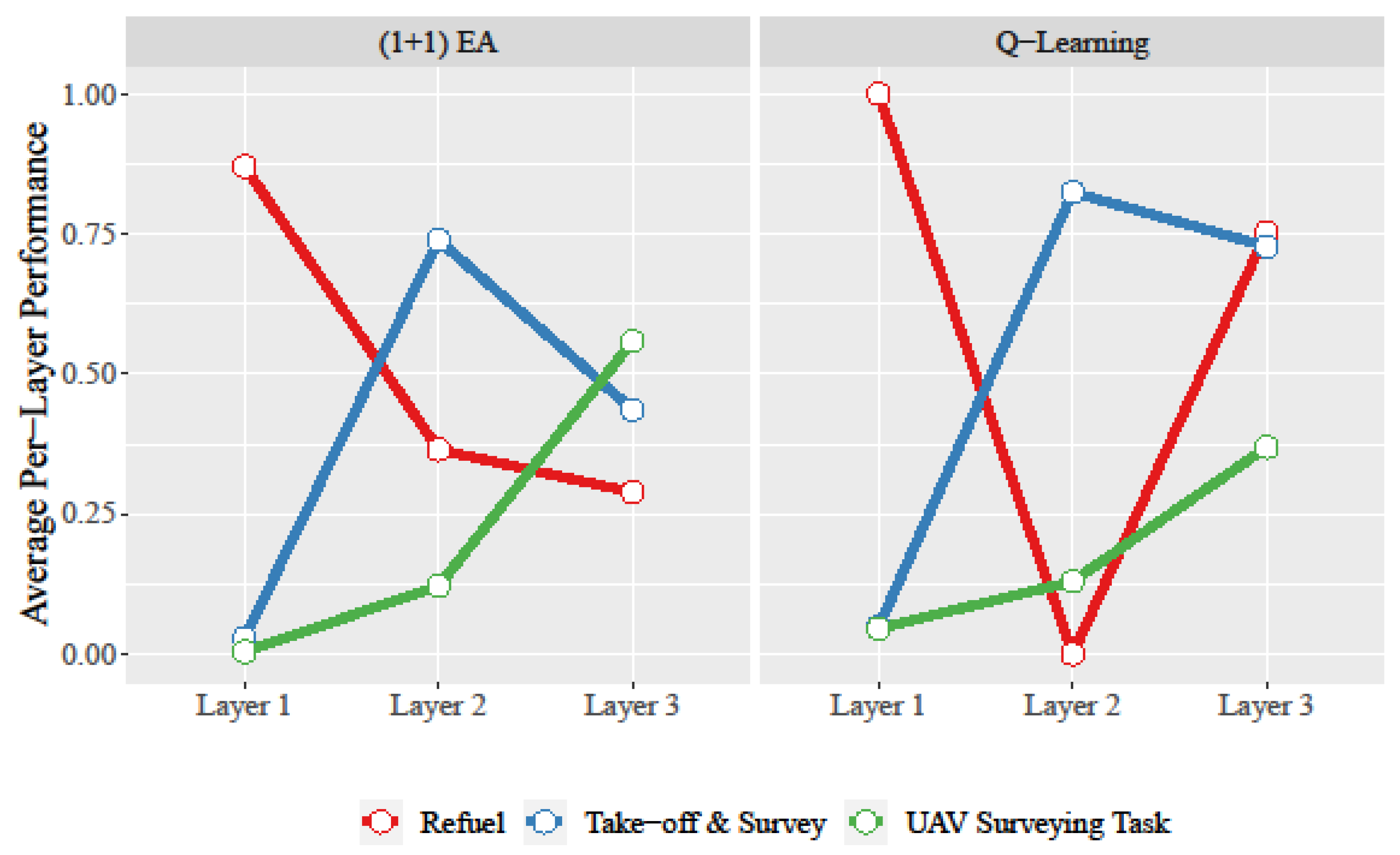
	3	0.006	0.024	0.083

contains the standard deviation of the layer transitions. The (1+1) EA decreased the performance of the subtask when the learner transitioned to the next layer and optimized on another subtask. Therefore, the policy changes between Layers 1 and 2 resulted in UAVs failing to perform all measurable aspects of the refueling subtask. The “take-off and survey” subtask also experienced significant proficiency loss, from 82% to 73%, from the final transition from Layer 2 to Layer 3. This observation is depicted in Figure 4, showing how the refuel performance plummeted from Layers 1 to 2, and the take-off and survey performance decreased between Layers 2 and 3.

These demonstration experiments corroborated the layered learning Boolean logic conclusions reported in [12] by observing that past knowledge was being driven out of layered learning policies as the evaluation function changed. For example, the (1+1) EA for this work’s UAV surveying task, as shown in Figure 4, followed a similar pattern as that experienced with the LO*TZ problem in Figure 2; both sets of experiments observed that as the policy transitioned to a new layer and new evaluation criteria, layer overlapping (where layers can affect parts of a policy shared by another layer) and conflicting objectives resulted in a previously learned skill to significantly decrease in performance. These works provide evidence that supports why it is necessary to develop new techniques to mitigate the imbalance that heavily favors plasticity. Advancements in the learning paradigm could preserve important knowledge gained in earlier layers to speed up the overall task training of the policy and potentially improve the overall effectiveness of the agent system.

2.3. Catastrophic Forgetting in Other Machine Learning Approaches

In machine learning, this phenomenon of losing previously learned knowledge is not new; other transfer learning methods and paradigms are also susceptible. Jin and Sendhoff [20] claimed that balancing stability and plasticity is a challenge all learners should consider. As subsequently identified by McCloskey and Cohen [1], many machine learning techniques have analyzed the dilemma and have addressed its occurrence. In fact, catastrophic forgetting [20] was first termed in machine learning to address the driving out of critical knowledge in artificial neural networks and later used to describe when skill proficiency is completely lost from an agent’s trained policy, model, or network [21,22]. In neural networks, catastrophic forgetting occurs when the network is retrained on new data or tasks, causing the weights and biases to be altered so much that the network can no longer perform as well on previously trained data or tasks [23].

Complementary learning systems are the prominent solution to balance stability and plasticity in neural networks. These approaches introduce the concept of dual memory to the learning process, often employing a variant of short- and long-term memory [24]. In brief, the neural network transfers information between the two memory regions, often based on how frequently the information has been accessed. Some examples of two-phased learning systems enhance recurrent neural networks (RNN) [21,25], including pseudo-recurrent networks [22], pseudorehearsal [23], and hippocampus–neocortical-based Hopfield networks and Hebbian learning [26]. The most widespread solutions to balancing older and newer network states include long short-term memory (LSTM) [27] and the gated recurrent unit (GRU) [28,29,30,31,32,33]. LSTMs extend the capability of RNNs to possess long- and short-term memory through their feedback input into hidden neurons. With an LSTM, RNNs extend their short-term memory capacity by retaining information acquired during long sequences of timestep changes to a network from a learning episode. An LSTM unit can be composed of a cell, an input gate, an output gate, and a forget gate that retains knowledge, controls the rate of change, and determines which updates are permitted to progress in and out of the cell [27]. Fortunately, significant attention has been given to overcoming catastrophic forgetting in neural networks, due to the popularity of deep learning and applications in the past two decades.

3. Materials and Methods

To combat catastrophic forgetting in layered learning, this work proposes a complementary augmentation to the learning paradigm, called complementary layered learning (CLL). The new enhancement is inspired by other complementary learning systems introduced in neural networks to mitigate forgetting’s negative effects. Like other complementary systems, CLL has dual memory storage regions that are introduced to retain previously learned beneficial knowledge (state–action pairs) that could have been prematurely or inadvertently removed from the policy. In this scheme, the agent has a working memory to make decisions with and a long-term memory that seeds the working memory with new knowledge (state–action pairs) or is a staging memory before knowledge is completely removed from the agent.

In the CLL process, every state–action pair in the working memory is copied into long-term memory at the conclusion of a layer. The terminal layer modifies its policy by reintroducing pairs from the long-term memory or generating new pairs, based on a user-defined long-term memory probability parameter. The approach has similarities to Trust Region Policy Optimization (TRPO) [34] and Proximal Policy Optimization (PPO) [35], which have made recent advancements in reinforcement learning with deep learning in DeepMind’s AlphaStar, AlphaGo, and AlphaFold [36,37].

Because CLL is designed to support direct-policy and value-based searches, the augmentation of the paradigm is robust. In direct-policy search, pair updates are made at a fixed probability of selecting from the long-term memory. During an update, the policy pair is updated to be a random pair from the long-term memory that matches a pair’s state. A random state-matching pair from the long-term memory is chosen because multiple pairs that match the policy pair’s state may exist. 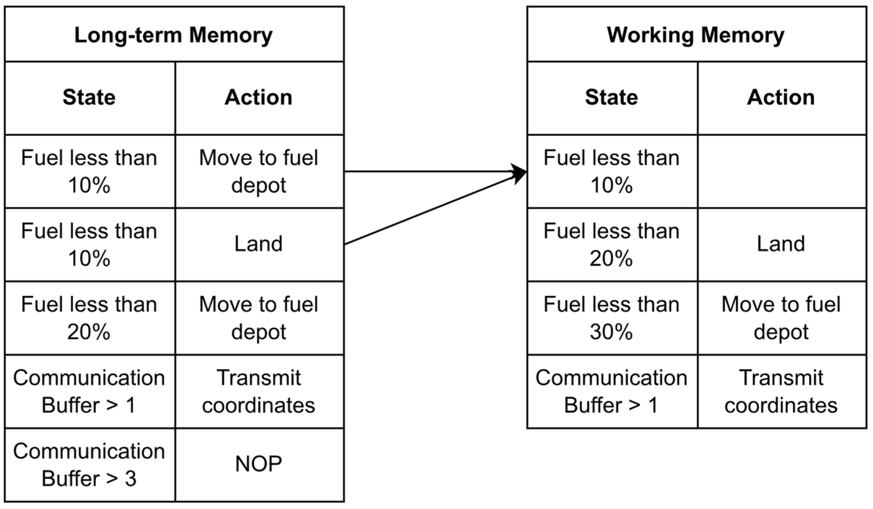Figure 5 displays a simplified policy and the reintroduction of a pair from long-term to working memory in the UAV surveying problem. In this example, the policy is updating its “Fuel less than 10%” state with one of the state-matching pairs in the long-term memory; in this case, either the “Move to fuel depot” or “Land” action will be brought into the policy. With this method, if a policy does not select a pair from long-term memory (because a pair with a matching state does not exist or because the random roll was outside of the long-term memory probability parameter), then a random action from the action space is selected and placed in working memory. Reintroducing pairs from long-term memory into working memory allows the learner to exploit past successes without needing to completely relearn knowledge of older subtasks. Additionally, long-term memory allows knowledge to remain accessible to the learner, even if the pair was removed from working knowledge many training episodes prior. As an alternative to long-term memory’s exploitation, random action selections introduce exploration in the learner’s search for a better-performing policy. The complementary learning system and the long-term memory probability parameter give the system’s designer the ability to explicitly control the stability–plasticity balance of the learning process.

The experiments evaluated CLL’s ability to perform the same UAV survey problem as [2] and, as described earlier in this paper, for the (1+1) EA and Q-learning. In this evaluation, both learning algorithms were augmented with the complementary memories of CLL and matched all of the same parameters as the aforementioned studies, including task decomposition (refuel, take-off and survey, and the UAV survey task), state space, action space, training times (10,000 episodes per layer), evaluation functions, timesteps per episode, and 100 runs per learning algorithm.

3.1. Complementary Layered Learning with a (1+1) EA

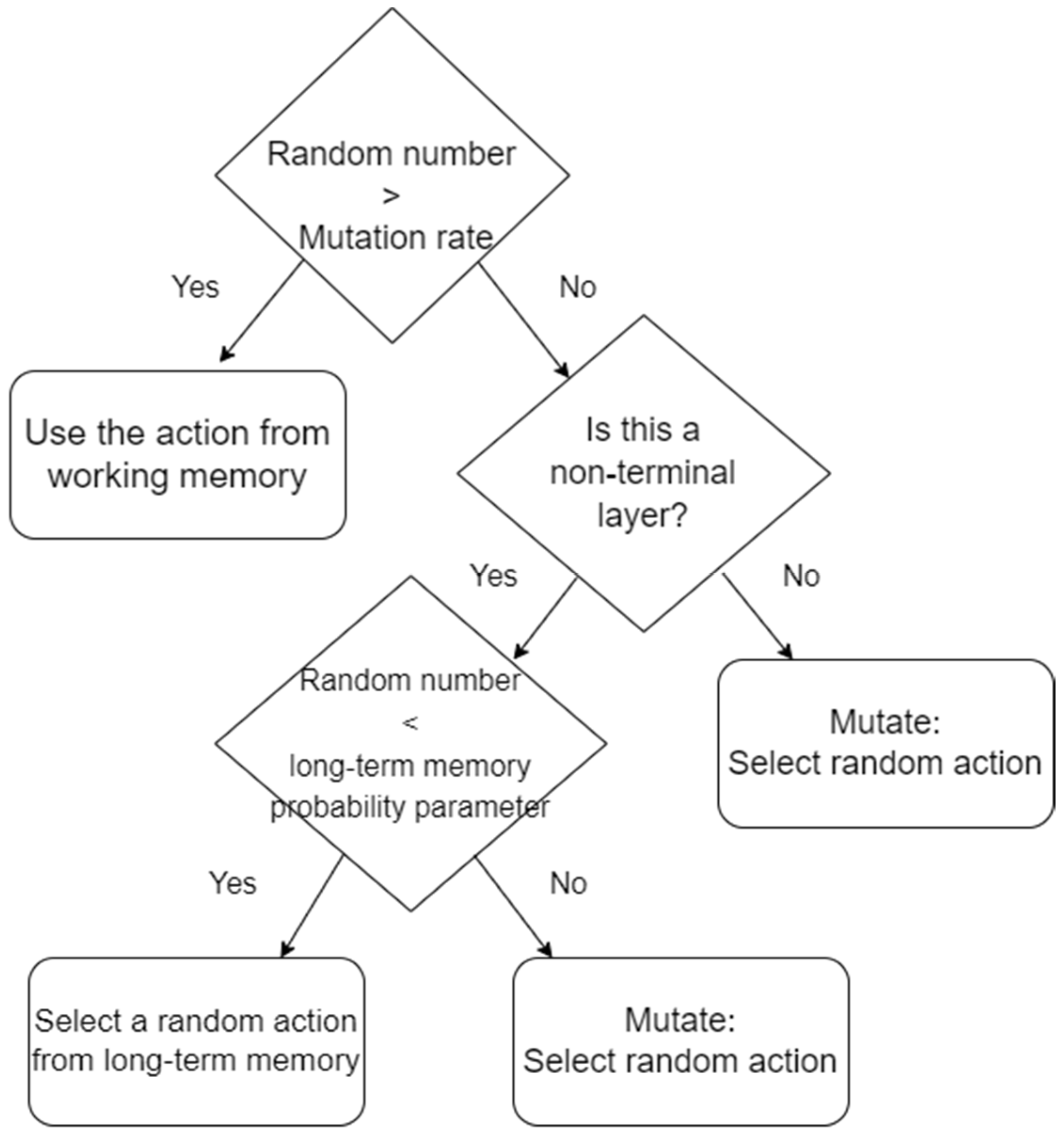
A hash map is used by complementary layered learning as the working memory in the (1+1) EA and a hash table is used for the long-term memory; both are indexed on the state and valued on the action. Upon layer completion, all pairs are copied from the working memory’s hash map to the long-term memory’s hash table to preserve all pairs introduced in that layer. In these experiments, we used a mutation rate of 0.25 that changed a working memory’s state–action pairing 25% of the time the state was reached. In the last (aggregate) layer, a random number between zero and one was generated when a pair was selected for mutation. If that random number was less than the long-term memory probability parameter of 0.75, then the selected pair was replaced with a random matching state pair in the long-term memory; otherwise, a completely random action was selected. In both cases, the working memory’s action was updated at that state index. Figure 6 is a decision tree of the action-selection process.

The CLL with (1+1 EA) procedure is as follows:

• Each agent’s sole policy’s working and long-term memories (state–action hashmaps) are initialized as empty.
• The current layer is initialized, updating the agents’ subtask, the agents’ scenario, and the layer’s halting condition.
• The agents iterate through training episodes until the layer’s halting condition is satisfied.
  • At each step when the agent must make a decision, it generates a random number between zero and one. If that random number is greater than the mutation rate, then the agent performs the state’s action from the working memory; otherwise:
    • In all non-final layers, an action is mutated by randomly selecting an action and updating the working memory.
    • In the final layer, the agent generates a random number between zero and one. If the random number is less than the long-term memory probability parameter, then the agent performs a random action that matches the current state from long-term memory; otherwise, the agent performs a random action and the working memory is updated with that action.
• At the end of a non-terminal layer, all state–action pairs are copied from the working memory to the long-term memory, allowing duplicates.
• Steps 2–4 are repeated until all layers are completed, leaving each agent with a complete working and long-term memory.

States are represented in the (1+1) EA and Q-learning approaches by hashing the Boolean values of the collection of states. For instance, each substate of “take-off”, “navigate toward next unvisited coordinate”, “land”, etc., is evaluated in order to be true (1) or false (0). The corresponding bitstring is then converted to an integer, which uniquely identifies each state permutation. That hashed value makes up the index for working and long-term memory. In instances of the hash map, collisions replace existing actions with new ones, while hash tables append collisions.

Although both CLL approaches are implemented in these experiments to support discrete states, continuous states can be handled through discretization. With discretization, continuous values are converted to a finite set of substates based on their values and distributions. For example, the “Is fuel less than x%” continuous state was discretized into 5 substates of “Is fuel less than 10%”, “Is fuel less than 20%”, “Is fuel less than 30%”, etc. Actions can also be discretized. For example, “Move x meters north” can be decomposed into a finite set of actions, such as “Move 1 meter north,” “Move 2 meters north”, etc. Discretization opens the approach to support both discrete and continuous state and action values.

3.2. Complementary Layered Learning with Q-Learning

The new complementary implementation of Q-learning employs a hash table for long-term memory, where the state-action mapping serves as the key and the Q-value as the value. This long-term memory supplements the Q-learning’s Q-table. Still, the Q-table represents the policy and working memory, and changes to the Q-value of a state–action determine how action selection is modified. Following standard Q-learning, the Q-table is a two-dimensional array comprising all possible state-to-action pairings. The Q-values of the Q-table are updated following an unmodified Bellman equation for all value approximations [38]. After each layer, the pairs with the highest Q-values for each state are copied to long-term memory, allowing collisions, such as the CLL with the (1+1) EA.

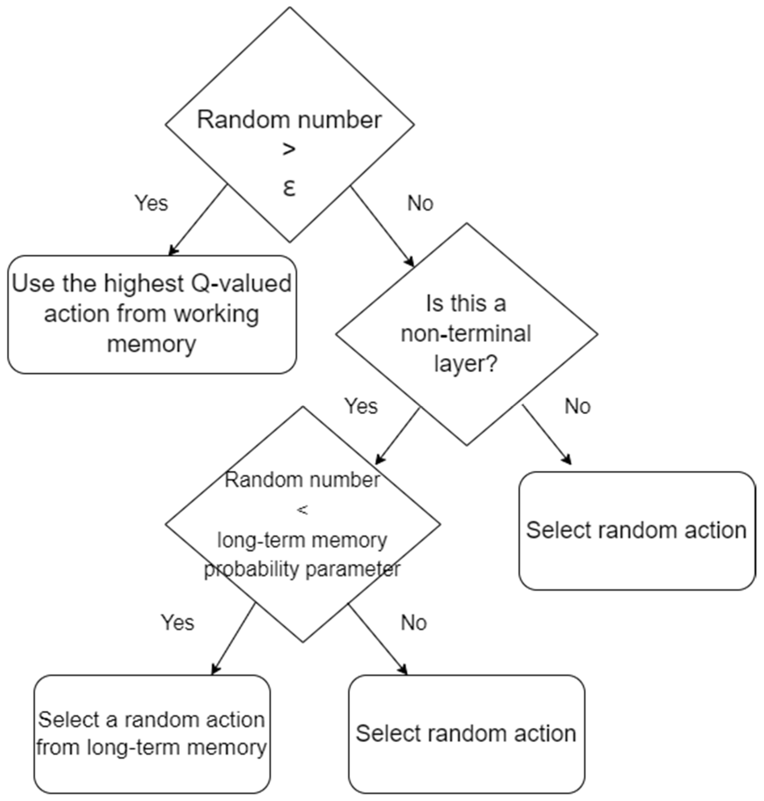
The CLL with Q-learning procedure for action selection follows the standard Q-learning protocol, but with a few changes. First, at the end of a layer, each state’s state–action pairs with the highest Q-value are copied from the Q-table to the long-term memory. Next, during an agent’s step, if a random number is greater than the epsilon greedy value, then the action with the highest Q-value is selected from the Q-table/working memory and its Q-value is modified based on its resulting rewards; otherwise, a random action is performed in non-terminal layers. In the terminal layer, if a random number is less than the long-term memory probability parameter then a random action from the state’s long-term memory is selected, otherwise, a completely random action is selected. Figure 7 contains a decision tree of the action-selection process of CLL with Q-learning.

The CLL with Q-learning procedure is as follows:

• Each agent’s sole Q-table/working and long-term memories (state–action hashmaps) are initialized as empty.
• The current layer is initialized, updating the agents’ subtask, the agents’ scenario, and the layer’s halting condition.
• The agents iterate through training episodes until the layer’s halting condition is satisfied.
  • At each step when the agent must make a decision, it generates a random number between zero and one. If that random number is greater than the epsilon value, then the agent performs the highest state’s Q-valued action from the Q-table/working memory; otherwise:
    • In all non-final layers, an action is randomly selected and the working memory/Q-table is updated based on the selected action’s returned reward.
    • In the final layer, the agent generates a random number between zero and one. If the random number is less than the long-term memory probability parameter, then the agent performs a random action that matches the current state from long-term memory; otherwise, the agent performs a random action and the working memory is updated with that action.
• At the end of a layer, each state’s highest state–action pairs are copied from the working memory to the long-term memory, allowing duplicates.
• Steps 2–4 are repeated until all layers have been completed, leaving each agent with a complete working and long-term memory.

In step 3, the highest Q-valued pair is exploited with “greater than epsilon”, which is equivalent to “less than 1-epsilon”, which is common in the literature. Both conditions evaluate to the same result and the former is used to match the CLL with (1+1) EA’s mutation condition.

Three trade-offs must be considered for CLL: (1) the additional memory requirements to facilitate the complementary memory, (2) the increased probability of reintroducing critical lost knowledge, and (3) the increased computational cost for accessing the added long-term memory component. In the memory case, we consider that the (1+1) EA’s working memory hash map and the Q-table’s 2D array require the same amount of storage as a non-complementary system. The difference in the complementary learning system is that it adds a new hash table to both approaches. Here, the worst case would be that each layer introduces new actions for every possible state to the long-term memory. Therefore, if the set of all possible unique states is S and the set of all layers is L, then the size of the long-term memory would be |S|*|L|, or the length of S and the length of L, at the end of the final layer. This worst-case increase in long-term memory size would mean that the (1+1) EA has new actions at every state at the end of each layer and the Q-table has a new, highest Q-valued action for every state at the end of each layer.

CLL’s goal is to reintroduce critical lost state-action mappings into a policy’s working memory and be selected for execution. In standard (1+1) EA and Q-learning, the probability of reintroducing a pair during an agent’s step is the probability of mutating/updating a pair from epsilon (M) multiplied by the number of elapsed layers (E) divided by the number of possible actions (A); a pair only has a chance of being modified back to its previous action-value if it is selected for an update and the E/|A| quotient represents the probability of selecting any previous layer’s action randomly. As a worst case, it is assumed that each layer will have a unique state–action pair, except in cases when there are more elapsed layers than possible actions. Equation (1) displays the probability of reintroducing a previous action in standard layered learning with a (1+1) EA or Q-Learning. CLL adds to this standard reintroduction probability when mutation/epsilon change is not performed and the agent uses the long-term memory probability parameter to determine if it will select a previous layer’s best pair at that step’s state. Therefore, the probability of reintroducing a previous layer’s pair is the standard learner’s probability of reintroduction plus the long-term memory probability. In other words, CLL’s probability of reintroducing a previous layer’s final pair is the probability of randomly selecting the previous pair plus the long-term memory probability parameter. The increased reintroduction probability is due to the long-term memory guaranteed to contain previous layers’ best pairs, because that is all it contains. Equation (2) captures the reintroduction probability, with T representing the long-term memory probability parameter.

$$\mathrm{P}\left(\mathrm{Reintroduction}\right)=M\frac{E}{\left|A\right|}$$

(1)

$$\mathrm{P}\left(\mathrm{Reintroduction}\right)=M\frac{E}{\left|A\right|}+T$$

(2)

The final consideration is the increased computational cost for accessing the added long-term memory component. The use of hashing data structures for the two approaches was selected for their ability to efficiently access action values from state keys at a computational analysis of O(1) per retrieval and insertion. Additionally, each action was copied from working-memory to long-term memory at the end of each layer; therefore, each layer had a runtime analysis of O(n), where n was the number of pairs in the policy. These computational and memory costs were needed to support the dual memory addition to layered learning, but come at the positive trade-off of an increased probability of reintroducing pairs critical at performing layer subtasks.

4. Results and Discussion

In 100 experiments of each algorithm, CLL showed a higher task performance than standard layered learning for both direct-policy search using the (1+1) EA and value-based search with Q-learning. Direct-policy search using CLL had an average UAV surveying task score of 0.631 (std: 0.142), compared with 0.5582 (0.964) for standard layered learning, representing a 13% increase in task proficiency and a Z-score of −4.24, a p-value below 0.0001, and an α of 0.05. For Q-learning, CLL increased the task performance from 0.3692 (0.0461) to 0.4011 (0.831), a 9% increase. These results had a Z-score of −3.363 and a p-value of 0.008 at an α of 0.05. The performance increases were due to CLL’s ability to reinsert forgotten beneficial knowledge into the policy for direct-policy search and boost utility values of vital pairs in value search.

Table 3. Average subtask performance after each layer for complementary layered learning.

Algorithm	Layer	Refuel	Take-Off and Survey	UAV Surveying Task
(1+1) EA	1	0.864	0.029	0.005
	2	0.381	0.742	0.118
	3	0.49	0.574	0.631
Q-learning	1	1.0	0.048	0.065
	2	0.0	0.819	0.129
	3	0.751	0.732	0.401

shows CLL UAV survey task performance averages and standard deviations after each layer for the (1+1) EA and Q-learning experiments, and

Table 4. The standard deviation of the subtask performance of each layer for complementary layered learning.

Algorithm	Layer	Refuel	Take-Off and Survey	UAV Surveying Task
(1+1) EA	1	0.133	0.06	0.008
	2	0.223	0.039	0.064
	3	0.223	0.096	0.142
Q-learning	1	0.0	0.061	0.13
	2	0.0	0.027	0.004
	3	0.006	0.025	0.083

shows their standard deviations.

The advantage of selecting a tested pair that helped in a subtask’s high performance occurred during the aggregated third layer, where both of the first two layers’ subtask performances converged and stabilized quickly. When comparing the decrease in performance of refueling, taking off, and surveying during the first 2000 epochs of the final layer, it was observed that CLL’s subtask performance dropped less drastically than that of layered learning. Additionally, refueling subtask performance stabilized, while take-off and survey performance gradually increased. Layered learning ended with a proficiency of 0.2888 for refueling and 0.4365 for take-off and survey. With CLL, refueling averaged 0.49 and take-off and survey averaged 0.5736 at the end of the final layer, representing 70% and 31% increases in subtask performance, respectively. These results indicate that CLL outperforms standard layered learning.

The forgetting metrics of performance difference (PD), direct forgetting metric (DFM), and maximum forgetting metric (MFM) were used to quantify how much forgetting takes place in a learner. These metrics measured the policy-performance change during a direct-policy learning process. However, Q-learning’s epsilon-greedy and probabilistic action selection did not allow the value-based learning method to be evaluated by these forgetting metrics; therefore, only the (1+1) EA forgetting measures were reported. PD measures the average overall task performance change per learning episode. DFM is the weighted performance difference between a policy p_t−1 and its immediate policy change p. MFM is the same as DFM, but policy p_t−1 is replaced with the best-performing policy between episodes 1 and t−1. DFM and MFM are increasingly proportionally weighted by the number of elapsed episodes to place higher importance on policy changes toward the end of the learning phase. DFM and MFM can be calculated at different intervals to generate observations of the time the agent can allow its policy to change before being evaluated. Therefore, PD is captured at the end of each episode; DFM Even and MFM Even calculate forgetting every two episodes, while DFM 50 and MFM 50 measure forgetting every 50 episodes. With these forgetting metrics, we can determine whether learning or forgetting occurs throughout the learning process. For example, the higher positive measurement indicates that positive learning is taking place; performance has increased on average per episode interval. Conversely, negative forgetting is more prevalent if the measured value is negative and overall performance is stunted per measured interval.

Layered learning received a negative forgetting score of −0.1514 (0.1164) for MFM Even while CLL scored −0.1146 (0.07915). A two-tailed Z-test with an α of 0.05 showed that CLL’s negative forgetting decrease was significant with a Z-value of −2.6145 and a p-value of 0.0089. MFM 50 provided the same conclusion that CLL’s negative forgetting was lessened: Layered learning’s MFM 50 score was −0.1139 (0.087) and CLL produced −0.0864 (0.5904), with a Z-value of −2.6155 and a p-value 0.0089.

Table 5. EA forgetting metrics for standard vs. complementary layered learning.

Forgetting Metric	Layered Learning	Complementary Layered Learning
PD	0.00002	0.00002
DFM Even	0.00001	0.00002
MFM Even	−0.15143	−0.111462
DFM 50	0.00001	0.00002
MFM 50	−0.11385	−0.08635

displays all the forgetting metric results of the direct-policy experiments.

The decrease in negative forgetting experienced by CLL is directly related to the number of pairs restored in the final layer. During Layer 1’s optimization of the refueling subtask, CLL reverted 3.67 pairs to their Layer 1 mapping in Layer 2, resulting in a 194% increase over layered learning’s 1.25 restorations per policy. Additionally, it should be noted that layered learning averaged 14.58 (4.6478) pair changes from Layer 1 to Layer 2. The increase in restored pairs that were reverted to their mappings originally found in Layer 1 led to an increase in the probability that some of those relearned pairs were beneficial knowledge to the refueling subtask and aided in its performance at the end of learning.

To further compare layered learning to CLL under direct-policy search, transfer learning metrics, such as transfer regret, transfer ratio, and calibrated transfer ratio, were used. These metrics confirmed that in the experiments, CLL outperformed layered learning. An abbreviated form of these metrics was used for the comparison between EA and Q-learning algorithms by sampling overall task performance at three critical points of learning: the end of each layer. The transfer ratio was 1.1026, favoring the CLL experimental approach because its performance integral ratio was greater than 1. Both transfer ratio (0.1127) and calibrated transfer ratio (0.0323) also indicated that better performance occurred in CLL because their values were greater than zero. CLL improved standard layered learning from each of these measures and clearly made measurable progress in mitigating the stability–plasticity imbalance. The transfer metrics also confirmed the improvement of CLL over standard layered learning in direct-policy search under (1+1) EA, with a transfer ratio of 1.0923, a transfer regret of 0.1189, and a calibrated transfer ratio of 0.0205. These results confirmed that under these experimental conditions and overall task, CLL improved standard layered learning in both direct policy and value search.

Overall, the complementary learning system’s augmentation to layered learning improved task performance in the final layer. By updating the Q-table based on averages from the indexed collection, the policy increased the chance to reevaluate beneficial pairs that saw their Q-values decrease due to the take-off and survey layer. The (1+1) EA followed a similar protocol by either directly copying an action from the long-term memory, randomly selecting an action from a matching state’s pair in the long-term memory, or completely generating a new random action. By seeding a policy with long-term memory knowledge in its last learning phase, the learner had a final chance to reintroduce discarded knowledge—but this time, in the context of the overall task.

5. Conclusions

In this work, the task decomposition-based transfer learning paradigm of layered learning proved to be susceptible to a stability–plasticity imbalance. The imbalance was causing machine learning implementations of the paradigm to lose critical knowledge as the learner optimized its policy on new tasks. Consequently, the occurrence of catastrophic forgetting caused layered learners to perform suboptimally and waste learning time because key knowledge was driven or drifted out of the policy and, potentially, was never regained.

This work extends previous forgetting studies in layered learning to combat the stability–plasticity imbalance. First, this study examined the causes of catastrophic forgetting in value-based policy searches, extending previous forgetting demonstrations with direct-policy searches. This work highlights layered learning’s performance challenges in intentionally designed theoretical single-policy and real-world, multi-agent problems. Second, this work outlined existing solutions to catastrophic forgetting in other transfer learning approaches, including successful uses of complementary memory systems in biological and artificial neural networks. Finally, this work proposed complementary layered learning as a new extension to the transfer learning paradigm of layered learning. Other dual memory approaches inspired this augmentation to standard layered learning. Uniquely, complementary layered learning stores a history of state–action pairs into a long-term memory gained from all layers, excluding the final layer. In the last layer, the policy probabilistically reintroduces pairs into the policy (working memory) or generates a new state–action mapping, based on a controllable long-term memory exploitation parameter. Supported by this work’s experiment results, complementary layered learning significantly improved learning performance in direct-policy and value-based searches. Importantly, the new augmentation reduces the number of training episodes necessary to regain lost knowledge. Further, adding a long-term memory allowed the policy to retain knowledge that could normally be discarded forever in standard layered learning.

Now that layered learning has been enhanced to balance stability and plasticity in simulated agents and under theoretical scenarios, future work will evaluate the complementary system within physical robotic learners. Traditional challenges with real robots are their limited memory capacity and computational ability. The advantages with the direct-policy and value-based searches implemented in this work are their explainability and their low-resource requirements for dual memories, training, and decision-making. Therefore, training robots with the enhanced learning paradigm has the potential to elevate their current capability, but first, it is necessary to understand the feasibility and limitations of complementary layered learning in such real, physical learning systems.