Supervised Contrastive Learning for Voice Activity Detection

Abstract

The noise robustness of voice activity detection (VAD) tasks, which are used to identify the human speech portions of a continuous audio signal, is important for subsequent downstream applications such as keyword spotting and automatic speech recognition. Although various aspects of VAD have been recently studied by researchers, a proper training strategy for VAD has not received sufficient attention. Thus, a training strategy for VAD using supervised contrastive learning is proposed for the first time in this paper. The proposed method is used in conjunction with audio-specific data augmentation methods. The proposed supervised contrastive learning-based VAD (SCLVAD) method is trained using two common speech datasets and then evaluated using a third dataset. The experimental results show that the SCLVAD method is particularly effective in improving VAD performance in noisy environments. For clean environments, data augmentation improves VAD accuracy by 8.0 to 8.6%, but there is no improvement due to the use of supervised contrastive learning. On the other hand, for noisy environments, the SCLVAD method results in VAD accuracy improvements of 2.9% and 4.6% for “speech with noise” and “speech with music”, respectively, with only a negligible increase in processing overhead during training.

1. Introduction

Voice activity detection (VAD) is an essential preprocessing stage for various audio-signal-related downstream applications. It is a binary classification task that distinguishes an audio signal into two classes consisting of “speech” and “non-speech”. VAD classification of input audio signals is performed prior to various audio-related downstream tasks, thereby possibly improving the performance and efficiency of those tasks.

Early VAD research works were conducted based on statistical models [1,2]. Recently, deep learning-based VAD models leveraging various neural network models have been actively explored, including convolutional neural networks (CNN) [3,4,5,6,7], recurrent neural networks (RNN), and long short-term memory (LSTM) networks [8,9,10,11]. In particular, Jia et al. and Kopuklu et al. [4,5] proposed compact VAD models suitable for use in a limited hardware resource environment. In the case of [4], the model size was about 10 times smaller than that of other CNN-based models [3] using 1D time-channel separable convolution but the VAD performance was similar. In the case of [5], a raw audio signal was used as input and the model size was reduced by utilizing depthwise-separable convolution and point-wise group convolution.

Since VAD is a fundamental initial task that is essential for processing audio signals in all types of real environments, research on a noise-robust VAD model is an important topic in its own right. In [12], a method utilizing data augmentation and knowledge distillation was proposed for VAD with robust classification accuracy in a noisy environment.

Methods using contrastive learning have been proposed to further improve classification performance and noise robustness in other audio-signal-related classification tasks such as keyword spotting and environmental sound classification [13,14,15]. Contrastive learning is a method that is mainly used in self-supervised representation learning. It aims to narrow the distance between positive pair samples, i.e., the samples in the same class, and widen the distance between negative pair samples, i.e., the samples in different classes, using a contrastive loss function. In [14], the authors improved the noise robustness of the keyword spotting model by applying a new loss function, which was based on a contrastive loss function, to the keyword spotting task.

Supervised contrastive learning [15], first proposed for use in image classification tasks, was suggested as a modified contrastive loss function that allows contrastive learning to be used in a supervised setting. For audio-signal-related tasks, Nasiri et al. [13] proposed applying supervised contrastive learning with various data augmentation methods to environmental sound classification.

Previous research works have been conducted to improve noise robustness in audio-related tasks, such as keyword spotting and environmental sound classification, through the utilization of contrastive learning [14] and supervised contrastive learning [13]. However, there have been no publicly published works where these methods have been applied and experimentally proven to be effective for VAD. Thus, this paper has implemented and investigated the effectiveness of supervised contrastive learning for the VAD task. The experimental results are very interesting in that supervised contrastive learning has been found to improve the effectiveness of VAD in noisy environments but is essentially ineffective in clean sound environments. In addition, for both clean and noisy environments, data augmentation can improve VAD accuracy provided that effective sound-related data augmentation methods are used. In this paper, a new supervised contrastive learning-based voice activity detection (SCLVAD) model training strategy, which can improve the model’s performance for noisy audio signals, is proposed.

In the proposed SCLVAD strategy, various new positive and negative pairs are generated using SpecAugment [16] and Cutout for spectrogram [4,17], which are data augmentation methods that have been specifically developed for audio signal processing. These new positive and negative pairs are added to an existing speech dataset during the neural network training process. Then, for the loss function, the supervised contrastive loss is combined with the cross-entropy loss in a weighted manner, as originally suggested in [13].

MarbleNet, proposed in [4], was used as the baseline model and experiments were conducted to evaluate the performance of the proposed method. Based on the model evaluation method used in [4], the performance of the baseline MarbleNet model and the MarbleNet model trained with the proposed SCLVAD strategy were evaluated and compared. The AVA-Speech dataset [18] was used as the test dataset and the true-positive rate (TPR) and the area under the receiver operating characteristic (AUROC) curve were used as the main evaluation metrics.

2. Background and Related Work

In this section, the background knowledge and related works on VAD and supervised contrastive learning are explained. The main features of the related works and their pros and cons are summarized in

Table 1. A list of related methods and their key features, pros, and cons.

Method	Pros	Cons	Features
MarbleNet [4]	Compact model size	Lack of noise robustness	1D time-channel separable convolution
CNN-TD [3]	High classification accuracy	Large model size	VGG-16-based neural network
Supervised contrastive learning [15]	Highly improves classification accuracy	Additional neural network	Modified contrastive learning to use labeled dataset
SoundCLR [13]	High classification accuracy	Additional neural network	Supervised contrastive learning for environmental sound classification task

.

2.1. Voice Activity Detection

VAD is a binary classification task that distinguishes a given audio signal into speech and non-speech classes. VAD is an essential and fundamental preprocessing step for audio-signal-related downstream applications such as keyword spotting and automatic speech recognition. Therefore, by performing accurate VAD on the input audio signal before the various downstream tasks, the efficiency of the subsequent tasks can be improved. In other words, if VAD is not performed properly, the performance of the subsequent tasks can be degraded, making the classification performance of VAD very important.

Recently, research on deep learning-based VAD models using various neural networks has been actively conducted. In [4], the authors suggested a compact, yet high-performance VAD model named MarbleNet, considering the use of the VAD model in a limited hardware resource environment. Using 1D time-channel separable convolution, MarbleNet has approximately 10 times fewer parameters than other CNN-based models such as CNN-TD [3] but the performance was comparable.

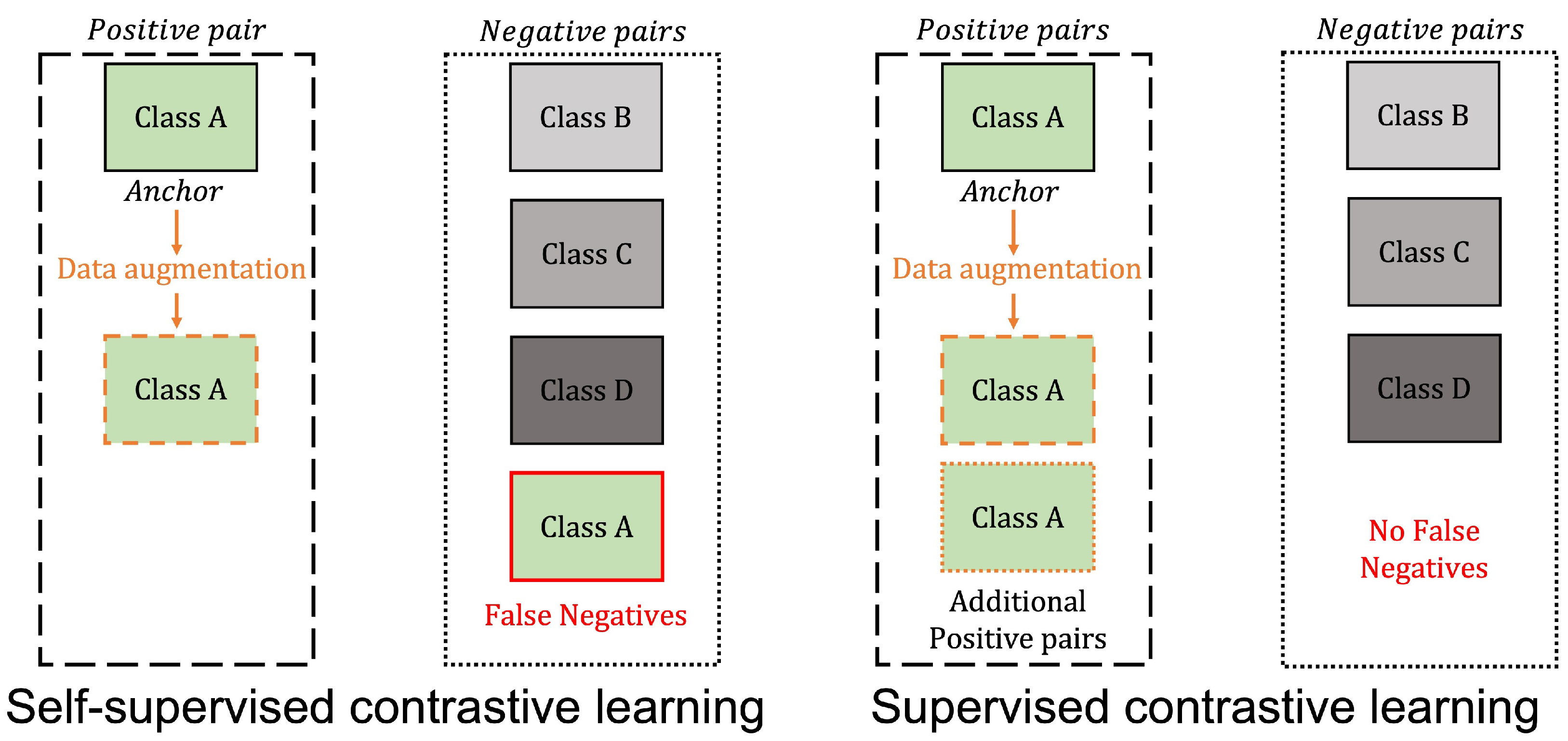
2.2. Supervised Contrastive Learning

As shown in Figure 1, supervised contrastive learning is a modified method that allows self-supervised contrastive learning to be used in fully supervised settings. Here, an anchor refers to the sample that is used as the basis for that class. Given a specific anchor, a positive pair refers to another sample belonging to the same class as the anchor and a negative pair refers to a sample belonging to a class that is different from that of the anchor. Self-supervised contrastive learning utilizes only one positive pair. However, supervised contrastive learning leverages all data belonging to the same class as an anchor within a given batch as positive pairs. Since the label information of the dataset can be utilized, false negatives do not occur. Supervised contrastive learning was first applied to the existing supervised learning-based image classification task to improve classification performance [15]. In the case of audio-signal-related tasks, a supervised contrastive loss function combined with a cross-entropy loss function was applied to environmental sound classification [13]. Classification performance was improved by applying a combined loss function, along with various data augmentation methods.

Similar to contrastive learning, supervised contrastive learning pulls an anchor and positive pairs closer together and pushes negative pairs farther away from an anchor in the embedding space. In contrastive learning, since there is no label information for the dataset in the self-supervised setting, only one positive pair is generated using data augmentation and negative pairs are randomly selected within the minibatch. Therefore, a false-negative problem may occur in which the selected negative pairs belong to the same class as the anchor. However, the supervised contrastive learning method has the advantage of selecting negative pairs without a false-negative problem by leveraging the label information. In addition, since all samples belonging to the same class as the anchor within the minibatch can be used as positive pairs, the relationships between more sample pairs can be reflected in the loss function.

3. Proposed Method

In the proposed SCLVAD model training strategy, the VAD model is trained using a supervised contrastive loss function combined with a cross-entropy loss function, as originally suggested in [13], along with various data augmentation methods. The structure of the proposed SCLVAD training strategy is illustrated in Figure 2.

A batch of input data is augmented using data augmentation methods, such as SpecAugment [16] and Cutout for spectrogram [4,17], which are specialized for audio signal data. During the training process, since both the projection layer and classification layer are used, the supervised contrastive loss and cross-entropy loss can be calculated simultaneously as the batch of input data propagates.

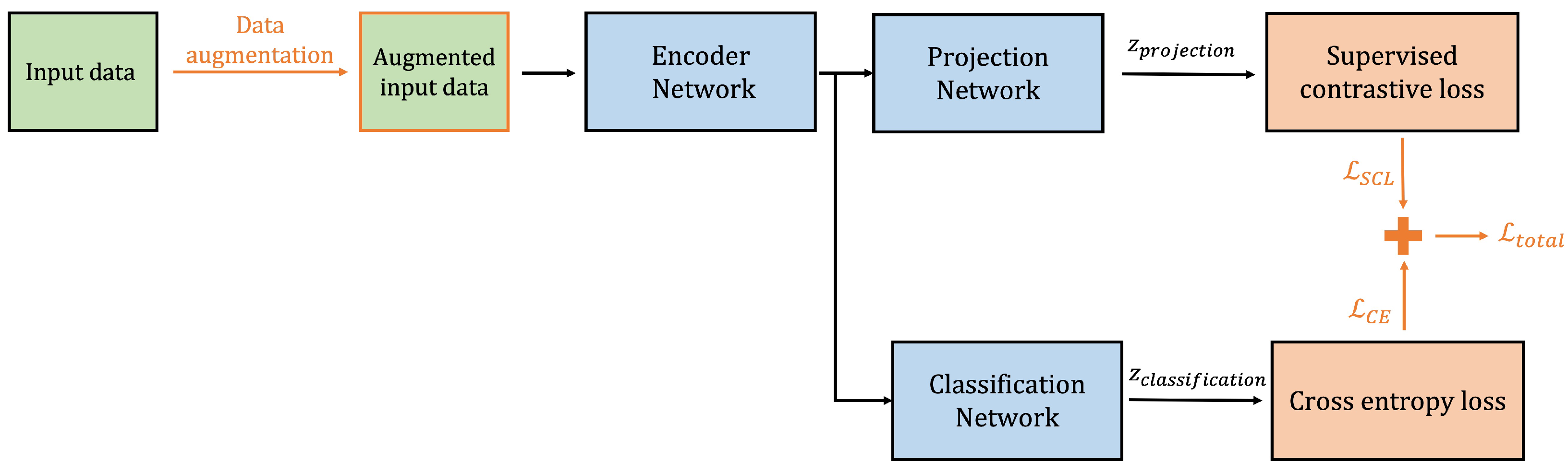
3.1. Proposed Supervised Contrastive Learning-Based Voice Activity Detection Algorithm

In the proposed SCLVAD training strategy, shown in Algorithm 1, the method consists of a data augmentation process and training with two loss functions. For one batch of input data with N samples, the original samples ${\left\{x_{original}^i\right\}}_{i=1}^N$ are augmented into ${\left\{x_{augmented}^i\right\}}_{i=1}^N$ through the augmentation process $Augment\left(\right)$. Then, the encoder network ${\mathcal{N}}_{encoder}$ receives ${\left\{x_{augmented}^i\right\}}_{i=1}^N$, which is an augmented batch, and outputs ${\left\{e^i\right\}}_{i=1}^N$, which is the embedding feature. The projection network ${\mathcal{N}}_{projection}$ and classification network ${\mathcal{N}}_{classification}$ receive ${\left\{e^i\right\}}_{i=1}^N$ as an input and output the projection output ${\left\{z_{projection}^i\right\}}_{i=1}^N$ and classification output ${\left\{z_{classification}^i\right\}}_{i=1}^N$, respectively. Finally, the supervised contrastive loss ${\mathcal{L}}_{SCL}$ and cross-entropy loss ${\mathcal{L}}_{CE}$ are calculated by ${\left\{z_{projection}^i\right\}}_{i=1}^N$ and ${\left\{z_{classification}^i\right\}}_{i=1}^N$ to update each neural network.

Algorithm 1 Supervised Contrastive Learning for Voice Activity Detection—Model Training Strategy

Input: Encoder network ${\mathcal{N}}_{encoder}$, projection network ${\mathcal{N}}_{projection}$, classification network ${\mathcal{N}}_{classification}$, Hyperparameters, Dataset samples Output: Optimized encoder network ${\mathcal{N}}_{encoder}^{optimized}$ and classification network ${\mathcal{N}}_{classification}^{optimized}$ Initialize: Initialization of encoder network ${\mathcal{N}}_{encoder}$, projection network ${\mathcal{N}}_{projection}$, classification network ${\mathcal{N}}_{classification}$ 1: for $l=1,2,\cdots ,totalepochs$  do 2:       for $m=1,2,\cdots ,totalbatches$ do 3:             Generate a batch of input data using data augmentation methods: 4:                       ${\left\{x_{augmented}^i\right\}}_{i=1}^N\leftarrow Augment\left({\left\{x_{original}^i\right\}}_{i=1}^N\right)$; 5:             Input the augmented data to the encoder network: 6:                       ${\left\{e^i\right\}}_{i=1}^N\leftarrow {\mathcal{N}}_{encoder}\left({\left\{x_{augmented}^i\right\}}_{i=1}^N\right)$; 7:             Input the embedding to the projection network and classification network: 8:                       ${\left\{z_{projection}^i\right\}}_{i=1}^N\leftarrow {\mathcal{N}}_{projection}\left({\left\{e^i\right\}}_{i=1}^N\right)$; 9:                       ${\left\{z_{classification}^i\right\}}_{i=1}^N\leftarrow {\mathcal{N}}_{classification}\left({\left\{e^i\right\}}_{i=1}^N\right)$; 10:             Calculate the supervised contrastive loss using Equation (2): ${\mathcal{L}}_{SCL}$; 11:             Calculate the cross-entropy loss using Equation (1): ${\mathcal{L}}_{CE}$; 12:             Calculate the total loss using Equation (3): ${\mathcal{L}}_{total}$; 13:             Update the projection network ${\mathcal{N}}_{projection}$, classification network ${\mathcal{N}}_{classification}$, and encoder network ${\mathcal{N}}_{encoder}$; 14:       end for 15: end for

At the inference process after the training process, the projection layer ${\mathcal{N}}_{projection}$ is detached and only the encoder network ${\mathcal{N}}_{encoder}$ and classification network ${\mathcal{N}}_{classification}$ are used for the VAD classification. Instead of two-stage training, which first trains the encoder network ${\mathcal{N}}_{encoder}$ and then fine-tunes the classification network ${\mathcal{N}}_{classification}$, as suggested in [15], one-stage training was applied using both the projection network ${\mathcal{N}}_{projection}$ and the classification network ${\mathcal{N}}_{classification}$ simultaneously, as suggested in [13]. Detailed descriptions of the loss functions are described in the next part of this section.

3.2. Loss Functions

In the proposed algorithm, two loss functions are used to train the VAD model, as suggested in [13]. The first loss function is the cross-entropy loss function ${\mathcal{L}}_{CE}$. In many VAD-related studies [3,4,5,12], a cross-entropy loss has been used to train VAD models. The cross-entropy loss is calculated using the output probability distribution of the neural network of the input samples and the true probability distribution of those samples. The training of the neural network model using a cross-entropy loss aims to reduce the entropy between the two probability distributions. The true probability distribution can be expressed as one-hot vectors from labels and represents the class of samples. Therefore, the cross-entropy loss function for the proposed SCLVAD algorithm can be expressed as follows:

$${\mathcal{L}}_{CE}=\mathcal{H}(p,z)=-\sum _i{p}^{i}log\left(z_{classification}^i\right)$$

(1)

where $p^i$ indicates the true probability distribution and $z_{classification}^i$ is the output probability distribution of the classification network ${\mathcal{N}}_{classification}$.

The second loss function is the supervised contrastive loss function ${\mathcal{L}}_{SCL}$. As shown in Algorithm 1, N samples in one batch for the original dataset can be represented as ${\left\{x_{original}^i\right\}}_{i=1}^N$ and augmented samples can be represented as ${\left\{x_{augmented}^i\right\}}_{i=1}^N$. The labels of $x_{original}^i$ and $x_{augmented}^i$ are the same and can be expressed as $y^i$. When $x_{augmented}^i$ is forward propagated to the encoder network and projection network, the projection network outputs $z_{projection}^i$. Therefore, the supervised contrastive loss for the proposed SCLVAD algorithm can be expressed as follows:

$${\mathcal{L}}_{SCL}=-\frac{1}{N_{pos}^i}\sum _{p\in P\left(i\right)}log\frac{exp(z_{projection}^i·z_{projection}^p/\tau )}{{\sum }_{k\in K\left(i\right)}exp(z_{projection}^i·z_{projection}^k/\tau )}$$

(2)

where $\tau$ is a scalar value, which is a temperature parameter, and the sample with the index i is an anchor. $K\left(i\right)$ is the set of samples excluding i among the total N samples and $P\left(i\right)$ is the set of positive samples. Finally, $N_{pos}^i$ is the number of positive samples with the same label as the anchor, $y^i$.

Therefore, the final loss function for the training process of the proposed SCLVAD method consists of the aforementioned Equations (1) and (2), which can be expressed as follows:

$${\mathcal{L}}_{total}=\alpha {\mathcal{L}}_{CE}+\beta {\mathcal{L}}_{SCL}$$

(3)

where $\alpha$, $\beta$ are the coefficients for each loss function. Each coefficient is used as a hyperparameter to adjust the weight of each loss function.

4. Experiments

In this section, the implementation details of the neural network model and the experimental results are explained. All the experiments were conducted on an NVIDIA GeForce RTX 2080 Ti GPU with a PyTorch [19] machine learning framework. More details of the neural network models and datasets used for the experiments are explained in the following sections.

4.1. Implementation Details

For a fair comparison, the same MarbleNet architecture was used for both the baseline and the SCLVAD methods. The training parameters, such as the batch size and number of training epochs, were applied equally to both methods, as in [4].

For both the baseline and SCLVAD models, a total of 150 epochs of training were performed and the stochastic gradient descent (SGD) optimizer [20] with a momentum of $0.9$ and weight decay of $1\times {10}^{-3}$ was used. The initial learning rate was $1\times {10}^{-2}$ and the Warmup-Hold-Decay learning rate scheduler [21] was used. Batch sizes of 256 and 512 were used for the experiments.

For the proposed SCLVAD algorithm, the temperature $\tau$ for ${\mathcal{L}}_{SCL}$ in Equation (2) was $0.07$. The coefficients $\alpha$ and $\beta$ for ${\mathcal{L}}_{total}$ in Equation (3) were both $0.5$, as used in [13]. The encoder network ${\mathcal{N}}_{encoder}$, the encoder part of MarbleNet, which is part of the last two fully connected layers, was excluded. The classification network ${\mathcal{N}}_{classification}$ was the last two fully connected layers of MarbleNet. The structures of ${\mathcal{N}}_{encoder}$ and ${\mathcal{N}}_{classification}$ were the same as in MarbleNet and [4]. The projection network ${\mathcal{N}}_{projection}$ was located after the encoder network ${\mathcal{N}}_{encoder}$ and was parallel with the classification network ${\mathcal{N}}_{classification}$, as shown in Figure 2. The structure of ${\mathcal{N}}_{projection}$ consisted of two fully connected layers and a ReLU activation function. The sizes of the input and output of the first fully connected layer were both 128 and the sizes of the input and output of the second fully connected layer were 128 and 64, respectively. The final output was normalized and used for computing ${\mathcal{L}}_{SCL}$.

4.2. Training Dataset

The training dataset was a variant of the training dataset that was used in [4]. The dataset corresponding to the ‘speech’ class was composed of the Google Speech Commands Dataset V2 [22] and the ‘non-speech’ class was composed of audio samples from freesound.org (accessed on 26 January 2023) [23]. The Google Speech Commands Dataset V2 consists of 105,000 speeches of about 1s lengths and includes 35 classes of utterances such as “On”, “Right”, and “Go”. The total number of audio samples from freesound.org was 2615 and 32 classes of background noise were used, where the length of each sample varied from 0.63 s to 100 s.

Due to the different lengths of the initial audio samples, the audio samples were preprocessed in order to produce training audio samples of the same length, as conducted in [4]. The audio samples were converted into segments of 0.63-second lengths using this process. Then, a 64-dimensional mel frequency cepstral coefficient (MFCC) encoding of this data was used as the training input for the MarbleNet neural network.

MFCC is an audio feature representation commonly used in speech and audio signal processing. It is a set of coefficients that describes the shape of a signal’s power spectrum in a way that more closely resembles the way the human auditory system perceives sound. MarbleNet [4], which was the baseline neural network architecture used in the experiments, also uses MFCC features instead of the Mel spectrogram. The experimental results presented in [4] showed that the accuracy achieved using MFCC was higher than the corresponding accuracy using the Mel spectrogram. Therefore, in this paper, MFCC was used to produce the training input features and the resulting performance was compared with the baseline.

4.3. Performance Evaluation

In order to ensure a proper evaluation of the effectiveness of the proposed method, testing was conducted using the AVA-Speech dataset [18], which is a completely different dataset from the datasets used during training (sound samples from Google Speech Commands dataset and freesound.org were used during training). The use of the AVA-Speech dataset for testing enabled a fair comparison with MarbleNet since MarbleNet also used the AVA-Speech dataset for testing [4]. The AVA-Speech dataset is composed of YouTube videos with four classes: “no speech”, “clean speech”, “speech with noise”, and “speech with music”. As in [4], the “All” speech class, which is a combination of the aforementioned three speech classes, was also used for the evaluation.

Two metrics were used to evaluate and compare the proposed method with the MarbleNet baseline. As the first evaluation metric, the true-positive rate (TPR) was calculated at the frame level for each speech class, and the TPR value when the false-positive rate (FPR) = 0.315 was used (this evaluation method is the same one used in MarbleNet). For the second evaluation metric, the area under the receiver operating characteristic (AUROC) curve was used. This is a metric commonly used to measure the overall effectiveness of speech processing.Sentences have been revised

In the evaluation process, two frame-level prediction methods were evaluated. First, the frame was created by shifting the window for 10 ms without overlapping and then, the window’s prediction was used to indicate the label of the frame. Second, the prediction was created by overlapping the input segments. The label for the frame spanned by multiple segments was generated by applying a smoothing filter, which used the median values. The degree of overlapping was fixed at 87.5%.

4.4. Data Augmentation

Four audio data augmentation methods, including time shift, white noise augmentation, SpecAugment [16], and Cutout [17], were used in [4]. These augmentation methods were applied to both the baseline and the proposed training algorithm. White noise augmentation was applied with a probability of 80% and the other aforementioned augmentation methods were applied to every training dataset. The parameters related to augmentation were set in the same way as [4]. Specifically, time shift was applied in the range of −5 ms to 5 ms and white noise with a magnitude between −90 dB and −46 dB was applied for white noise augmentation. For SpecAugment, two continuous time masks with sizes ranging from 0 to 25 time steps were used and two continuous frequency masks with sizes ranging from 0 to 15 frequency bands were used. For Cutout, five rectangular masks were used in the time and frequency dimensions. Each mask contained a width of 25 time steps and a height of 15 frequency bands.

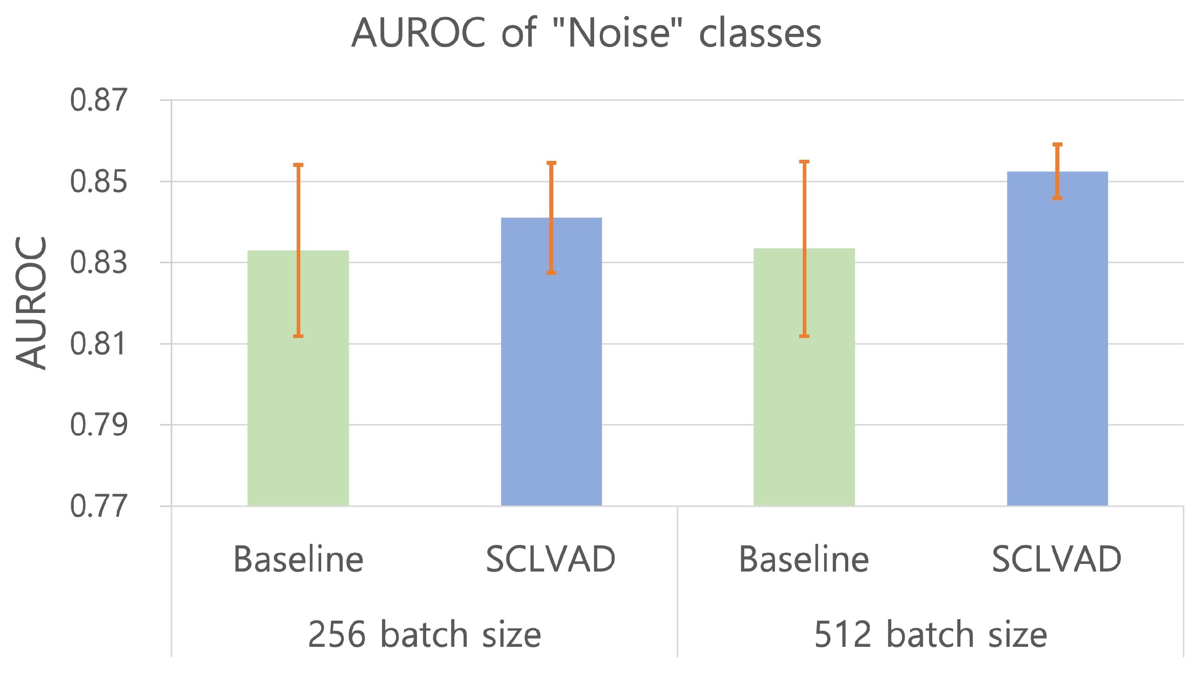
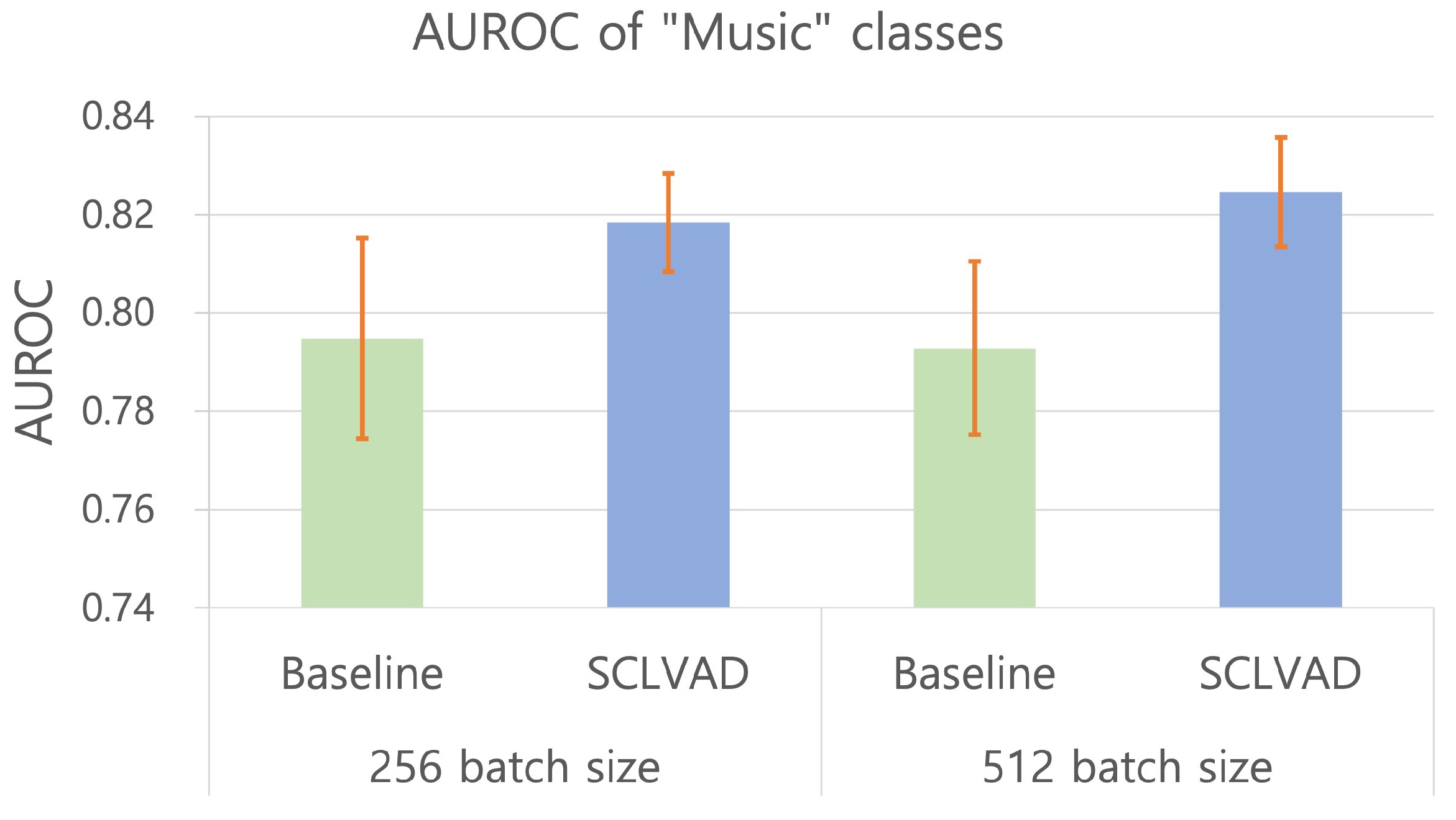
4.5. Experimental Results

Three different training methods are compared to verify the effectiveness of the proposed method.

In

Table 2. Experimental results of the baseline and SCLVAD algorithm with a batch size of 256.

Batch Size = 256	TPR for FPR = 0.315				AUROC
Method	Clean	Noise	Music	All	All
No Augmentation	$0.888\pm 0.021$	$0.683\pm 0.028$	$0.655\pm 0.021$	$0.729\pm 0.023$	$0.778\pm 0.014$
Baseline [4]	$\mathbf{0}.\mathbf{960}\pm 0.011$	$0.794\pm 0.023$	$0.742\pm 0.028$	$0.823\pm 0.021$	$0.844\pm 0.017$
SCLVAD	$0.959\pm \mathbf{0}.\mathbf{009}$	$\mathbf{0}.\mathbf{807}\pm \mathbf{0}.\mathbf{018}$	$\mathbf{0}.\mathbf{779}\pm \mathbf{0}.\mathbf{012}$	$\mathbf{0}.\mathbf{839}\pm \mathbf{0}.\mathbf{015}$	$\mathbf{0}.\mathbf{851}\pm \mathbf{0}.\mathbf{009}$

and

Table 3. Experimental results of the baseline and SCLVAD algorithm with a batch size of 256 and input segments overlapped by 87.5%.

Batch Size = 256	TPR for FPR = 0.315				AUROC
Method	Clean	Noise	Music	All	All
No Augmentation + overlap 87.5%	$0.892\pm 0.021$	$0.687\pm 0.030$	$0.661\pm 0.023$	$0.734\pm 0.025$	$0.783\pm 0.016$
Baseline + overlap 87.5% [4]	$0.969\pm 0.011$	$0.808\pm 0.025$	$0.758\pm 0.026$	$0.838\pm 0.021$	$0.854\pm 0.018$
SCLVAD + overlap 87.5%	$\mathbf{0}.\mathbf{969}\pm \mathbf{0}.\mathbf{008}$	$\mathbf{0}.\mathbf{825}\pm \mathbf{0}.\mathbf{019}$	$\mathbf{0}.\mathbf{793}\pm \mathbf{0}.\mathbf{013}$	$\mathbf{0}.\mathbf{857}\pm \mathbf{0}.\mathbf{013}$	$\mathbf{0}.\mathbf{863}\pm \mathbf{0}.\mathbf{011}$

, No Augmentation indicates MarbleNet trained without using either the data augmentation methods or the proposed SCLVAD algorithm. The other two methods, baseline and SCLVAD, were trained using the same augmentation methods. Baseline indicates MarbleNet trained without the proposed SCLVAD algorithm and SCLVAD indicates MarbleNet trained with the proposed SCLVAD algorithm.

In addition, the evaluation of each method with segment overlapping is reported. For the overlapped case in Table 3 and Table 5, the input segment was overlapped by 87.5%, leveraging the median smoothing filter. All the values in the table are the mean and standard deviation values of five repeated experiments for each case. More specifically, each value in the table indicates the $mean\pm standarddeviation$.

The experimental results using a batch size of 256 are reported in Table 2 and Table 3. In both cases, MarbleNet trained without the data augmentation methods showed the worst classification performance for all speech classes. Although the performance improved when data augmentation was applied, there was a greater performance improvement when the proposed method and data augmentation were used together.

For the most part, SCLVAD achieved superior results both with and without the segments overlapping to the baseline. With the SCLVAD method, the AUROC of MarbleNet for the “All” class was improved by 0.9% with overlapping segments compared to the baseline. For the TPR with the overlapping segments, the improvements were 1.7%, 3.5%, and 1.9% for the “Noise”, “Music”, and “All” classes, respectively. Moreover, the standard deviations for all cases were significantly reduced using SCLVAD. For “Clean” speech, the mean TPR values of SCLVAD and MarbleNet were similar but SCLVAD showed a smaller standard deviation value. From these results, it can be seen that SCLVAD more robustly distinguished between “speech” and “non-speech” in terms of noise. Considering the fact that SCLVAD barely affected the performance for the “Clean” speech data but significantly improved the performance for the other classes, the proposed method can provide robustness for noisy data. In addition, SCLVAD can help to obtain stable training results. This can be seen in the standard deviation results shown in Table 2, Table 3,

Table 4. Experimental results of the baseline and SCLVAD algorithm with a batch size of 512.

Batch Size = 512	TPR for FPR = 0.315				AUROC
Method	Clean	Noise	Music	All	All
Baseline [4]	$0.960\pm 0.012$	$0.793\pm 0.027$	$0.739\pm 0.029$	$0.821\pm 0.024$	$0.845\pm 0.016$
SCLVAD	$\mathbf{0}.\mathbf{961}\pm \mathbf{0}.\mathbf{003}$	$\mathbf{0}.\mathbf{819}\pm \mathbf{0}.\mathbf{012}$	$\mathbf{0}.\mathbf{786}\pm \mathbf{0}.\mathbf{012}$	$\mathbf{0}.\mathbf{849}\pm \mathbf{0}.\mathbf{010}$	$\mathbf{0}.\mathbf{859}\pm \mathbf{0}.\mathbf{005}$

and

Table 5. Experimental results of the baseline and SCLVAD algorithm with a batch size of 512 and input segments overlapped by 87.5%.

Batch Size = 512	TPR for FPR = 0.315				AUROC
Method	Clean	Noise	Music	All	All
Baseline + overlap 87.5% [4]	$0.966\pm 0.013$	$0.806\pm 0.028$	$0.748\pm 0.026$	$0.834\pm 0.025$	$0.854\pm 0.018$
SCLVAD + overlap 87.5%	$\mathbf{0}.\mathbf{972}\pm \mathbf{0}.\mathbf{003}$	$\mathbf{0}.\mathbf{837}\pm \mathbf{0}.\mathbf{013}$	$\mathbf{0}.\mathbf{804}\pm \mathbf{0}.\mathbf{018}$	$\mathbf{0}.\mathbf{865}\pm \mathbf{0}.\mathbf{010}$	$\mathbf{0}.\mathbf{871}\pm \mathbf{0}.\mathbf{006}$

.

Since SCLVAD uses supervised contrastive learning, the performance can be improved as the number of negative pairs increases [15]. Therefore, the performance of SCLVAD was also tested with a batch size of 512 while maintaining the other hyperparameters. In addition, for a fair comparison, the performance was compared by applying the same batch size to the MarbleNet baseline model.

As shown in Table 4 and Table 5, SCLVAD showed a higher TPR and AUROC for all speech classes compared to the baseline. In the case of the baseline, as the batch size increased, the AUROC was similar but the TPR degraded for all speech classes. However, in the case of SCLVAD, both the AUROC and TPR improved as the batch size increased. In addition, the overall standard deviation was further reduced, resulting in improved model stability as the batch size increased. With the proposed SCLVAD method, the AUROC of the MarbleNet for the “All” class was improved by 1.7% with overlapping segments compared to the baseline trained with a batch size of 256, which showed better performance than the baseline trained with a batch size of 512. For the TPR with overlapping segments, the improvements were 2.9%, 4.6%, and 2.7% for the “Noise”, “Music”, and “All” classes, respectively.

In order to provide a more detailed analysis, we examined the AUROC values, as well as the TPR values, for the “Noise” and “Music” classes when the input segments overlapped by 87.5%. We compared the performance of the proposed method and the baseline method, both of which were trained with batch sizes of 256 and 512, respectively. The results, as shown in Figure 3, indicated that the “Noise” class for the baseline method resulted in similar AUROC average and standard deviation values for both batch sizes. However, the proposed SCLVAD method performed better than the baseline for both batch sizes. Additionally, as the batch size increased, the average value of the AUROC improved and the standard deviation decreased. In the case of the “Music” class, as shown in Figure 4, the results indicated that the proposed SCLVAD method had a superior average AUROC value and a smaller standard deviation for both batch sizes compared to the baseline method. In contrast, the performance of the baseline method decreased when the batch size increased, whereas the performance of the SCLVAD method improved as the batch size increased, which was similar to the results obtained for the “Noise” class.

As can be seen from the experimental results, it can be confirmed that supervised contrastive learning, which has not been previously applied to the VAD task, effectively improves the noise robustness of the VAD model. The AVA-Speech dataset used in the experiments is composed of YouTube movie videos. Therefore, the use of this dataset enabled testing in a more realistic and difficult noise environment than in a simple white noise environment.

The proposed SCLVAD method is a supervised learning technique, which means that the training samples must be tagged by an expert as examples and counterexamples of each class. Speech processing can also be conducted using unsupervised learning, which uses untagged training samples. However, there are significant differences in the training methods and models used for supervised and unsupervised learning. Thus, the use of these two types of learning methods for VAD cannot be directly compared.

Since SCLVAD utilized an additional projection network in the training process, the training time was slightly increased. The training time of the baseline for 150 epochs was 72 min and the training time of the proposed method for the same number of epochs was 75 min (a 4.2% increase). There was no difference in the inference time, as both the SCLVAD and baseline methods used the same neural network model.

5. Conclusions

To improve the performance of VAD training, a SCLVAD training strategy is proposed. The VAD model was trained using a weighted combination of a supervised contrastive loss function and a cross-entropy loss function, along with various audio data augmentation methods. MarbleNet, which is a compact audio-specialized neural network with high accuracy, was used as the baseline for our experiments. Training was conducted using audio samples from freesound.org and the Google Speech Commands Dataset V2. For a reliable evaluation, testing was conducted using a different dataset, i.e., the AVA-Speech dataset. The proposed SCLVAD method improved the classification performance of the VAD model and slightly increased the training time. The TPR values (given an FPR of 0.315) of speech with noise and speech with music were improved by 2.9% and 4.6%, respectively, compared to the baseline. The AUROC value, which indicates the overall performance on the target dataset, was improved by 1.7% compared to the baseline. Therefore, the proposed SCLVAD method provides a significant advance in state-of-the-art methods for the VAD task, especially for detecting speech in noisy environments.

References

1. Sohn, J.; Kim, N.S.; Sung, W. A statistical model-based voice activity detection. IEEE Signal Process. Lett. 1999, 6, 1–3. [Google Scholar] [CrossRef]
2. Souden, M.; Chen, J.; Benesty, J.; Affes, S. Gaussian Model-Based Multichannel Speech Presence Probability. IEEE Trans. Audio Speech Lang. Process. 2010, 18, 1072–1077. [Google Scholar] [CrossRef]
3. Hebbar, R.; Somandepalli, K.; Narayanan, S. Robust Speech Activity Detection in Movie Audio: Data Resources and Experimental Evaluation. In Proceedings of the ICASSP 2019-2019 IEEE International Conference on Acoustics, Speech and Signal Processing (ICASSP), Brighton, UK, 12–17 May 2019; pp. 4105–4109. [Google Scholar] [CrossRef]
4. Jia, F.; Majumdar, S.; Ginsburg, B. MarbleNet: Deep 1D Time-Channel Separable Convolutional Neural Network for Voice Activity Detection. In Proceedings of the ICASSP 2021-2021 IEEE International Conference on Acoustics, Speech and Signal Processing (ICASSP), Toronto, ON, Canada, 6–11 June 2021; pp. 6818–6822. [Google Scholar] [CrossRef]
5. Köpüklü, O.; Taseska, M. ResectNet: An Efficient Architecture for Voice Activity Detection on Mobile Devices. Proc. Interspeech 2022, 2022, 5363–5367. [Google Scholar] [CrossRef]
6. Li, N.; Wang, L.; Unoki, M.; Li, S.; Wang, R.; Ge, M.; Dang, J. Robust Voice Activity Detection Using a Masked Auditory Encoder Based Convolutional Neural Network. In Proceedings of the ICASSP 2021-2021 IEEE International Conference on Acoustics, Speech and Signal Processing (ICASSP), Toronto, ON, Canada, 6–11 June 2021; pp. 6828–6832. [Google Scholar] [CrossRef]
7. Xu, X.; Dinkel, H.; Wu, M.; Yu, K. A Lightweight Framework for Online Voice Activity Detection in the Wild. Proc. Interspeech 2021, 2021, 371–375. [Google Scholar] [CrossRef]
8. Hughes, T.; Mierle, K. Recurrent neural networks for voice activity detection. In Proceedings of the 2013 IEEE International Conference on Acoustics, Speech and Signal Processing, Vancouver, BC, Canada, 26–31 May 2013; pp. 7378–7382. [Google Scholar] [CrossRef] [Green Version]
9. Gelly, G.; Gauvain, J.L. Optimization of RNN-Based Speech Activity Detection. IEEE/ACM Trans. Audio Speech Lang. Process. 2018, 26, 646–656. [Google Scholar] [CrossRef]
10. Eyben, F.; Weninger, F.; Squartini, S.; Schuller, B. Real-life voice activity detection with LSTM Recurrent Neural Networks and an application to Hollywood movies. In Proceedings of the 2013 IEEE International Conference on Acoustics, Speech and Signal Processing, Vancouver, BC, Canada, 26–31 May 2013; pp. 483–487. [Google Scholar] [CrossRef]
11. Wilkinson, N.; Niesler, T. A Hybrid CNN-BiLSTM Voice Activity Detector. In Proceedings of the ICASSP 2021-2021 IEEE International Conference on Acoustics, Speech and Signal Processing (ICASSP), Toronto, ON, Canada, 6–11 June 2021; pp. 6803–6807. [Google Scholar] [CrossRef]
12. Alam, T.; Khan, A. Lightweight CNN for Robust Voice Activity Detection. In Speech and Computer; Karpov, A., Potapova, R., Eds.; Springer International Publishing: Cham, Switzerland, 2020; pp. 1–12. [Google Scholar]
13. Nasiri, A.; Hu, J. SoundCLR: Contrastive learning of representations for improved environmental sound classification. arXiv 2021, arXiv:2103.01929. [Google Scholar]
14. López-Espejo, I.; Tan, Z.H.; Jensen, J. A Novel Loss Function and Training Strategy for Noise-Robust Keyword Spotting. IEEE/ACM Trans. Audio Speech Lang. Proc. 2021, 29, 2254–2266. [Google Scholar] [CrossRef]
15. Khosla, P.; Teterwak, P.; Wang, C.; Sarna, A.; Tian, Y.; Isola, P.; Maschinot, A.; Liu, C.; Krishnan, D. Supervised Contrastive Learning. In Advances in Neural Information Processing Systems; Larochelle, H., Ranzato, M., Hadsell, R., Balcan, M., Lin, H., Eds.; Curran Associates, Inc.: Red Hook, NY, USA, 2020; Volume 33, pp. 18661–18673. [Google Scholar]
16. Park, D.S.; Chan, W.; Zhang, Y.; Chiu, C.C.; Zoph, B.; Cubuk, E.D.; Le, Q.V. Specaugment: A simple data augmentation method for automatic speech recognition. arXiv 2019, arXiv:1904.08779. [Google Scholar]
17. DeVries, T.; Taylor, G.W. Improved regularization of convolutional neural networks with cutout. arXiv 2017, arXiv:1708.04552. [Google Scholar]
18. Chaudhuri, S.; Roth, J.; Ellis, D.P.W.; Gallagher, A.; Kaver, L.; Marvin, R.; Pantofaru, C.; Reale, N.; Guarino Reid, L.; Wilson, K.; et al. AVA-Speech: A Densely Labeled Dataset of Speech Activity in Movies. Proc. Interspeech 2018, 2018, 1239–1243. [Google Scholar] [CrossRef] [Green Version]
19. Paszke, A.; Gross, S.; Massa, F.; Lerer, A.; Bradbury, J.; Chanan, G.; Killeen, T.; Lin, Z.; Gimelshein, N.; Antiga, L.; et al. PyTorch: An Imperative Style, High-Performance Deep Learning Library. In Advances in Neural Information Processing Systems; Wallach, H., Larochelle, H., Beygelzimer, A., d‘Alché-Buc, F., Fox, E., Garnett, R., Eds.; Curran Associates, Inc.: Red Hook, NY, USA, 2019; Volume 32. [Google Scholar]
20. Ruder, S. An overview of gradient descent optimization algorithms. arXiv 2016, arXiv:1609.04747. [Google Scholar]
21. He, T.; Zhang, Z.; Zhang, H.; Zhang, Z.; Xie, J.; Li, M. Bag of Tricks for Image Classification with Convolutional Neural Networks. In Proceedings of the IEEE/CVF Conference on Computer Vision and Pattern Recognition (CVPR), Long Beach, CA, USA, 15–20 June 2019. [Google Scholar]
22. Warden, P. Speech commands: A dataset for limited-vocabulary speech recognition. arXiv 2018, arXiv:1804.03209. [Google Scholar]
23. Font, F.; Roma, G.; Serra, X. Freesound Technical Demo. In Proceedings of the 21st ACM International Conference on Multimedia MM ’13, Barcelona, Spain, 21 October 2013; Association for Computing Machinery: New York, NY, USA, 2013; pp. 411–412. [Google Scholar] [CrossRef]
Figure 1. Comparison of self-supervised contrastive learning and supervised contrastive learning: Supervised contrastive learning uses all data belonging to the same class as an anchor for positive pairs within a given batch.
Electronics 12 00705 g001
Figure 2. Structure of the proposed SCLVAD strategy: a supervised contrastive loss and a cross-entropy loss are both used for training.
Electronics 12 00705 g002
Figure 3. Comparison of AUROC for the baseline and the proposed method: mean and standard deviation values for the area under the receiver operating characteristic (AUROC) metric are shown for the “Noise” class in the AVA-Speech dataset.
Electronics 12 00705 g003
Figure 4. Comparison of AUROC for the baseline and proposed methods: mean and standard deviation values for the area under the receiver operating characteristic (AUROC) metric are shown for the “Music” class in the AVA-Speech dataset.
Electronics 12 00705 g004