Pruning Multi-Scale Multi-Branch Network for Small-Sample Hyperspectral Image Classification

Abstract

In recent years, the use of deep learning models has developed rapidly in the field of hyperspectral image (HSI) classification. However, most network models cannot make full use of the rich spatial-spectral features in hyperspectral images, being disadvantaged by their complex models and low classification accuracy for small-sample data. To address these problems, we present a lightweight multi-scale multi-branch hybrid convolutional network for small-sample classification. The network contains two new modules, a pruning multi-scale multi-branch block (PMSMBB) and a 3D-PMSMBB, each of which contains a multi-branch part and a pruning part. Each branch of the multi-branch part contains a convolutional kernel of different scales. In the training phase, the multi-branch part can extract rich feature information through different perceptual fields using the asymmetric convolution feature, which can effectively improve the classification accuracy of the model. To make the model lighter, pruning is introduced in the master branch of each multi-branch module, and the pruning part can remove the insignificant parameters without affecting the learning of the multi-branch part, achieving a light weight model. In the testing phase, the multi-branch part and the pruning part are jointly transformed into one convolution, without adding any extra parameters to the network. The study method was tested on three datasets: Indian Pines (IP), Pavia University (PU), and Salinas (SA). Compared with other advanced classification models, this pruning multi-scale multi-branch hybrid convolutional network (PMSMBN) had significant advantages in HSI small-sample classification. For instance, in the SA dataset with multiple crops, only 1% of the samples were selected for training, and the proposed method achieved an overall accuracy of 99.70%.

1. Introduction

Hyperspectral remote sensing is one of the most important technologies used for Earth observation in the 21st century [1,2], and with the development of unmanned aerial vehicle (UAV) hyperspectral remote sensing technology, spectral sensors can acquire images with both spectral and spatial characteristics. Compared with normal images, hyperspectral images contain rich spectral and spatial information, and are widely used in precision agriculture [3], land cover evaluation [4], environmental monitoring [5], ocean hydrographic detection [6], military reconnaissance [7], and other fields. One of the current research hotspots in hyperspectral data processing is classification [8], and the classification accuracy directly affects the accuracy of the subsequent information processing. Therefore, hyperspectral image classification is of great theoretical significance and practical application value.

In the early stages of hyperspectral research, traditional machine learning methods were used for feature extraction and classification, and these included support vector machines (SVM) [9], stream learning [10], and logistic regression [11]. These traditional classification methods only use spectral information for classification and do not take into account the spatial features of the spatial dimension. It is difficult to classify effectively when relying only on spectral features, and they are prone to the Hughes phenomenon. Methods such as 3D discrete wavelet [12], 3D Gabor filter [13], and others can extract both the spectral and spatial features of hyperspectral images. However, these traditional classification methods can only discern shallow features of hyperspectral images, and it is difficult to capture deeper feature information. Moreover, most of the traditional methods are based on manual features, which require manual discrimination and annotation, and are very time-consuming.

With the development of deep learning, some deep learning-based feature extraction methods have been widely used in hyperspectral classification, such as sparse representation [14] and the random field method [15]. Compared with traditional machine learning algorithms, deep learning algorithms can automatically extract the deep features of hyperspectral images. In recent years, the commonly used deep learning network models have included stacked autoencoder (SAE) [16], deep belief network (DBN) [17], recurrent neural network (RNN) [18], convolutional neural network (CNN) [19], and graph convolutional network (GCN) [20]. CNN can extract spatial information efficiently and significantly reduce the number of parameters of the network using their locally connected and shared weights properties [21]. Among deep learning algorithms, CNNs have received attention due to their superior feature extraction performance compared with other algorithms and have been widely used in areas such as image classification [22,23,24] and semantic segmentation [25].

Hu et al. [26] first applied convolutional neural networks to hyperspectral image (HSI) classification, constructing a one-dimensional convolutional neural network. This method only used the spectral features of hyperspectral images for classification, ignoring the spatial features, and the classification accuracy was slightly lower than that of traditional methods. To make full use of the spatial information of HSI, some 2D-CNN networks have been proposed [27,28,29]. In [29], pixel pairs were proposed to exploit the feature extraction capability of CNNs, and classification results were obtained through a voting strategy. Chen et al. [30] proposed a 3D-CNN network that can extract both spectral and spatial information without relying on any complex preprocessing, and its performance was superior to that of 1D- and 2D-CNNs. Zhong et al. [31] proposed a spectral–spatial residual network (SSRN) based on 3D-CNN. The connection between the residual block and the convolution layer in the network design promoted the backpropagation of the gradient, and the classification accuracy of the model was improved compared with the previous depth network model. Wang et al. [32] proposed an end-to-end fast dense spectral–spatial convolutional network (FDSSC), which used different sizes of convolutional kernels to extract spectral and spatial features, respectively. Paoletti et al. [33] proposed a CNN architecture based on spectral–spatial capsule networks that characterized data on a higher level of abstraction by estimating the probability of spectral–spatial features in the HSI input data. Although these 3D-CNN-based models have achieved some success in the field of hyperspectral image classification, it is difficult to further improve the classification accuracy of the models as the depth of the network increases, along with the problem of high model computation costs [34]. Roy et al. [35] proposed a hybrid spectral CNN model (HybridSN), in which the network first extracts 3D-CNN spatial–spectral features, and then uses 2D-CNN to learn spatial features, which improves the performance of the hybrid CNN model, while reducing the network complexity compared with networks using 3D-CNN alone. The attention mechanism is widely used in hyperspectral image classification models, to handle different features differently [36,37,38]. Mei et al. [39] proposed a spectral–spatial attention network (SSAN) and designed a joint network of spectral attention bidirectional RNN branches and spatial attention CNN branches to jointly extract spectral–spatial features. Dong et al. [40] proposed a collaborative spectral–spatial attention-intensive network (CS2ADN) to characterize spectral and spatial features and reduce computing costs using dense connections. Xiang et al. [41] proposed an end-to-end multilevel hybrid attention network (DMCN) to explore the local features of HSI. The perception of classification targets was enhanced by using the coordinate attention mechanism.

Although the above models have achieved certain positive results in the field of HSI classification, there are still some problems. First, due to the limited number of samples in hyperspectral imaging, determining how to fully extract deep feature information with a small amount of training sample data plays a crucial role in the enhancement of classification accuracy. Second, as the depth of the model increases, the convergence of the network and the size of the model are also affected. Therefore, determining how to reduce the model size while improving the classification ability is an important issue when HSI samples are small. Ding et al. [42] proposed using a diverse branch block (DBB). In the training phase, this method extracts feature information by combining multiple branches of different scales and complexities. In the testing phase, the DBB is equivalently converted into a single convolutional layer for deployment. ResRep [43] is a lossless channel pruning approach. It re-parameterizes the CNN into two parts, for maintaining model performance [44] and pruning. It streamlines the CNN by reducing the width of the convolutional layers. Inspired by DBB and ResRep, this study aimed to construct an innovative 3D-2D CNN network model for HSI small-sample classification. The model uses different network structures in the training phase and the testing phase. The number of parameters is smaller and the complexity of the model is low, while the classification accuracy is guaranteed. In this paper, we propose a multi-scale multi-branch block (MSMBB) and extend the idea to 3D convolutional networks by proposing a 3D-MSMBB. We also propose a 3D-PMSMBB combined with pruning based on 3D-MSMBB.

The main contributions of this paper can be summarized as follows:

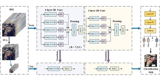
• To improve the classification accuracy of small training samples, based on DBB, MSMBB and 3D-MSMBB are proposed. In the training phase, these two modules combine the structural features of asymmetric convolution and multi-branching to explore complementary information through different sensory fields, to achieve adequate feature extraction for small-sample datasets. In the testing phase, MSMBB and 3D-MSMBB are equivalently transformed into a single convolutional layer for deployment, to reduce test resource consumption.
• To reduce the size of the network model, without significantly affecting the classification accuracy, we introduce pruning modules in the master branch of each MSMBB and 3D-MSMBB. The size of the MSMBB and 3D-MSMBB transformed convolutional layers is reduced by pruning the input channels of the pruning module, thus reducing the computational effort of the network.
• To the best of our knowledge, our method combines DBB with pruning for the first time and extends it to 3D-CNN for HSI classification. The experimental results show that the method can obtain better classification results with a smaller number of training samples and resolve the problem of low classification accuracy for small-sample datasets, as well as achieving a lightweight model.

The rest of the paper is organized as follows: Section 2 introduces the work related to the proposed method. Section 3 presents the experimental results and analysis. Section 4 describes and discusses the results. Finally, Section 5 provides the conclusion.

2. Materials and Methods

2.1. Proposed Method

The general framework of the hyperspectral image classification network based on a pruning multi-scale multi-branch hybrid convolutional network (PMBMSN) is shown in Figure 1. First, the spectral dimension of the original data is downscaled using principal component analysis (PCA) [45] to reduce the computation, while retaining the primary spectral information. After PCA, the joint spatial–spectral features of the hyperspectral images are extracted by three 3D-PMSMBBs, then the spatial features are further extracted by two PMSMBBs. Among these, the 3D-PMSMBB contains five branches and the PMSMBB contains four branches, each of which uses a different convolutional kernel size. In addition, $1\times 1\times 1$ and $1\times 1$ convolutions are added to the master branches of the 3D-PMSMBB and PMSMBB for pruning, respectively. In the test phase, each 3D-PMSMBB and PMSMBB is transformed into a corresponding single 3D or 2D convolutional layer. Finally, the above output features are input to the two fully connected layers to extract discriminative features for classification by Softmax, and the final classification results for each class are obtained.

In this paper, the original input of HSI data is represented as I ∈ R^H×W×C in the model, where $H$, $W$, and $C$ denote the height, width, and spectral dimension of the dataset, respectively. Each HSI pixel in $I$ contains $C$ spectral bands. Hyperspectral images are characterized by high dimensionality and severe redundancy. Considering the large correlation between the adjacent channels of hyperspectral images and the existence of more information redundancy, a large computational overhead will be incurred if the processing is performed directly. Therefore, to reduce spectral redundancy, most hyperspectral image classification methods first reduce the dimensions of the image to alleviate the issue of dimensionality. The dimensionality reduction methods commonly used for hyperspectral image classification include PCA [45], independent component analysis (ICA) [46], and linear discriminant analysis (LDA) [47]. Ghaffari et al. [48] recognized the essential spectral pixels by using the support of the convex hull of the principal component scores to eliminate the pixel redundancy of the dataset. Among them, PCA is the most commonly used dimensionality reduction method and is not limited by sample labels. It can reduce the dimension of the spectral bands and maintain the integrity of the spatial information. At present, it is still widely used in the dimensionality reduction processing of various hyperspectral image classification methods [49,50,51]. Therefore, PCA was used for dimensionality reduction in this study. PCA reduces the number of spectral bands from $C$ to $D,$ while keeping the spatial dimensionality unchanged. After dimensionality reduction, only the number of spectral bands is reduced in the original data and the spatial information is preserved, which is extremely important for the subsequent recognition of any object. The data cube after dimensionality reduction is denoted as $X\in R^{H\times W\times D}$, where $X$ is the input after PCA and $D$ represents the number of spectral bands after PCA. Next, the HSI data cube $X$ obtained after PCA is divided into multiple overlapping small 3D patches $O\in R^{S\times S\times D}$, where $S$ represents the height and width of $O$. The total number of small 3D patches obtained is $\left(H-S+1\right)\times \left(W-S+1\right)$, and the truth label of each small patch is determined by the label of the central pixel. These small 3D patches contain all the spectral and spatial information of $X$.

2.2. MSMBB and 3D-MSMBB

Although the various types of hybrid convolutional neural network model can extract comprehensive and deep features of hyperspectral images, these methods normally require a sufficient amount of training samples. The limited training samples of hyperspectral images limit the learning ability of deep learning models to a certain extent, making it difficult to extract typical features in hyperspectral images, which affects the classification accuracy of hyperspectral images. The multi-scale structure contains rich contextual information and has a natural advantage in hyperspectral image classification.

2.2.1. MSMBB

An MSMBB is a multi-scale multi-branch structure, in which each branch contains a convolutional kernel of different scales, to enrich the feature space of the network. In the training phase, the feature information extracted from this multi-scale multi-branch network structure is richer than that extracted from a single convolution network. In the testing phase, the multi-branch structure is re-parameterized and fused into a master branch, without using additional network parameters. The conversion process of an MSMBB is shown in Figure 2. An MSMBB contains four branches and, inspired by ACNet [52], we incorporated the idea of asymmetric convolution and designed the convolution kernels of each branch as $1\times 1$, $1\times K$, $K\times 1$, and $K\times K$, respectively. The $1\times 1$ convolution performs a linear combination of each pixel point on different channels and can preserve the original structure of the image. The two one-dimensional convolutions, $K\times 1$ and $1\times K$, enhance the square convolution kernels in horizontal and vertical directions, respectively, focusing on different local salient features from different directions. To speed up the convergence during model training and to improve the generalization ability of the network [53], we performed batch normalization (BN) after the convolution layer of each branch and combined the output of the four branches as the output of an MSMBB. The BN normalizes the feature maps of each branch, so that the output features of each branch are nonlinear, reducing the divergence of the data and effectively avoiding the occurrence of gradient explosion or gradient disappearance. In addition, the parameters of the BN are fixed in the testing phase. The multi-branch structure of the BN is introduced to solve the problem of the slow convergence of the network and to make the training process of the model more stable. The structure of the MSMBB is shown in Figure 2a.

In the testing stage, an MSMBB can be transformed into a $K\times K$ convolution, as shown in Figure 2c. The parameters of the convolution kernel of size $M\times N$ are defined as $F_{\left(M\times N\right)}\in R^{C_i\times C_o\times M\times N}$ and the bias parameters of the convolution kernel as $b\in R^{C_o}$, where $C_i$ is the number of channels of the input and $C_o$ is the number of channels of the output. To accelerate the inference process, we merge the BN layer parameters of each branch put into the convolutional layer and fuse them into one convolution, which turns the two-step operation into one step and reduces the computation and the number of parameters of the model for acceleration purposes. The BN layer includes the channel mean $\mu \in R^{C_o}$, the channel standard deviation $\sigma \in R^{C_o}$, the scaling parameter $\gamma \in R^{C_o}$, and the bias $\beta \in R^{C_o}$. $REP\left(x\right)\in R^{C_i\times C_o\times M\times N}$ denotes copying $x\in R^{C_o}$ into a matrix of the same size as $F_{\left(M\times N\right)}$. $P\left(F_{\left(M\times N\right)}\right)\in R^{C_i\times C_o\times K\times K}, M,N\le K$ denotes padding the convolution of $M\times N$ to $K\times K$. Transform1 in Figure 2 denotes transforming a convolutional layer with a convolutional kernel size of $M\times N$ and a BN layer into a convolutional layer with a convolutional kernel size of $K\times K$. The formula for Transform1 is as follows:

$$F_{\left(K\times K\right)}^{\prime }=\frac{REP\left(\gamma \right)}{REP\left(\sigma \right)}P\left(F_{\left(M\times N\right)}\right),$$

(1)

$$b^{\prime }=-\frac{\mu \gamma }{\sigma }+\beta ,$$

(2)

where $F_{\left(K\times K\right)}^{\prime }$ and $b^{\prime }$ are the converted convolution kernel weight parameter and the convolution kernel bias parameter, respectively. The convolution and BN on each branch can be converted into separate convolutions by Transform1, as shown in Figure 2b. Finally, the convolutional products of the four branches are summed, to obtain the final transformed convolutional product using the following equation:

$$F_{\left(K\times K\right)}^{″}={{\displaystyle \sum }}_{i=1}^4{F}_{i_{\left(K\times K\right)}}^{\prime },$$

(3)

$$b^{″}={{\displaystyle \sum }}_{i=1}^4{b}_i^{\prime },$$

(4)

where $F_{\left(K\times K\right)}^{″}$ and $b^{″}$ are the results of Transform2; and $F_{i_{\left(K\times K\right)}}^{\prime }$, $b_i^{\prime }$ are the convolution kernel weights and bias of the i-th branch. Combining Equations (1) and (2) yields the transformation equation of the MSMBB module, as follows:

$$F_{\left(K\times K\right)}^{″}={{\displaystyle \sum }}_{i=1}^4\frac{REP\left({\gamma }_i\right)}{REP\left({\sigma }_i\right)}P\left(F_{i_{\left(M\times N\right)}}\right),$$

(5)

$$b^{″}={{\displaystyle \sum }}_{i=1}^4-\frac{{\mu }_i{\gamma }_i}{{\sigma }_i}+{\beta }_i,$$

(6)

2.2.2. 3D-MSMBB

Conventional convolutional neural networks are generally two-dimensional and cannot extract both the spectral and spatial features of hyperspectral images, as this would destroy the correlation between pixels and thus the spectral feature information of the images. In contrast, 3D CNN can convolve in both spatial and spectral dimensions, and can adequately extract spectral–spatial features. Therefore, in this paper, we propose a 3D-DBB based on DBB and construct a 3D-MBMSB similar to MBMSB. In the 3D-MBMSB, five concurrent $1\times 1\times 1$, $1\times 1\times B$, $1\times K\times 1$, $K\times 1\times 1,$ and $K\times K\times B$ convolutions are used to replace the original $K\times K\times B$ convolution, and the BN of each branch is replaced by the BN of 3D. A 3D-MSMBB can effectively enhance the expression ability of network models. In the training stage, a 3D-MSMBB can be transformed into a 3D convolution of $K\times K\times B$. The transformation process of the 3D-MSMBB is shown in Figure 3.

Similar to the conversion formula for an MSMBB, the conversion formula of a 3D-MSMBB is as follows:

$$F_{\left(K\times K\times B\right)}^{″}={{\displaystyle \sum }}_{i=1}^5\frac{RE{P}_{3D}\left({\gamma }_i\right)}{RE{P}_{3D}\left({\sigma }_i\right)}P\left(F_{i_{\left(M\times N\times B\right)}}\right),$$

(7)

$$b^{″}={{\displaystyle \sum }}_{i=1}^5-\frac{{\mu }_i{\gamma }_i}{{\sigma }_i}+{\beta }_i,$$

(8)

where $F_{i_{\left(M\times N\times B\right)}}\in R^{C_i\times C_o\times M\times N\times B}$ represents the weight of the 3D convolution kernel on the ith branch; $B$ denotes the size of the convolution kernel on the spectral segment. $P\left(F_{\left(M\times N\times B\right)}\right)\in R^{C_i\times C_o\times K\times K\times B}, M,N,B\le K$ refers to the convolution padding of $M\times N\times B$ as $K\times K\times K$; and $RE{P}_{3D}\left(x\right)\in R^{C_i\times C_o\times M\times N\times B}$ stands for the replication of $x\in R^{C_o}$ into a matrix of the same size as $F_{\left(M\times N\times B\right)}$.

2.3. Pruning Multi-Scale Multi-Branch Block

To reduce the number of parameters of the network in the training phase, a PMSMBB combined with pruning is proposed in this paper, consisting of an MSMBB and a pruning module. Specifically, for the 3D-PMSMBB, the pruning module contains a $1\times 1\times 1$ convolution with a bias of 0. For the PMSMBB, the pruning module is the corresponding 1 × 1 convolution. The pruning module is placed on the output trunk of each multi-scale multi-branch block, and by pruning the input channels of the pruning module, the weight parameters in the multi-scale multi-branch block that have less influence on the loss can be removed in the dimension of the output. The pruning process of 3D-PMSMBB is shown in Figure 4.

The 3D-MSMBB is equivalent through transformation to a $3\times 3\times B$ convolution, whose input channel is $C_i$ and the output channel is $C_o$. The input channel and output channel of the $1\times 1\times 1$ convolution are both $C_o$. For the sake of discussion, for the 3D convolution with a convolution kernel size of $1\times 1\times 1$ and the 2D convolution with a convolution kernel size of $1\times 1$, their parameters $F_{\left(1\times 1\times 1\right)}\in R^{C_o\times C_o\times 1\times 1\times 1}$ and $F_{\left(1\times 1\right)}\in R^{C_o\times C_o\times 1\times 1}$ can both be transformed into a two-dimensional matrix $W\in R^{C_o\times C_o}$. The rows and columns of $W$ correspond to the input and output channels of the convolution, respectively, and setting a row in $W$ to zero is equivalent to pruning the input channel corresponding to the convolution. To determine the importance of each channel in $W$, this paper evaluates the importance of the parameter $w$ by estimating the effect on the loss after setting it to zero. The input to the network is $x$, the label is $y$, and the loss function is $L$. $\mathsf{\Theta }$ denotes the set of network parameters. Normally, the parameters of the network have a small range around 0. Therefore, the change in the loss $L$ after a certain parameter $w$ is set to 0 can be effectively approximated as a first-order Taylor series expansion of the loss $L$ on $w$ [43,44]. The calculation is as follows:

$$L\left(x,y,{\mathsf{\Theta }}_{w\leftarrow 0}\right)-L\left(x,y,\mathsf{\Theta }\right)=\frac{\partial L\left(x,y,\mathsf{\Theta }\right)}{\partial w}w=T\left(x,y,w\right),$$

(9)

where $T$ denotes the importance fraction of the parameter, and the larger $T$ is, the greater the impact on the loss after setting the parameter to 0 (i.e., the more important the parameter is). The importance $T_p\in R^{C_o}$ of the input channel $p$ in $W$ can be expressed as:

$$T_p=\left|{{\displaystyle \sum }}_{q=0}^{C_o}T\left(x,y,W_{p,q}\right)\right|.$$

(10)

The set of values of $T_p$ are denoted by $\Psi$ for all pruning modules in the network. As the network used in this paper has a smaller number of parameters compared with the classification network targeted by traditional pruning methods, adding regularization to all parameters will lead to underfitting the model. Therefore, unlike the traditional pruning method that adds regularization to all weights, in this paper, only the first $Q$ parameters with the smallest scores have regular loss added, while the other parameters do not have regular loss added. The parameters of the pruning module are then updated at step $t$ in the following way:

$$W\left(t+1\right)\leftarrow W\left(t\right)-\alpha \left(Z\left(t+1\right)-\eta G\left(t\right)W\left(t\right)\right),$$

(11)

$$G_{p,:}\left(t\right)=\{\begin{array}{l}1 \mathrm{if} T_p\left(t\right)< \mathrm{the} Q-\mathrm{th} \mathrm{greatest} \mathrm{value} \mathrm{in} \Psi \\ 0 \mathrm{otherwise} \end{array},$$

(12)

where $\alpha$ represents the learning rate, $\eta$ is the ordinary weight decay coefficient; $Z\left(t+1\right)$ denotes the gradient term calculated according to the optimizer and loss function; and $G\in R^{C_o\times C_o}$ represents the mask matrix for choosing whether to add regularization loss to the weights. For channels with a high importance in the weights $W\left(t\right)$, the corresponding position on the mask matrix $G$ is 0, and the regularization loss is not considered in the update. For the weights with low importance in $W\left(t\right)$, the corresponding position on the mask matrix $G$ is 1, and this is gradually reduced to 0 by the regularization loss at the update time. In the training phase, if the sum of the parameters of one of the input channels in $W\left(t\right)$ is less than a threshold $\tau$, the corresponding channel in the mask is set to zero:

$$mas{k}_p=\{\begin{array}{l}0 \mathrm{if} \left|{{\displaystyle \sum }}_{q=0}^{C_o}{W}_{p,q}\right|<\tau \\ 1 \mathrm{otherwise} \end{array}.$$

(13)

After training, the position where the mask is 0 corresponds to the channel in $W$ that needs to be pruned. $W^{\prime }\in R^{C_o^{\prime }\times C_o}$ denotes the result after $W$ is pruned. $W^{\prime }$ corresponds to the weight ${F_p}_{\left(1\times 1\times 1\right)}\in R^{C_o^{\prime }\times C_o\times 1\times 1\times 1}$ with input channel $C_o^{\prime }$, output channel $C_o$, and a convolution kernel size of $1\times 1\times 1$. In the testing phase, the convolution of $K\times K\times B$ and the convolution of $1\times 1\times 1$ are jointly transformed into a convolution of $K\times K\times B$ with the following formula for the transformation process:

$$F_{\left(K\times K\times \mathrm{B}\right)}^{\prime }=F_{\left(K\times K\times \mathrm{B}\right)}⊛TRANS\left({F_p}_{\left(1\times 1\times 1\right)}\right),$$

(14)

where $⊛$ denotes the convolution operation. As $C_o^{\prime }<C_o$, the parameters of the transformed $F_{\left(K\times K\times \mathrm{B}\right)}^{\prime }\in R^{C_i\times C_o^{\prime }\times K\times K\times B}$ are smaller than $F_{\left(K\times K\times \mathrm{B}\right)}$, thus reducing the computation in the test phase. Combining Equations (7), (8) and (14), the transformation formula of the 3D-PMSMBB can be obtained as follows:

$$F_{\left(K\times K\times B\right)}^{″}={{\displaystyle \sum }}_{i=1}^5\frac{RE{P}_{3D}\left({\gamma }_i\right)}{RE{P}_{3D}\left({\sigma }_i\right)}P\left(F_{i_{\left(M\times N\times B\right)}}\right)⊛TRANS\left(F_{\left(1\times 1\times 1\right)}\right),$$

(15)

$$b^{″}={{\displaystyle \sum }}_{i=1}^5-\frac{{\mu }_i{\gamma }_i}{{\sigma }_i}+{\beta }_i.$$

(16)

Correspondingly, the transformation equation of PMSMBB is:

$$F_{\left(K\times K\right)}^{″}={{\displaystyle \sum }}_{i=1}^4\frac{REP\left({\gamma }_i\right)}{REP\left({\sigma }_i\right)}P\left(F_{i_{\left(M\times N\right)}}\right)⊛TRANS\left(F_{\left(1\times 1\right)}\right),$$

(17)

$$b^{″}={{\displaystyle \sum }}_{i=1}^4-\frac{{\mu }_i{\gamma }_i}{{\sigma }_i}+{\beta }_i,$$

(18)

2.4. Overall Algorithm Steps

The overall process of the proposed PMSMBN is shown in Algorithm 1.

Algorithm 1. PMSMBN model

Input: HSI data $I\in R^{H\times W\times C}$$, \mathrm{pixels}=H\times W$, number of bands = $C$  Output: Classification map of the test set

1. Obtain $X\in R^{H\times W\times D}$ after PCA, $X$ is divided into multiple overlapping 3D patches, with the number $\left(H-S+1\right)\times \left(W-S+1\right)$.

2. Randomly divide the 3D patches into a training set and test set according to the proportion of training and testing.

3. For $i$ in epoch;

4.  Extract spectral–spatial features through three 3D-PMSMBBs and two PMSMBBs.

5.  Flatten the 2D feature map into a 1D feature vector.

6.  Input the 1D feature vector into two linear layers.

7.  Use softmax to classify and obtain classification results.

8.  Calculate the score of each channel of each pruning part and modify the mask according to the result.

9. Transform the training model into the test model.

10. Use the test set with the test model to obtain predicted labels.

3. Experimental Results and Analysis

3.1. Hyperspectral Dataset

In this study, three hyperspectral datasets (Indian Pines (IP), Pavia University (PU), and Salinas (SA)) were used in the experiments, to validate the effects of the model. The details of each dataset are given below.

The IP dataset was acquired using an airborne visible infrared imaging spectrometer (AVIRIS). The image size is $145\times 145$ pixels, the wavelength range is 400–2000 nm, the spatial resolution is 20 m, the number of spectral bands is 220, the noise bands are excluded, and the remaining 200 bands are used as the study object. The total number of labeled pixels in this dataset is 10,249, and there are 16 categories of labeled samples, mainly including crops, woods, and other perennial plants. Its false-color map and ground-truth map are shown in Figure 5. In this paper, 5% (518 pixels) and 95% (9731 pixels) of the IP dataset were randomly selected as the training and test sets.

The PU dataset was obtained by the German airborne reflectance optical spectral imager in Pavia City, Italy. The image size is $610\times 340$ pixels, the wavelength range is 430–860 nm, the spatial resolution is 1.3 m, and the spectral band number is 103. The total number of labeled pixels in this dataset is 42,776, and there are 9 categories of labeled samples, most of which are urban land cover, such as metal plates, roofs, and concrete pavements. Its false-color map and ground-truth map are shown in Figure 6. In this paper, 1% (426 pixels) and 99% (41,924 pixels) of the PU dataset were randomly selected as the training and test sets.

The SA dataset is an image of the Salinas Valley in California taken by the AVIRIS sensor, and has a size of 512 × 217 pixels and a spatial resolution of 3.7 m. There are 224 spectral bands, excluding 20 water absorption bands, and the remaining 204 bands were used for the study. There are 54,129 labeled pixels in the SA dataset and 16 categories of labeled samples, including crops such as cauliflower, arable land, and vineyards. Its false-color map and ground-truth map are shown in Figure 7. In this paper, 1% (543 pixels) and 99% (53,043 pixels) of the SA dataset were randomly selected as the training and test sets.

3.2. Experimental Setting

All experiments in this study were conducted on an Intel(R) Core(TM) i5-1035G1 CPU @1.7 GHz 2.19 GHz server with 128 GB of RAM and NVIDIA Tesla V100 GPU. The specific program was implemented on the Ubuntu system using the PyTorch 1.10.0 deep learning framework and Python 3.6 compiler. To verify the effectiveness of the model, three quantitative metrics, including overall accuracy (OA), average accuracy (AA), and Kappa coefficient (Kappa), were used to evaluate the performance of the model. Higher values of these metrics indicate that the model is more capable in classifying. Considering OA, AA, and Kappa together, in the experiments, the batch size was set to 32, the learning rate was set to 0.001, the pruning rate was set to 0.1, and the Adam optimizer was used to make the model converge quickly. On the IP and SA datasets, the patch size of the PMSMBN was 25 × 25 and the band was 30. On the PU dataset, the patch size was 19 × 19 and the band was 15.

3.3. Experimental Results and Analysis

To validate the effectiveness of the proposed model (PMSMBN), we compared the proposed method with some representative deep learning-based hyperspectral image classification methods, including 2D-CNN [27], 3D-CNN [30], spectral–spatial residual network (SSRN) [31], hybrid spectral CNN (HybridSN) [35], spectral–spatial attention network (SSAN) [39], and end-to-end multilevel hybrid attention network (DMCN) [41]. To ensure the fairness of the experimental results, we used the network structure with the highest accuracy in the literature and the corresponding parameters for the comparison experiments. All experiments were executed with the same hardware, and the proportions of the training and the testing samples used were identical. To ensure the rigor of the experiment, for the class with fewer than three training samples, we randomly selected three samples as the training samples for this class.

Table 1. Classification results of each method for Indian Pines.

Class	2D-CNN [27] (2015)	3D-CNN [30] (2016)	SSRN [31] (2018)	HybridSN [35] (2020)	SSAN [39] (2020)	DMCN [41] (2022)	PMSMBN
1	50.02	65.08	73.68	96.77	67.74	68.29	89.36
2	73.70	76.51	83.25	86.88	84.45	87.95	95.04
3	75.07	98.39	88.44	85.30	92.05	91.81	95.76
4	98.16	98.11	77.49	98.59	91.81	98.88	98.46
5	89.85	81.01	97.33	99.48	97.84	97.14	95.37
6	87.61	92.95	86.56	92.58	93.63	89.78	93.11
7	99.21	99.73	99.62	99.36	99.88	95.83	99.96
8	90.91	98.73	96.54	98.89	99.54	96.93	99.89
9	56.03	80.00	72.22	88.89	76.19	64.71	99.89
10	89.49	97.25	90.48	89.50	91.75	89.90	96.36
11	78.47	73.77	93.79	91.75	92.49	93.32	96.78
12	74.84	67.23	88.50	82.47	91.09	90.68	94.92
13	98.56	88.12	98.37	94.29	96.74	99.76	99.86
14	97.77	96.40	92.89	91.37	92.67	98.70	99.30
15	97.73	97.66	87.87	97.82	78.24	96.47	96.06
16	87.50	71.31	98.72	73.87	77.27	97.59	80.19
OA	83.36 ± 1.66	83.30 ± 1.63	90.29 ± 0.57	90.57 ± 0.33	91.02 ± 0.22	92.92 ± 0.54	96.28 ± 0.46
AA	84.31 ± 0.53	86.82 ± 1.55	89.13 ± 0.36	91.78 ± 0.57	89.00 ± 0.75	91.12 ± 0.61	95.67 ± 0.68
Kappa	80.88 ± 1.66	80.72 ± 1.48	88.92 ± 0.13	89.20 ± 0.58	89.75 ± 0.98	91.91 ± 0.40	95.76 ± 0.44

,

Table 2. Classification results of each method for Pavia University.

Class	2D-CNN [27] (2015)	3D-CNN [30] (2016)	SSRN [31] (2018)	HybridSN [35] (2020)	SSAN [39] (2020)	DMCN [41] (2022)	PMSMBN
1	76.65	71.47	94.53	93.82	84.74	94.63	96.09
2	94.91	92.72	94.97	98.60	97.92	99.08	99.44
3	89.88	83.80	88.61	90.08	90.20	89.11	94.75
4	87.83	98.09	98.71	95.43	95.31	98.52	98.04
5	99.35	99.66	99.39	99.92	99.89	97.77	100.00
6	98.45	95.16	98.64	99.19	98.17	99.52	99.31
7	89.00	97.24	89.26	92.28	95.19	97.68	92.51
8	67.63	72.63	78.79	83.54	88.46	93.74	92.20
9	16.35	71.73	96.69	88.05	96.42	89.68	95.98
OA	84.01 ± 0.66	87.31 ± 0.44	93.62 ± 0.46	95.59 ± 0.03	94.26 ± 0.25	97.18 ± 0.67	97.67 ± 0.72
AA	76.67 ± 0.53	87.29 ± 0.30	93.29 ± 024	93.43 ± 0.41	94.05 ± 0.45	95.53 ± 0.22	96.48 ± 0.85
Kappa	78.67 ± 0.68	82.80 ± 0.29	91.44 ± 0.44	94.13 ± 0.16	92.34 ± 0.23	96.25 ± 0.49	96.90 ± 0.33

and

Table 3. Classification results of each method for Salinas.

Class	2D-CNN [27] (2015)	3D-CNN [30] (2016)	SSRN [31] (2018)	HybridSN [35] (2020)	SSAN [39] (2020)	DMCN [41] (2022)	PMSMBN
1	99.95	99.96	100.00	100.00	100.00	100.00	100.00
2	98.23	98.90	99.43	100.00	98.84	99.92	100.00
3	98.59	97.54	100.00	99.86	99.64	100.00	100.00
4	98.15	89.88	96.93	77.97	99.17	99.85	100.00
5	96.61	98.84	98.11	99.95	97.41	99.80	98.98
6	93.80	99.51	97.82	99.70	97.21	99.84	100.00
7	98.94	99.54	99.92	99.61	99.94	99.97	99.92
8	84.75	92.79	91.15	99.49	98.93	95.78	99.90
9	91.25	99.87	99.32	99.89	99.37	99.93	100.00
10	99.47	95.66	98.55	99.16	100.00	99.94	99.91
11	96.80	89.37	99.27	97.00	99.06	99.90	100.00
12	99.66	98.71	99.84	99.14	99.57	100.00	98.85
13	81.03	75.23	95.31	98.00	99.53	97.85	99.67
14	87.25	96.41	88.32	98.44	84.16	99.61	99.62
15	87.90	99.97	98.83	98.85	99.02	99.23	99.35
16	99.64	97.76	99.72	100.00	100.00	100.00	100.00
OA	92.41 ± 0.22	95.70 ± 0.34	97.09 ± 0.33	98.19 ± 0.60	98.38 ± 0.28	98.98 ± 0.35	99.78 ± 0.19
AA	94.52 ± 0.81	95.86 ± 0.79	97.79 ± 0.58	97.26 ± 0.47	97.40 ± 0.39	99.13 ± 0.62	99.76 ± 0.13
Kappa	91.54 ± 0.53	96.33 ± 0.63	96.76 ± 0.47	97.98 ± 0.16	98.19 ± 0.44	98.88 ± 0.39	99.76 ± 0.07

represent the different classification methods in the Indian Pines, Pavia University, and Salinas datasets, with the classification results for each class. The optimal results are shown in bold.

As can be seen in Table 1, Table 2 and Table 3, the OA, AA, and Kappa of our proposed PMSMBN were generally higher than those of other methods on the three datasets. In particular, with only 1% training samples of the SA dataset, our proposed PMSMBN could still reach 99.78% OA. This indicates that the model can accurately acquire spectral–spatial features, even if a small number of training samples are selected. The classification accuracy of 2D-CNN and 3D-CNN was the lowest, and SSRN used skip connections to extract deep feature information with higher classification accuracy than 2D-CNN and 3D-CNN. Meanwhile, HybridSN based on hybrid convolution demonstrated a large improvement in classification accuracy compared with 2D-CNN and 3D-CNN using one type of convolution alone. This is due to the difficulty of extracting the joint spectral–spatial features of hyperspectral images using a single convolutional layer for small-sample classification.

Taking the IP dataset as an example, the proposed model PMSMBN in this paper improved the OA from 90.57% to 96.29% compared with HybridSN. This shows that our model is more suitable for classification in cases with a small number of samples and has a better information extraction ability due to its multi-scale and multi-branch structural features. Both SSAN and DMCN apply the attention mechanism; however, with limited training samples, the ability of the attention mechanism to fit spatial structure information is not easily exploited. Compared with DMCN, PMSMBN had a better classification effect, although there was only a small difference in the classification accuracy of DMCN compared with PMSMBN on the PU and SA datasets. The overall accuracy of the proposed model was improved by 3.36%, the average accuracy was improved by 4.55%, and the Kappa coefficient was improved by 3.85% on the IP dataset. By observing the experimental results of small-sample classification, we found that the proposed method had a better classification performance. This is because our method was designed with a multi-scale multi-branch feature extraction module, which extracts deeper spectral–spatial features by combining multiple branches of various scales and complexities, making the extracted features more comprehensive and proving the effectiveness of multi-scale multi-branch networks.

Figure 8, Figure 9 and Figure 10 show the classification results of the different models on the IP, PU, and SA datasets, along with their corresponding ground truth maps. It can be seen from the classification plots that the classification images obtained using only 2D convolution or 3D convolution had more misclassifications. The misclassifications in the classification maps obtained based on SSRN, HybridSN, SSAN, and DMCN were reduced. In particular, our proposed model showed better classification results and clearer boundaries. Comparing the classification result maps of all models with the ground-truth maps, the proposed models achieved more accurate classification results and the classification result maps were closest to the ground-truth maps.

To further evaluate the performance of the proposed model, different percentages of training samples were selected for the experiments. Of the IP dataset, 1%, 2%, 5%, 10%, and 15%, along with 0.1%, 0.2%, 0.5%, 1%, and 5% of the PU and SA datasets, were randomly selected as the training set, and the rest were used as the test set. The experimental results are shown in Figure 11. It can be seen from Figure 11 that the OA of the proposed PMSMBN model exceeded 70% when the percentage of training samples of the IP dataset was 1%. The overall accuracy of the proposed model was also significantly better when the proportion of training samples of the PU and SA datasets was 0.1%. As the number of training samples increased, each method could obtain higher classification accuracy, but the classification accuracy of the proposed method was still higher than that of the other methods. This indicates that the method can obtain good classification results with good generalization ability, both with a small number of training samples and with sufficient samples.

3.4. Ablation Analysis

To verify the validity of the multi-branch part, we replaced the multi-branch part with one branch. Specifically, three 3D-MSMBBs were replaced by three 3D-CNNs with scales of $3\times 3\times 7$, $3\times 3\times 5$, and $3\times 3\times 3$. Two MSMBBs were replaced by two 2D-CNNs with scales of $3\times 3$, and the other structures remained the same. Figure 12a shows the classification results of different training samples of the three datasets. From the figure, it can be seen that the model without 3D-MSMBBs or MSMBBs had significantly lower classification accuracy compared to the proposed PMSMBN. The advantage of the proposed model was more significant in the case of both large and small training samples. This is because our designed multi-branch structure can extract richer spectral space features using convolution kernels at different scales, which can effectively improve the classification accuracy. The experimental results demonstrated that the proposed multi-branch part can enhance the feature extraction ability of the network model.

In the same way, to verify the effectiveness of the pruning part, we tested the proposed PMSMBN and the network without the pruning part on three datasets for comparison. The experimental results are shown in Figure 12b. As can be seen from the figure, with a very small number of training samples, the difference in OA between the PMSMBN and the network without the pruning part was approximately 0.5%. As the number of samples increased, the difference in OA gradually decreased, and when the number of samples was sufficiently large, the OA of the models with and without pruning was very close. In addition, the pruned part could effectively reduce the size of the model. The pruning rate for different sample sizes is shown by the polylines in the figure, and it can be concluded from the figure that the pruned part can reduce the network model without significantly affecting the OA, achieving a lightweight model.

4. Discussion

The experimental results on the IP, PU, and SA datasets demonstrated the effectiveness of the method proposed in this paper. Compared with the other classification models, although the PMSMBN achieved better classification results on the HSI small-sample classification problem, it remained a great challenge to improve the classification performance of the model in the case of very small classification samples. Therefore, future research will focus on using open hyperspectral data to supplement small samples, combining the network model with the expanded sample approach, and thus improving the classification accuracy. In addition, the edges of each sample species of the hyperspectral images also contain rich features, and most network models have difficulty in achieving accurate recognition of edge features. Therefore, our future research direction will explore the edge feature information extraction of hyperspectral images, in combination with novel image preprocessing methods. Taking the SA dataset with the largest number of training samples as an example, the training time of the proposed model was 162.59 s and the test time was 12.93 s. On the basis of maintaining the classification accuracy of the model, we will continue to optimize the model structure, to further save training and test time.

5. Conclusions

In this paper, a pruning multi-scale multi-branch hybrid convolutional network (PMSMBN) for HSI classification was proposed. The PMSMBN addresses the problem of the the low classification accuracy of hyperspectral images with small samples and utilizes a multi-branch multi-scale block with different scales. Using MSMBB, the features of hyperspectral images can be extracted at different scales. In addition, to make the model more applicable to the characteristics of hyperspectral data redundancy, PMSMBN combines the feature that multi-branch blocks can be equivalently transformed and introduces a pruning part into the main branch of MSMBB, to reduce the number of useless parameters. We extended the idea of DBB into 3D, and proposed a 3D-PMSMBB, applying it to the field of hyperspectral image classification for the first time. To validate the effectiveness of the proposed method, we conducted a comparative experiment using the PMSMBN with other classification methods on three publicly available hyperspectral datasets. The experimental results showed that the method in this paper can more fully extract the spectral–spatial features of hyperspectral images with small training samples, and the classification accuracy was significantly better than that of other methods. For datasets with an extremely uneven sample distribution, the multi-scale multi-branch structure proposed in this paper can maintain the accuracy of the model’s performance.

References

1. Lu, Z.; Xu, B.; Sun, L.; Zhan, T.; Tang, S. 3-D Channel and Spatial Attention Based Multiscale Spatial–Spectral Residual Network for Hyperspectral Image Classification. IEEE J. Sel. Top. Appl. Earth Obs. Remote Sens. 2020, 13, 4311–4324. [Google Scholar] [CrossRef]
2. Shi, Q.; Tang, X.; Yang, T.; Liu, R.; Zhang, L. Hyperspectral Image Denoising Using a 3-D Attention Denoising Network. IEEE Trans. Geosci. Remote Sens. 2021, 59, 10348–10363. [Google Scholar] [CrossRef]
3. Tian, S.; Lu, Q.; Wei, L. Multiscale Superpixel-Based Fine Classification of Crops in the UAV-Based Hyperspectral Imagery. Remote Sens. 2022, 14, 3292. [Google Scholar] [CrossRef]
4. Yadav, C.S.; Pradhan, M.K.; Gangadharan, S.M.P.; Chaudhary, J.K.; Singh, J.; Khan, A.A.; Haq, M.A.; Alhussen, A.; Wechtaisong, C.; Imran, H.; et al. Multi-Class Pixel Certainty Active Learning Model for Classification of Land Cover Classes Using Hyperspectral Imagery. Electronics 2022, 11, 2799. [Google Scholar] [CrossRef]
5. Fang, C.; Han, Y.; Weng, F. Monitoring Asian Dust Storms from NOAA-20 CrIS Double CO2 Band Observations. Remote Sens. 2022, 14, 4659. [Google Scholar] [CrossRef]
6. Han, X.; Zhang, H.; Sun, W. Spectral Anomaly Detection Based on Dictionary Learning for Sea Surfaces. IEEE Geosci. Remote Sens. Lett. 2022, 19, 1–5. [Google Scholar] [CrossRef]
7. Wang, Z.; He, M.; Ye, Z.; Xu, K.; Nian, Y.; Huang, B. Reconstruction of Hyperspectral Images from Spectral Compressed Sensing Based on a Multitype Mixing Model. IEEE J. Sel. Top. Appl. Earth Obs. Remote Sens. 2020, 13, 2304–2320. [Google Scholar] [CrossRef]
8. Yu, C.; Han, R.; Song, M.; Liu, C.; Chang, C.-I. Feedback Attention-Based Dense CNN for Hyperspectral Image Classification. IEEE Trans. Geosci. Remote Sens. 2022, 60, 1–16. [Google Scholar] [CrossRef]
9. Melgani, F.; Bruzzone, L. Classification of Hyperspectral Remote Sensing Images with Support Vector Machines. IEEE Trans. Geosci. Remote Sens. 2004, 42, 1778–1790. [Google Scholar] [CrossRef] [Green Version]
10. Ma, L.; Crawford, M.M.; Tian, J. Local Manifold Learning-Based k-Nearest-Neighbor for Hyperspectral Image Classification. IEEE Trans. Geosci. Remote Sens. 2010, 48, 4099–4109. [Google Scholar] [CrossRef]
11. Li, J.; Bioucas-Dias, J.M.; Plaza, A. Spectral–Spatial Hyperspectral Image Segmentation Using Subspace Multinomial Logistic Regression and Markov Random Fields. IEEE Trans. Geosci. Remote Sens. 2012, 50, 809–823. [Google Scholar] [CrossRef]
12. Qian, Y.; Ye, M.; Zhou, J. Hyperspectral Image Classification Based on Structured Sparse Logistic Regression and Three-Dimensional Wavelet Texture Features. IEEE Trans. Geosci. Remote Sens. 2013, 51, 2276–2291. [Google Scholar] [CrossRef] [Green Version]
13. Zhu, Z.; Jia, S.; He, S.; Sun, Y.; Ji, Z.; Shen, L. Three-Dimensional Gabor Feature Extraction for Hyperspectral Imagery Classification Using a Memetic Framework. Inf. Sci. 2015, 298, 274–287. [Google Scholar] [CrossRef]
14. Dundar, T.; Ince, T. Sparse Representation-Based Hyperspectral Image Classification Using Multiscale Superpixels and Guided Filter. IEEE Geosci. Remote Sens. Lett. 2019, 16, 246–250. [Google Scholar] [CrossRef]
15. Duan, P.; Kang, X.; Li, S.; Ghamisi, P.; Benediktsson, J.A. Fusion of Multiple Edge-Preserving Operations for Hyperspectral Image Classification. IEEE Trans. Geosci. Remote Sens. 2019, 57, 10336–10349. [Google Scholar] [CrossRef]
16. Chen, Y.; Lin, Z.; Zhao, X.; Wang, G.; Gu, Y. Deep Learning-Based Classification of Hyperspectral Data. IEEE J. Sel. Top. Appl. Earth Obs. Remote Sens. 2014, 7, 2094–2107. [Google Scholar] [CrossRef]
17. Chen, Y.; Zhao, X.; Jia, X. Spectral–Spatial Classification of Hyperspectral Data Based on Deep Belief Network. IEEE J. Sel. Top. Appl. Earth Obs. Remote Sens. 2015, 8, 2381–2392. [Google Scholar] [CrossRef]
18. Mou, L.; Ghamisi, P.; Zhu, X.X. Deep Recurrent Neural Networks for Hyperspectral Image Classification. IEEE Trans. Geosci. Remote Sens. 2017, 55, 3639–3655. [Google Scholar] [CrossRef] [Green Version]
19. Li, Y.; Zhang, H.; Shen, Q. Spectral–Spatial Classification of Hyperspectral Imagery with 3D Convolutional Neural Network. Remote Sens. 2017, 9, 67. [Google Scholar] [CrossRef] [Green Version]
20. Hong, D.; Gao, L.; Yao, J.; Zhang, B.; Plaza, A.; Chanussot, J. Graph Convolutional Networks for Hyperspectral Image Classification. IEEE Trans. Geosci. Remote Sens. 2021, 59, 5966–5978. [Google Scholar] [CrossRef]
21. Zhang, X.; Sun, G.; Jia, X.; Wu, L.; Zhang, A.; Ren, J.; Fu, H.; Yao, Y. Spectral–Spatial Self-Attention Networks for Hyperspectral Image Classification. IEEE Trans. Geosci. Remote Sens. 2022, 60, 1–15. [Google Scholar] [CrossRef]
22. Zheng, J.; Feng, Y.; Bai, C.; Zhang, J. Hyperspectral Image Classification Using Mixed Convolutions and Covariance Pooling. IEEE Trans. Geosci. Remote Sens. 2021, 59, 522–534. [Google Scholar] [CrossRef]
23. Wang, W.; Chen, Y.; He, X.; Li, Z. Soft Augmentation-Based Siamese CNN for Hyperspectral Image Classification with Limited Training Samples. IEEE Geosci. Remote Sens. Lett. 2022, 19, 1–5. [Google Scholar] [CrossRef]
24. Wu, X.; Hong, D.; Chanussot, J. Convolutional Neural Networks for Multimodal Remote Sensing Data Classification. IEEE Trans. Geosci. Remote Sens. 2022, 60, 1–10. [Google Scholar] [CrossRef]
25. Sultana, F.; Sufian, A.; Dutta, P. Evolution of Image Segmentation Using Deep Convolutional Neural Network: A Survey. Knowl. -Based Syst. 2020, 201–202, 106062. [Google Scholar] [CrossRef]
26. Hu, W.; Huang, Y.; Wei, L.; Zhang, F.; Li, H. Deep Convolutional Neural Networks for Hyperspectral Image Classification. J. Sens. 2015, 2015, e258619. [Google Scholar] [CrossRef] [Green Version]
27. Makantasis, K.; Karantzalos, K.; Doulamis, A.; Doulamis, N. Deep Supervised Learning for Hyperspectral Data Classification through Convolutional Neural Networks. In Proceedings of the 2015 IEEE International Geoscience and Remote Sensing Symposium (IGARSS), Milan, Italy, 26–31 July 2015; pp. 4959–4962. [Google Scholar]
28. Fang, L.; Liu, Z.; Song, W. Deep Hashing Neural Networks for Hyperspectral Image Feature Extraction. IEEE Geosci. Remote Sens. Lett. 2019, 16, 1412–1416. [Google Scholar] [CrossRef]
29. Li, W.; Wu, G.; Zhang, F.; Du, Q. Hyperspectral Image Classification Using Deep Pixel-Pair Features. IEEE Trans. Geosci. Remote Sens. 2017, 55, 844–853. [Google Scholar] [CrossRef]
30. Chen, Y.; Jiang, H.; Li, C.; Jia, X.; Ghamisi, P. Deep Feature Extraction and Classification of Hyperspectral Images Based on Convolutional Neural Networks. IEEE Trans. Geosci. Remote Sens. 2016, 54, 6232–6251. [Google Scholar] [CrossRef] [Green Version]
31. Zhong, Z.; Li, J.; Luo, Z.; Chapman, M. Spectral–Spatial Residual Network for Hyperspectral Image Classification: A 3-D Deep Learning Framework. IEEE Trans. Geosci. Remote Sens. 2018, 56, 847–858. [Google Scholar] [CrossRef]
32. Wang, W.; Dou, S.; Jiang, Z.; Sun, L. A Fast Dense Spectral–Spatial Convolution Network Framework for Hyperspectral Images Classification. Remote Sens. 2018, 10, 1068. [Google Scholar] [CrossRef] [Green Version]
33. Paoletti, M.E.; Haut, J.M.; Fernandez-Beltran, R.; Plaza, J.; Plaza, A.; Li, J.; Pla, F. Capsule Networks for Hyperspectral Image Classification. IEEE Trans. Geosci. Remote Sens. 2019, 57, 2145–2160. [Google Scholar] [CrossRef]
34. Tinega, H.C.; Chen, E.; Ma, L.; Nyasaka, D.O.; Mariita, R.M. HybridGBN-SR: A Deep 3D/2D Genome Graph-Based Network for Hyperspectral Image Classification. Remote Sens. 2022, 14, 1332. [Google Scholar] [CrossRef]
35. Roy, S.K.; Krishna, G.; Dubey, S.R.; Chaudhuri, B.B. HybridSN: Exploring 3-D–2-D CNN Feature Hierarchy for Hyperspectral Image Classification. IEEE Geosci. Remote Sens. Lett. 2020, 17, 277–281. [Google Scholar] [CrossRef] [Green Version]
36. Zhu, M.; Jiao, L.; Liu, F.; Yang, S.; Wang, J. Residual Spectral–Spatial Attention Network for Hyperspectral Image Classification. IEEE Trans. Geosci. Remote Sens. 2021, 59, 449–462. [Google Scholar] [CrossRef]
37. Wu, H.; Li, D.; Wang, Y.; Li, X.; Kong, F.; Wang, Q. Hyperspectral Image Classification Based on Two-Branch Spectral–Spatial-Feature Attention Network. Remote Sens. 2021, 13, 4262. [Google Scholar] [CrossRef]
38. Hang, R.; Li, Z.; Liu, Q.; Ghamisi, P.; Bhattacharyya, S.S. Hyperspectral Image Classification with Attention-Aided CNNs. IEEE Trans. Geosci. Remote Sens. 2021, 59, 2281–2293. [Google Scholar] [CrossRef]
39. Sun, H.; Zheng, X.; Lu, X.; Wu, S. Spectral–Spatial Attention Network for Hyperspectral Image Classification. IEEE Trans. Geosci. Remote Sens. 2020, 58, 3232–3245. [Google Scholar] [CrossRef]
40. Dong, Z.; Cai, Y.; Cai, Z.; Liu, X.; Yang, Z.; Zhuge, M. Cooperative Spectral–Spatial Attention Dense Network for Hyperspectral Image Classification. IEEE Geosci. Remote Sens. Lett. 2021, 18, 866–870. [Google Scholar] [CrossRef]
41. Xiang, J.; Wei, C.; Wang, M.; Teng, L. End-to-End Multilevel Hybrid Attention Framework for Hyperspectral Image Classification. IEEE Geosci. Remote Sens. Lett. 2022, 19, 1–5. [Google Scholar] [CrossRef]
42. Ding, X.; Zhang, X.; Han, J.; Ding, G. Diverse Branch Block: Building a Convolution as an Inception-like Unit. In Proceedings of the 2021 IEEE/CVF Conference on Computer Vision and Pattern Recognition (CVPR), Nashville, TN, USA, 20–25 June 2021; pp. 10881–10890. [Google Scholar]
43. Ding, X.; Hao, T.; Tan, J.; Liu, J.; Han, J.; Guo, Y.; Ding, G. ResRep: Lossless CNN Pruning via Decoupling Remembering and Forgetting. In Proceedings of the 2021 IEEE/CVF International Conference on Computer Vision (ICCV), Montreal, QC, Canada, 10–17 October 2021; pp. 4490–4500. [Google Scholar]
44. Ding, X.; Ding, G.; Zhou, X.; Guo, Y.; Han, J.; Liu, J. Global Sparse Momentum SGD for Pruning Very Deep Neural Networks. Adv. Neural Inf. Process. Syst. 2019, 32. [Google Scholar] [CrossRef]
45. Licciardi, G.; Marpu, P.R.; Chanussot, J.; Benediktsson, J.A. Linear Versus Nonlinear PCA for the Classification of Hyperspectral Data Based on the Extended Morphological Profiles. IEEE Geosci. Remote Sens. Lett. 2012, 9, 447–451. [Google Scholar] [CrossRef] [Green Version]
46. Villa, A.; Benediktsson, J.A.; Chanussot, J.; Jutten, C. Hyperspectral Image Classification with Independent Component Discriminant Analysis. IEEE Trans. Geosci. Remote Sens. 2011, 49, 4865–4876. [Google Scholar] [CrossRef] [Green Version]
47. Bandos, T.V.; Bruzzone, L.; Camps-Valls, G. Classification of Hyperspectral Images with Regularized Linear Discriminant Analysis. IEEE Trans. Geosci. Remote Sens. 2009, 47, 862–873. [Google Scholar] [CrossRef]
48. Ghaffari, M.; Omidikia, N.; Ruckebusch, C. Essential Spectral Pixels for Multivariate Curve Resolution of Chemical Images. Anal. Chem. 2019, 91, 10943–10948. [Google Scholar] [CrossRef] [Green Version]
49. Sun, L.; Zhao, G.; Zheng, Y.; Wu, Z. Spectral–Spatial Feature Tokenization Transformer for Hyperspectral Image Classification. IEEE Trans. Geosci. Remote Sens. 2022, 60, 1–14. [Google Scholar] [CrossRef]
50. Liu, J.; Zhang, K.; Wu, S.; Shi, H.; Zhao, Y.; Sun, Y.; Zhuang, H.; Fu, E. An Investigation of a Multidimensional CNN Combined with an Attention Mechanism Model to Resolve Small-Sample Problems in Hyperspectral Image Classification. Remote Sens. 2022, 14, 785. [Google Scholar] [CrossRef]
51. Feng, Y.; Zheng, J.; Qin, M.; Bai, C.; Zhang, J. 3D Octave and 2D Vanilla Mixed Convolutional Neural Network for Hyperspectral Image Classification with Limited Samples. Remote Sens. 2021, 13, 4407. [Google Scholar] [CrossRef]
52. Ding, X.; Guo, Y.; Ding, G.; Han, J. ACNet: Strengthening the Kernel Skeletons for Powerful CNN via Asymmetric Convolution Blocks. In Proceedings of the 2019 IEEE/CVF International Conference on Computer Vision (ICCV), Seoul, Republic of Korea, 27 October–2 November 2019; pp. 1911–1920. [Google Scholar]
53. Ioffe, S.; Szegedy, C. Batch Normalization: Accelerating Deep Network Training by Reducing Internal Covariate Shift. In Proceedings of the 32nd International Conference on International Conference on Machine Learning, Lille, France, 6–11 July 2015; Volume 37, pp. 448–456. [Google Scholar]
Figure 1. The overall architecture of the proposed pruning multi-scale multi-branch hybrid convolutional network (PMSMBN) for hyperspectral image (HSI) classification: (a) training and test structure of pruning multi-scale multi-branch block (PMSMBB); (b) training and test structure of 3D-PMSMBB.
Electronics 12 00674 g001
Figure 2. The conversion process of the multi-scale multi-branch block (MSMBB): (a) MSMBB; (b) structure of MSMBB after Transform1; (c) structure of MSMBB after Transform2.
Electronics 12 00674 g002
Figure 3. The conversion process of the 3D-MBMSB: (a) 3D-MBMSB; (b) structure of 3D-MSMBB after Transform1; (c) structure of 3D-MSMBB after Transform2.
Electronics 12 00674 g003
Figure 4. The 3D-PMSMBB pruning process.
Electronics 12 00674 g004
Figure 5. Indian Pines dataset: (a) false-color map (band 29, 19, 9); (b) ground-truth map.
Electronics 12 00674 g005
Figure 6. Pavia University dataset: (a) false-color map (band 21, 41, 61); (b) ground-truth map.
Electronics 12 00674 g006
Figure 7. Salinas dataset: (a) false-color map (band 41, 21, 21); (b) ground-truth map.
Electronics 12 00674 g007
Figure 8. Classification maps of the different models for the Indian Pines dataset: (a) ground-truth image; (b) 2D-CNN; (c) 3D-CNN; (d) SSRN; (e) HybridSN; (f) SSAN; (g) DMCN; (h) proposed PMSMBN.
Electronics 12 00674 g008
Figure 9. Classification maps of the different models for the Pavia University dataset: (a) ground-truth image; (b) 2D-CNN; (c) 3D-CNN; (d) SSRN; (e) HybridSN; (f) SSAN; (g) DMCN; (h) proposed PMSMBN.
Electronics 12 00674 g009
Figure 10. Classification maps of the different models for the Salinas dataset: (a) ground-truth image; (b) 2D-CNN; (c) 3D-CNN; (d) SSRN; (e) HybridSN; (f) SSAN; (g) DMCN; (h) proposed PMSMBN.
Electronics 12 00674 g010aElectronics 12 00674 g010b
Figure 11. Varying training percent for: (a) IP dataset; (b) PU dataset; (c) SA dataset.
Electronics 12 00674 g011
Figure 12. Ablation experiments of the proposed method on three datasets. (a) without 3D-MSMBBs or MSMBBs; (b) without a pruning part.
Electronics 12 00674 g012