Introducing the UWF-ZeekDataFall22 Dataset to Classify Attack Tactics from Zeek Conn Logs Using Spark’s Machine Learning in a Big Data Framework

Abstract

This study introduces UWF-ZeekDataFall22, a newly created dataset labeled using the MITRE ATT&CK framework. Although the focus of this research is on classifying the never-before classified resource development tactic, the reconnaissance and discovery tactics were also classified. The results were also compared to a similarly created dataset, UWF-ZeekData22, created in 2022. Both of these datasets, UWF-ZeekDataFall22 and UWF-ZeekData22, created using Zeek Conn logs, were stored in a Big Data Framework, Hadoop. For machine learning classification, Apache Spark was used in the Big Data Framework. To summarize, the uniqueness of this work is its focus on classifying attack tactics. For UWF-ZeekdataFall22, the binary as well as the multinomial classifier results were compared, and overall, the results of the binary classifier were better than the multinomial classifier. In the binary classification, the tree-based classifiers performed better than the other classifiers, although the decision tree and random forest algorithms performed almost equally well in the multinomial classification too. Taking training time into consideration, decision trees can be considered the most efficient classifier.

1. Introduction

Due to the remarkable advancements in technology and increase in the number of internet users in recent times, there has been an unprecedented surge in the amount of data generated and exchanged over the internet. Millions of financial transactions are being conducted on the internet and cloud-based systems store a plethora of sensitive data, including personal, health, and other sensitive data. Given the ever-increasing magnitude of data collected and utilized, ensuring robust security measures and safeguarding against unauthorized network intrusions have become equally imperative. Also, due to the rise in network attacks, it has become very important to detect intrusions (attacks) before they happen rather than after they happen. Therefore, in order to develop stronger network intrusion systems that detect attacks before they happen, it is important to understand what an adversary is planning and how the adversary is planning to attack. The MITRE Adversarial Tactics, Techniques, and Common Knowledge (ATT&CK) framework defines tactics as being the motives of the adversary. The MITRE ATT&CK framework, which is a foundation of threat models and methodologies, is based on 14 tactics and several techniques belonging to more than one tactic [1]. Hence, data labeled as per the MITRE ATT&CK framework help us study the various tactics of the adversary. This research classifies the data that lead up to three adversary tactics, defined and labeled as per the MITRE ATT&CK framework: reconnaissance (TA0043) [2], discovery (TA0007) [3], and resource development (TA0042) [4]. A reconnaissance tactic is a phase in which an adversary attempts to gather information about a target in order to attack it [2]. A discovery tactic is a phase in which an adversary attempts to discover the target’s system resources and vulnerabilities [3]. Resource development tactics are when an adversary uses techniques to compromise resources like infrastructure, accounts, or other capabilities that can be used to support targeting [4]. Although there has been some classification work on the reconnaissance and discovery tactics [1], there has been no classification work as of yet on the resource development tactic.

This research classifies these tactics using two different datasets, UWF-ZeekData22 [5], created in 2022, and UWF-ZeekDataFall22 [5], created in 2023, both created using Zeek Conn logs. Due to the amounts of data involved, both datasets are stored in a Big Data framework, Hadoop, which is a distributed file system (Hadoop Distributed File System, HDFS). The HDFS is a scalable fault-tolerant system that allows the storage and processing of Big Data across a cluster of computers [6]. For machine learning (ML) classification, Apache Spark, an open-source computing framework that sits on top of Hadoop, is used. Spark is an in-memory cluster computing framework for processing and analyzing large amounts of data. Key features of Spark are that it is fast, scalable, and fault tolerant [7]. For the classification and comparative analysis of the performance of these two datasets, several machine learning (ML) libraries of Apache Spark are used in this work.

To summarize, the uniqueness of this work is its focus on classifying tactics rather than attacks. This work focuses on classifying the resource development tactic of the MITRE ATT&CK framework; the resource development tactic has not been previously analyzed or classified. Second, this classification is performed on a newly created dataset, UWF-ZeekDataFall22, uniquely created using Zeek and an open-source traffic analyzer [8] and labeled using the MITRE ATT&CK framework. To optimize the workings of Spark, this study also looks at the effect of the executor count, executor core count, total executor cores, executor memory, and total executor memory allocations of Spark. Furthermore, in addition to classifying the tactics of UWF-ZeekDataFall22, this study also compares the results with a similarly created dataset, UWF-ZeekData22.

This paper is organized as follows: Section 2 covers related work; Section 3 explains the data used in this work; Section 4 describes the experimentation, that is, everything from the binning to calculating the information gain; Section 5 presents the machine learning algorithms used in this work; and Section 6 presents the results. Section 7 presents a summary of the key finding and Section 8 presents the conclusions.

2. Related Work

Many experiments have been carried out in the cybersecurity field to determine the best classifier for detecting network attacks. Mebawondu et al. (2022) [9] compared the effectiveness of naïve Bayes with the C4.5 decision tree algorithm using the UNSW-NB15 dataset. In this work, the data pre-processing stage employed min–max normalization to ensure that feature values fell inside a predetermined range. They also used information gain and gain ratio algorithms to extract relevant features. In this work, the decision tree algorithm was found to perform better than naïve Bayes.

Panda and Patra (2007) [10] used the KDD’99 dataset, a subset of the DARPA dataset. Only 10% of the dataset was used in their experiment, and naïve Bayes was used for classification. The final results were compared to backpropagation neural network (BPN) results for the same dataset. Naïve Bayes was, surprisingly, found to have a higher detection rate and took less time than the BPN, but it produced more false positives.

Tufail et al. (2022) [11] compared the performance of shallow neural networks (SNN) and logistic regression in predicting DDoS assaults. They used “Divide and Randomized Conquer” to create datasets of 100 k and 1000 k packets from their initial raw dataset, which had approximately 12 million packets and 84 characteristics. It was found that the accuracy of logistic regression was slightly lower than the accuracy of SNN; however, the training time for SNN was longer than that for logistic regression.

In another study by Kejriwal et al. (2022) [12], the intrusion detection accuracy of different algorithms like logistic regression, random forest, KNN, XGBoost, Gaussian naïve Bayes, and a multi-layer perceptron classifier (MLP) were compared. The dataset used in their study was CIC-IDS2017. Of all the ML algorithms, the random forest algorithm was found to have the best results. Logistic regression was found to perform better than naïve Bayes, which had the lowest performance of all.

In yet another comparative study, Disha and Waheed (2021) [13] used the GBT classifier for binary classification to determine network intrusions using the UNSW-NB15 dataset. A Chi-squared test was used to remove irrelevant features, and GBT was discovered to have the highest accuracy after decision trees.

In Swamy et al. (2012) [14], the decision tree (DT) classifier and min–max normalization algorithms were used as part of the intrusion-detection process using the KDDP99 dataset. The DT classifier had good accuracy, with lower false positive and true negative rates.

In another study, Mulay et al. (2010) [15] compared the performance of the decision tree classifier with support vector machines (SVMs). The accuracy of decision trees was found to be high, and their training and testing times were low compared to SVMs.

Jha and Ragha (2013) [16] used the SVM classifier on the NSL-KDD dataset, which consists of selected records from the KDD99 dataset. The information gain algorithm was used in their study to extract relevant features. It was found that the reduced dataset increased the detection rate of the SVM and also reduced the training and testing times.

Belouch et al. (2018) [17] compared four well-known classification algorithms, SVM, naïve Bayes, decision tree, and random forest, using Apache Spark with the UNSW-NB15 dataset. They found that random forest gave the best performance followed by decision tree and naïve Bayes.

All the above works performed classification on network attacks. There are no works on the classification of tactics, which is the novelty of our work. Moreover, none of the above works performed classification on tactics using the two new uniquely created datasets, UWF-ZeekData22 and UWF-ZeekDataFall22.

3. The Datasets

The Zeek Conn log MITRE ATT&CK framework labeled datasets, UWF-ZeekData22 and UWF-ZeekDataFall22, available in [5], generated using the Cyber Range at the University of West Florida (UWF), were used for this analysis. UWF-ZeekData22, created in 2022, had 9,280,869 attack records and 9,281,599 benign records [18], and a breakdown of this dataset’s tactics is also presented in Bagui et al. (2023) [18]. The new dataset, UWF-ZeekDataFall22, created in 2023, has 350,001 attack records and 350,339 benign records [5]. The breakdown of the attack tactics in the UWF-ZeekDataFall22 dataset is presented in

Table 1. UWF-ZeekDataFall22 MITRE ATT&CK tactic counts.

Tactic	Count
None	350,339
Resource Development	275,471
Reconnaissance	51,492
Discovery	16,819
Privilege Escalation	3066
Defense Evasion	3064
Execution	30
Initial Access	19
Command and Control	17
Lateral Movement	11
Persistence	10
Collection	1
Credential Access	1

.

3.1. Tactics in the UWF-ZeekDataFall22 Dataset

This dataset had the highest number of resource development tactics followed by reconnaissance and discovery; hence, in this work, we focus on these three tactics.

The resource development tactic encompasses multiple techniques, with a focus on obtaining resources to help support targeting. These techniques range from creating, purchasing, or illicitly obtaining resources to including, but not limited to, infrastructure, accounts, or capabilities [4].

The reconnaissance tactic involves various techniques that are conducted to facilitate both active and passive information gathering for target development. Techniques of reconnaissance could involve trying to identify potential attack surfaces and entry points by scanning ports, mapping the topology of the network, and researching the target’s online digital footprint [2].

The discovery tactic involves various directed techniques meant to determine network infrastructure details like identifying the exact services and versions running on remote hosts or collecting technical details about the local network architecture. Going beyond the reconnaissance tactic, the discovery tactic is set on gathering precise information about the target that can be used to plan and execute specific attacks. It allows attackers or security professionals to identify vulnerabilities, misconfigurations, and targets that can be exploited [2].

3.2. The Zeek Conn Log Files of the UWF-ZeekDataFall22 Dataset

The Zeek Conn log files of the UWF-ZeekDataFall22 dataset were used in this work. The Zeek Conn log files, explained in [5,19], track the protocols and associated information such as IP addresses, duration, two-way bytes, states, packets, and tunnel information. In short, the Conn log files provide all the data regarding the connection between two points. The full list of the attributes of the Conn log files is available in [5,19]. The “mitre_attack” attribute was added to label the data.

4. Experimentation

The datasets, stored in parquet format on HDFS, were read into Spark’s data frame for processing. Spark’s data frame, organized in the form of rows and columns, allows for the easier processing of large amounts of data.

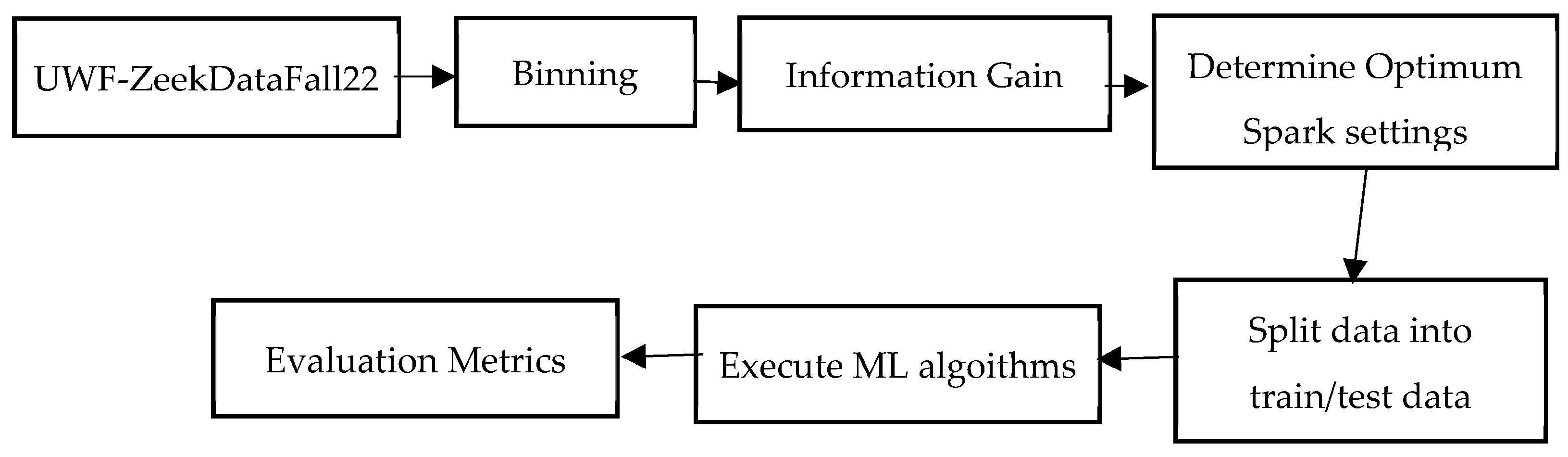
4.1. Overview of Processing UWF-ZeekDataFall22

First, the input dataset, UWF-ZeekDataFall22, was binned. Since this dataset has several continuous attributes, these attributes were binned to smoothen the data and remove noise. Also, binning was used to prepare the data for algorithms that require discrete values, like decision trees and random forest algorithms as well as gradient-boosting trees. Binning also helps to address any over-fitting issue [20].

Figure 1 presents the overview of the experimentation. As presented in Figure 1, the binned data were then used to calculate information gain. Information gain was used to determine the relevance of the features or attributes. Machine learning (ML) using Spark was performed on this preprocessed dataset, and Spark’s optimum parameters were determined before ML was used. For the ML algorithms, the input dataset was divided into training and testing sets with a ratio of 80:20. Apache Spark’s machine learning libraries for naïve Bayes, logistic regression, random forest, gradient-boosting trees, support vector machines, and decision trees were used to train and detect the network tactics. To assess the effectiveness of the machine learning classifiers, various evaluation metrics, such as accuracy, precision, and recall, were utilized for comparison.

4.2. Preprocessing Using Binning

From the Zeek Conn log files of the UWF-ZeekDataFall22 dataset, the following features were binned:

• dest_ip and src_ip for IP addresses;
• dest_port and src_port for port numbers;
• local_orig and local_resp, which are Boolean data types;
• protocol, conn_state, history, and service, all of which are nominal attributes;
• duration, orig_bytes, orig_pkts, orig_ip_bytes, resp_bytes, resp_pkts, resp_ip_bytes, and missed_bytes, which are all continuous valued attributes.

4.2.1. Binning IP Addresses

For binning the IP addresses, the commonly recognized network classifications [21] of A, B, C, D, and E were used, each of which pertains to specific ranges of the first octet in the IP address. Null and non-applicable values are assigned a value of 0, 0–127 octet values are assigned a value of 1, and so on.

Table 2. Binning IP addresses in the UWF-ZeekDataFall22 dataset.

Classification	Octet Values	Bin Number	dest_ip Count	src_ip Count
Non-class	Null or NA	0	0	0
Class A	0–127	1	3,072,966	6
Class B	<=191	2	608,348	3,719,960
Class C	<=223	3	33,482	0
Class D	<=239	4	5168	0
Class E	<=254	5	0	0
Other	If none of the above	6	2	0

presents the classification after binning the IP addresses.

4.2.2. Binning Port Numbers

Port numbers were binned following the Internet Assigned Numbers Authority (IANA) [22], administering ports 0 through 65,535. Binning was performed as per well-known ports, registered ports, and dynamic/private ports, as shown in

Table 3. Binning port numbers in the UWF-ZeekDataFall22 dataset.

Classification	Port Numbers	Bin Number	dest_port Count	src_port Count
Well-known ports	0–1023	1	3,505,385	73,900
Registered ports	<=49,151	2	205,615	2,095,923
Dynamic/private ports	<=65,535	3	65,812	1,606,989
Other	If none of the above	4	0	0

. Table 3 presents the binning of port numbers in UWF-ZeekDataFall22.

4.2.3. Binning Booleans and Nominal Attributes

Booleans and nominal values are the non-numeric data in the dataset. The StringIndexer method from MLib [23], which is Apache Spark’s scalable machine learning library, was used to convert the non-numeric values into numbers. This method also converts the invalid or null values to integer values for binning. The columns binned using this algorithm were local_orig, local_resp, protocol, conn_state, history, and service, as presented in

Table 4. Bins generated for Boolean and nominal attributes for the UWF-ZeekDataFall22 dataset.

Attributes	Count of Integer Bins
local_orig	1
local_resp	1
Protocol	2
conn_state	9
history	32
service	11

. Table 4 shows the number of bins generated for each specific attribute.

4.2.4. Binning Continuous Valued Attributes

Continuous values were binned as per [19]. Null values were dropped from the columns and then a 10% trim was performed from both ends. The trimmed version was used to calculate the mean and standard deviation, and the edges of the bins were generated as per the Algorithm 1, adopted from [19]:

Algorithm 1 Binning Continuous Valued Attributes

if min_val >= 0:

while mean_val − 2 * stddev_val < 0:

mean_val += stddev_val

edge0 = float(‘-inf’)

edge1 = mean_val − stddev_val * 2

edge2 = mean_val − stddev_val

edge3 = mean_val

edge4 = mean_val + stddev_val

edge5 = mean_val + stddev_val * 2

edge6 = float(‘inf’)

edges = [edge0, edge1, edge2, edge3, edge4, edge5, edge6]

edges_distinct = []

The Bucketizer function in Pyspark was used to generate bins using the edges. To maintain the desired number of bins and to avoid redundant bin ranges, the moving-mean logic, presented in Algorithm 2, was inserted during the establishment of the edges, adopted as per [19]:

Algorithm 2 Moving-mean Logic

if min_val >= 0:

while mean_val – 2 * stddev_val < 0:

mean_val += stddev_val

The numbers of bins generated for all continuous valued attributes are presented in

Table 5. Number of bins for continuous valued attributes in the UWF-ZeekDataFall22 dataset.

Attributes	Count of Integer Bins
duration	6
orig_bytes	6
orig_pkts	2
orig_ip_bytes	6
resp_bytes	2
resp_pkts	2
resp_ip_bytes	2
missed_bytes	2

.

4.3. Information Gain

After the binning process was completed, information gain was used to assess the relevance of each of the 18 features from the Zeek Conn Log files of the UWF-ZeekDataFall22 dataset using the binned data. The information gain algorithm was used to extract the relevant attributes.

Information gain is the difference between a class’s entropy and the entropy of the class and a selected feature split, with entropy measuring the extent of randomness in the dataset [24]. It is an assessment of the usefulness of a feature in the classification.

The following calculations [24] were performed on each attribute to produce information gain values for ranking purposes:

$$Gain\left(A\right)=Info\left(D\right)-{Info}_A\left(D\right)$$

(1)

where

$$Info\left(D\right)=-\sum _{i=1}^m{p}_i{log}_2\left(pi\right)$$

(2)

$${Info}_A\left(D\right)=\sum _{j=1}^V\frac{\left|D_j\right|}{\left|D\right|}\times Info\left(D_j\right)$$

(3)

where

• Info(D) is the average amount of information needed to identify the class level of a tuple in D;
• Info_A(D) is the expected information required to classify a tuple from D based on the partitioning from A;
• p_i is the non-zero probability that an arbitrary tuple belongs to a class;
• |D_j|/|D| is the weight of the partition.

Information gain was calculated for the full dataset and the three tactics, resource development, discovery, and reconnaissance, individually. The information gain values for the attributes in the Zeek Conn logs using the full dataset are presented in

Table 6. Information gain values for the full dataset, UWF-ZeekDataFall22.

Full Dataset
Attribute	Info_Gain
history	0.3769642
protocol	0.36886144
dest_port	0.34085092
service	0.3125681
orig_bytes	0.29707623
duration	0.29682565
resp_bytes	0.29655516
orig_ip_bytes	0.29552263
orig_pkts	0.29124352
dest_ip	0.20953701
local_resp	0.19356702
conn_state	0.022014592
src_port	0.003268247
src_ip	0.001607323
local_orig	5.02 × 10−4
missed_bytes	0
resp_ip_bytes	0
resp_pkts	0

, and for resource development, discovery, and reconnaissance in

Table 7. UWF-ZeekDataFall22: Information gain values for resource development.

Resource Development
Attribute	Info_Gain
history	0.8810788
protocol	0.8810783
dest_port	0.8239399
orig_ip_bytes	0.823516
service	0.81280994
orig_bytes	0.7881991
duration	0.7871984
resp_bytes	0.7861375
orig_pkts	0.778875
dest_ip	0.6267121
local_resp	0.59013766
conn_state	0.032609735
src_port	0.010610466
src_ip	0.005892113
local_orig	0.001804289
missed_bytes	0
resp_ip_bytes	0
resp_pkts	0

,

Table 8. UWF-ZeekDataFall22: Information gain values for discovery.

Discovery
Attribute	Info_Gain
history	0.88164663
protocol	0.8805963
conn_state	0.8794843
orig_ip_bytes	0.8471305
service	0.7876045
orig_bytes	0.7738234
duration	0.773805
resp_bytes	0.7718542
orig_pkts	0.76303893
dest_ip	0.623519
dest_port	0.60750306
local_resp	0.57914233
src_port	0.19649306
src_ip	0.00906063
local_orig	0.0017338
missed_bytes	0
resp_ip_bytes	0
resp_pkts	0

, and

Table 9. UWF-ZeekDataFall22: Information gain values for reconnaissance.

Reconnaissance
Attribute	Info_Gain
protocol	0.8821778
history	0.8709951
conn_state	0.8681412
orig_ip_bytes	0.82774657
service	0.8121441
orig_bytes	0.7853897
duration	0.78459907
resp_bytes	0.78186846
orig_pkts	0.7734535
dest_ip	0.6330686
dest_port	0.61232007
local_resp	0.59225047
src_port	0.011235193
src_ip	0.006443019
local_orig	0.001454109
resp_ip_bytes	0
resp_pkts	0
missed_bytes	0

, respectively. An analysis of the results in the different information gain tables shows that the patterns of the attributes are very similar, although a couple of attributes might have been flipped. The last three attributes (attributes with an information gain value of zero) were the same in all cases.

5. Machine Learning Algorithms

Based on a review of the literature on the most commonly used machine learning algorithms for classification analysis and comparison, the following supervised machine learning algorithms were used in this work: decision tree, support vector machine, random forest, naïve Bayes, logistic regression, and gradient-boosting tree.

5.1. Decision Trees

A decision tree (DT) algorithm follows a tree-like model. At the root of the tree is the attribute or feature with the highest information gain. The next level of the tree is determined by the attribute with the next-highest information gain, and so on. Thus, the algorithm works by recursively splitting the data into subsets based on the most significant feature at each node of the tree.

5.2. Support Vector Machines

Support Vector Machines (SVM) work by mapping data to a high-dimensional feature space so that data points can be categorized even when the data are not otherwise linearly separable. A separator between the categories is found. Then, the data are transformed in such a way that the separator can be drawn as a hyperplane which separates the data into classes.

5.3. Random Forest

Random forest (RF) algorithms grow multiple decision trees, which are merged together for a more accurate prediction. The logic behind the random forest model is that multiple uncorrelated models (the individual decision trees) perform better as a group. When using the random forest for classification, each tree gives a classification or “vote”; the forest chooses the classification with the majority “votes”.

5.4. Naïve Bayes

Naïve Bayes (NB), which is probabilistic in nature and based on the Bayes Theorem, is commonly used for classification tasks. It is based on two key assumptions: that the features are independent of one another, and that each feature contributes equally to the outcome.

5.5. Logistic Regression

Logistic regression is a statistical model used for binary classification, which predicts the probability of an object belonging to one of two groups based on input variables. It assumes a linear relationship between features and can handle both continuous and discrete variables.

5.6. Gradient-Boosting Trees

Gradient-boosting trees are a popular form of classification algorithms due in part to their ease of interpretation. Gradient-boosting trees utilize a large number of trees with individual nodes coming off each for various dataset segmentations, often starting with the most informative attribute. The gradient aspect stems from putting a higher emphasis on the more accurate trees and associated nodes and bases. When coupled together, this provides an extensive review of large quantities of data with a clear delineation of where the most accurate pathway is through the data [25].

6. Results

The first step was to determine the best set of configuration parameters for Spark in relation to the UWF-ZeekDataFall22 dataset. Since DT is a robust classifier [26], the Spark configuration parameters were tested using the DT classifier. Finally, all six classifiers were run based on the best set of configuration parameters for Spark.

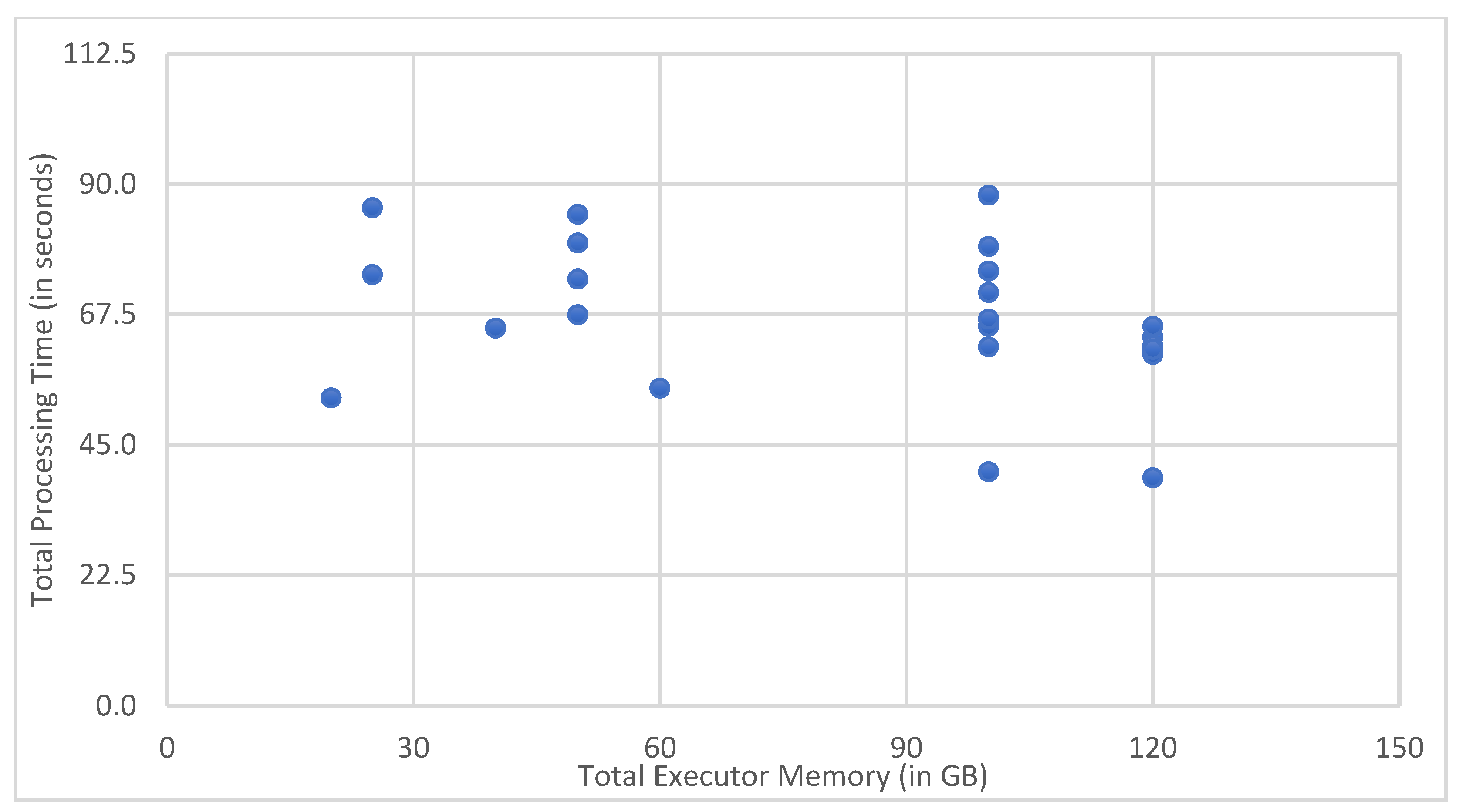
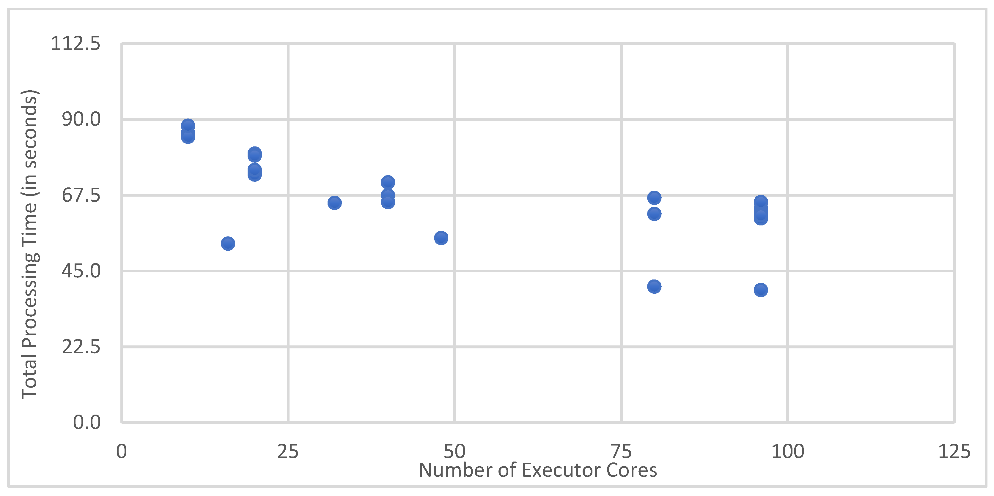
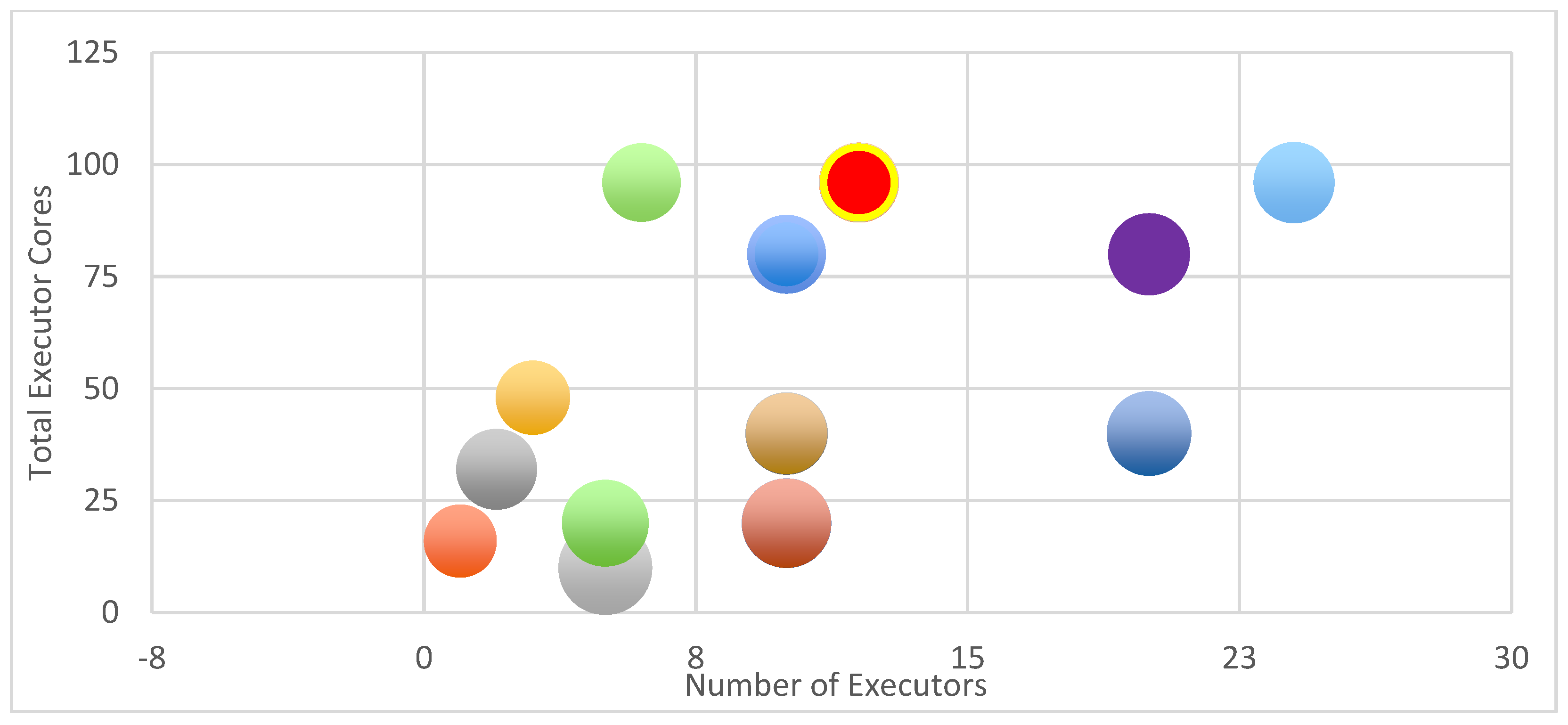
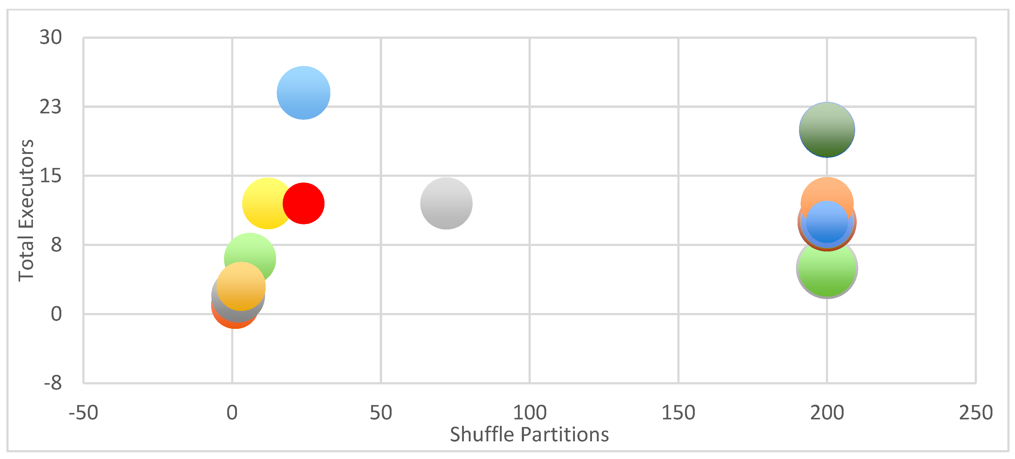
6.1. Determining Spark’s Best Configuration Parameters

To determine Spark’s optimum parameters, using all 18 attributes from the Conn log files of the UWF-ZeekDataFall22 dataset, the DT classifier was used with the following Spark configuration parameters: executor count, executor core count, total executor cores, executor memory, and total executor memory.

Executor count defines the number of executors available for each node [23].

Executor core is the computational power of the CPU. This parameter defines the number of cores available for each executor and the number of concurrent tasks that can be run on each executor [23].

Spark’s executor memory is the amount of memory provided for each executor to complete the task. Defining the executor memory will control the executor heap size and reduce the garbage collection delay [23].

Driver core is the main logic that triggers a Spark job. It is responsible for submitting the job and coordinating the execution of Spark application across the cluster nodes. By default, the number of cores available for a driver program is 1. Using the –driver-cores parameter, we can set up the number of Spark driver cores required for the Spark application [23].

Driver memory is the amount of memory allocated to the driver and basically depends on the number of times we retrieve the data and ranges from 2 GB to 4 GB [23].

Shuffle partition configures the number of partitions to be allocated for shuffling the data while performing RDD operations, such as joins and aggregations. This parameter has no effect when the Spark application has only DataFrame operations [23].

Table 10. UWF-ZeekDataFall22: Binning, training, and testing times for various Spark parameters.

Test ID	Executor Count	Executor Core Count	Total Executor Cores	Executor Memory	Total Executor Memory (GB)	Binning Time (s)	Training Time (s)	Testing Time (s)
1	5	2	10	5	25	69.5	16.4	0.091
2	5	2	10	10	50	69.1	15.6	0.088
3	5	2	10	20	100	71.7	16.2	0.107
4	5	4	20	5	25	59.11	15.13	0.151
5	5	4	20	10	50	58.33	15.16	0.113
6	5	4	20	20	100	59.9	14.91	0.126
7	10	2	20	5	50	63.96	15.77	0.109
8	10	2	20	10	100	63.18	15.94	0.105
9	10	4	40	5	50	54.15	13.15	0.121
10	10	4	40	10	100	52.56	12.788	0.125
11	20	2	40	5	100	57.3	13.84	0.134
12	20	4	80	5	100	51.9	14.7	0.123
13	10	8	80	10	100	49.68	12.09	0.129
14	12	8	96	10	120	50.96	12.54	0.122
15	12	8	96	10	120	49.47	12.54	0.144
16	12	8	96	10	120	47.8	12.6	0.15
17	24	4	96	5	120	50.7	14.5	0.134
18	6	16	96	20	120	46.45	14.87	0.133
19	12	8	96	10	120	28.52	7.94	0.083
20	1	16	16	20	20	44.77	18.25	0.131
21	2	16	32	20	40	46.98	16.57	0.172
22	3	16	48	20	60	38.48	16.7	0.134

shows the impact of varying these parameters on the binning time, training time, and testing time (in seconds).

As can be seen from Table 10, Test 19’s Spark parameters performed the best in terms of binning time, training time, and testing time.

Table 11. UWF-ZeekDataFall22: Total time for additional Spark configuration parameters.

Test ID	Executor Count	Cores Per Executor	Memory per Executor	Total Exec. Cores	Total Executor Memory (GB)	Total Time (s)	Shuffle Partitions	Driver Cores	Driver Memory (GB)
1	5	2	5	10	25	85.93	200	2	10
2	5	2	10	10	50	84.8	200	2	10
3	5	2	20	10	100	88.09	200	2	10
4	5	4	5	20	25	74.41	200	2	10
5	5	4	10	20	50	73.61	200	2	10
6	5	4	20	20	100	74.98	200	2	10
7	10	2	5	20	50	79.84	200	2	10
8	10	2	10	20	100	79.24	200	2	10
9	10	4	5	40	50	67.43	200	2	10
10	10	4	10	40	100	65.44	200	2	10
11	20	2	5	40	100	71.29	200	2	10
12	20	4	5	80	100	66.7	200	2	10
13	10	8	10	80	100	61.91	200	2	10
14	12	8	10	96	120	63.62	200	2	10
15	12	8	10	96	120	62.16	72	2	10
16	12	8	10	96	120	60.6	12	2	10
17	24	4	5	96	120	65.47	24	2	10
18	6	16	20	96	120	61.46	6	2	10
19	12	8	10	96	120	39.33	24	2	10
20	1	16	20	16	20	53.1	1	2	10
21	2	16	20	32	40	65.17	2	2	10
22	3	16	20	48	60	54.79	3	2	10
23	10	8	10	80	100	40.37	200	2	10

shows the effect of varying the driver cores, driver memory, and shuffle partitions on the total time taken by the decision tree classifier. The total time is the sum of binning, training, and testing time. Here, too, Test 19 performed the best.

Figure 2 and Figure 3 show the effects of total executor memory (in GBs) and total number of executor cores on the total processing time (in seconds), respectively. According to Figure 2, there does not appear to be a strong correlation between total executor memory and total processing time. In most runs, increasing the executor memory from 20 to 120 did not reduce the processing time significantly. However, as per Figure 3, the total processing time decreased when the total number of executor cores increased from 10 to 96. The total number of executor cores can be obtained by multiplying the total number of executors with the number of cores per executor.

Figure 4 shows how the total number of executor cores and the number of executors affect the processing time. The size of a bubble indicates the processing time; the smaller the bubble size, the shorter the total processing time. As the total number of executor cores is increased, the bubbles become smaller. The grey bubbles, for example, are large and closer to the x-axis when the number of executor cores is low, indicating higher processing times. The processing time was the shortest for the red bubble, which contained 96 total executor cores and 12 executors.

According to Figure 5, the processing time increases as the shuffle partitions increase. This could be due to the overhead associated with distributing and collecting data over a network. From Figure 4, it can be seen that the processing time was lowest for the red bubble, with 24 shuffle partitions and 12 executors. Hence, Test 18’s Spark configuration parameters from Table 1 were used for testing the classifiers, since this allows for the use of fewer partitions.

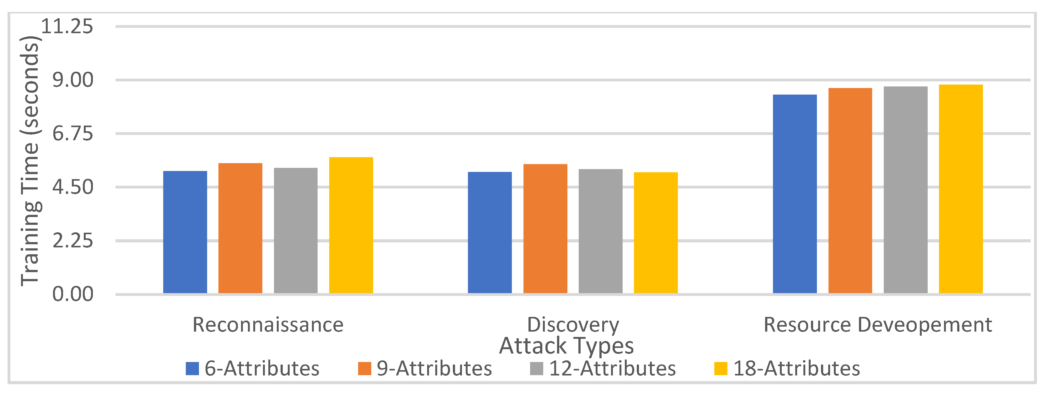
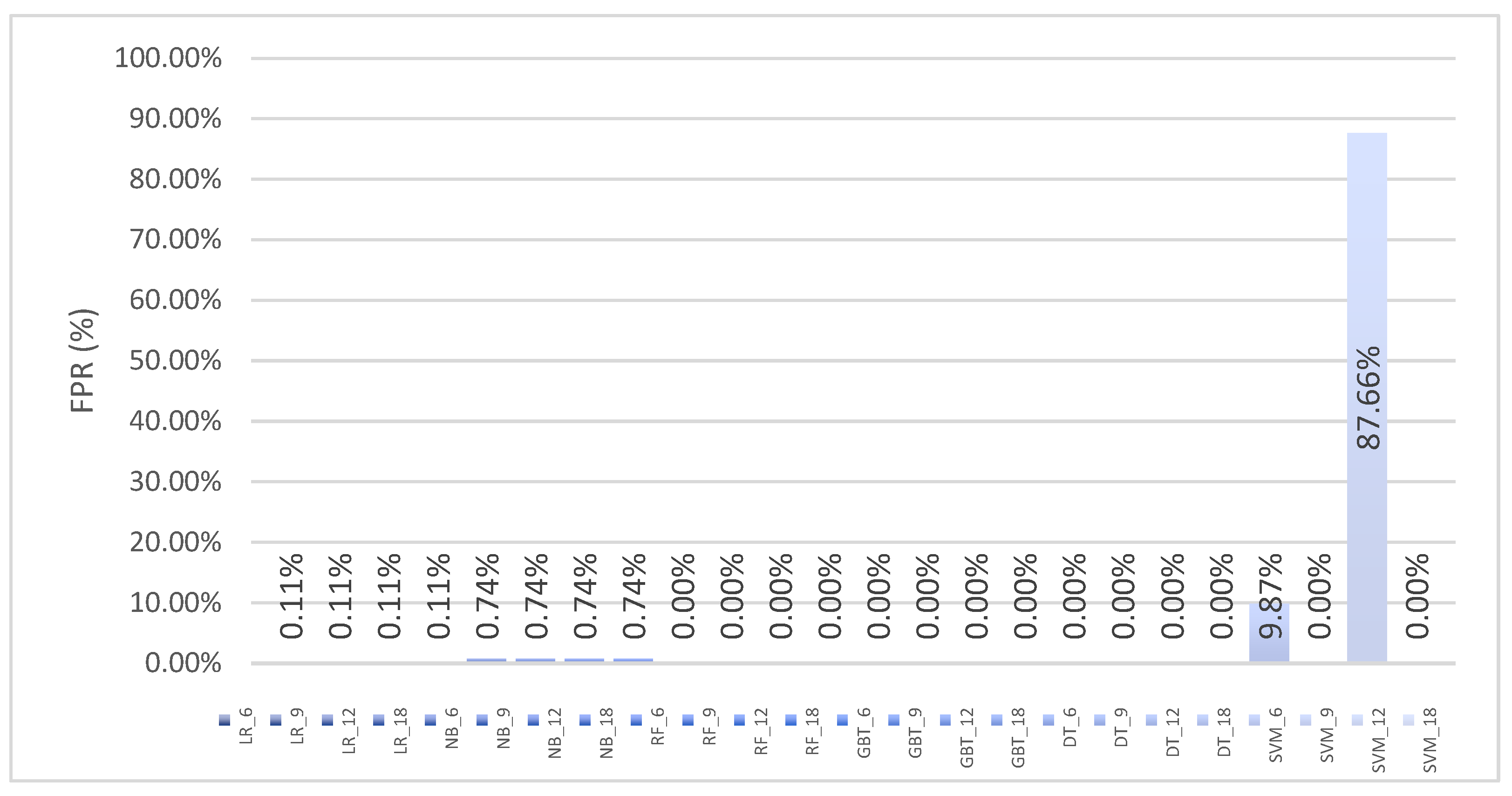
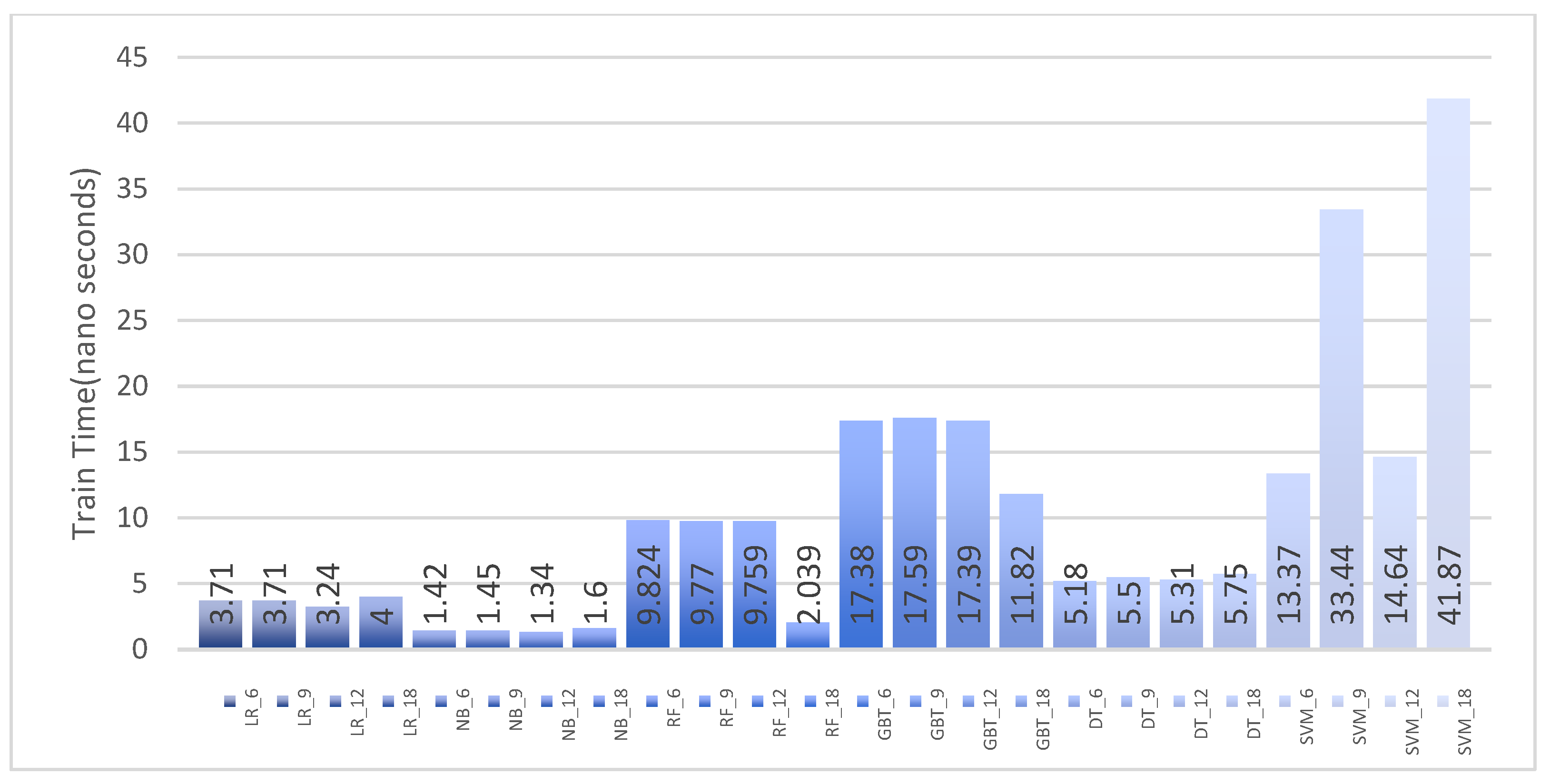
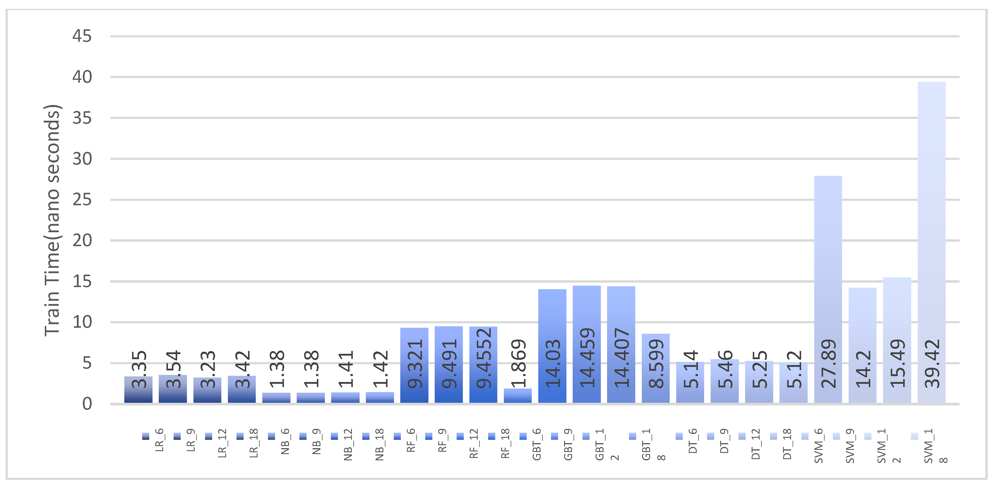
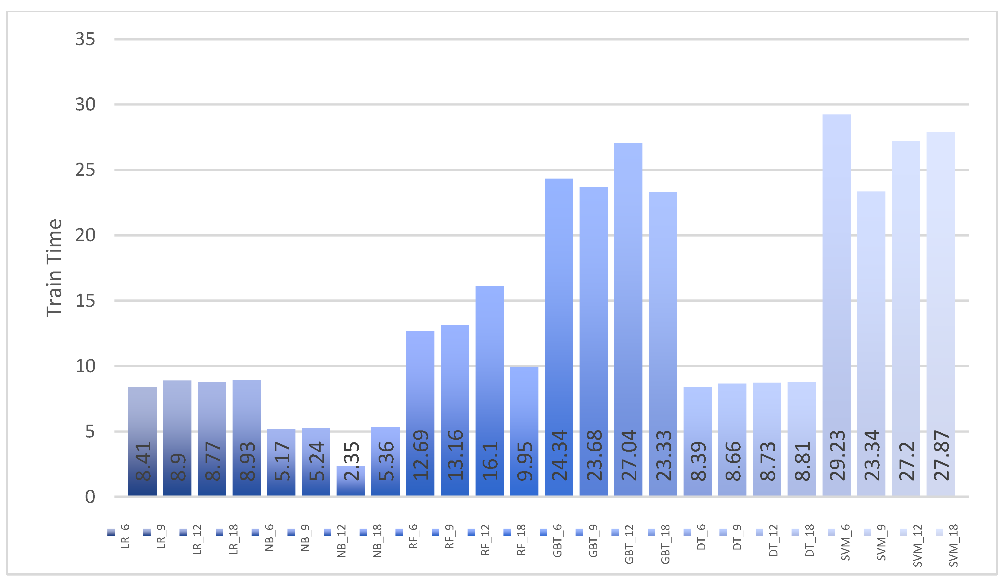
6.2. Analyzing Training Time

The DT classifier was run for 6, 9, 12, and 18 attributes, and the training times were recorded as shown in Figure 6. The six attribute runs were run using the top six attributes from the respective information gain tables, where nine attributes would be the top nine attributes from the respective information gain tables, and so on. There was no significant difference between the number of attributes used with respect to the training time. The training time for resource development was high because of the larger number of records (82,543). The training times for reconnaissance and discovery, however, were low, since there were fewer records.

6.3. Performance of the Machine Learning Classifiers Using UWF-ZeekDataFall22

Six different machine learning classifiers, decision tree, random forest, naïve Bayes, logistic regression, support vector machines, and gradient-boosting trees, were used for classifying the data. Testing was performed on two datasets, UWF-ZeekDataFall22 and UWF-ZeekData22, both available in [12]. The results of the binary classification are presented in

Table 12. UWF-ZeekDataFall22: Binary classification results for the reconnaissance tactic.

ML Algo	# of Attrs.	Accuracy (%)	Precision (%)	Recall (%)	F-Measure (%)	FPR (%)	Training Time (s)	Testing Time(s)
LR	6	99.89	99.74	99.91	99.82	0.11	3.71	0.1
LR	9	99.89	99.74	99.91	99.82	0.11	3.71	0.1
LR	12	99.89	99.74	99.91	99.82	0.11	3.24	0.055
LR	18	99.77	99.73	99.47	99.60	0.11	4	0.098
NB	6	99.33	96.93	99.65	98.27	0.74	1.42	0.044
NB	9	99.33	96.93	99.65	98.27	0.74	1.45	0.09
NB	12	99.33	96.93	99.65	98.27	0.74	1.34	0.086
NB	18	99.33	96.93	99.65	98.27	0.74	1.6	0.089
RF	6	100.00	100.00	100.00	100.00	0.00	9.824	0.103
RF	9	100.00	100.00	100.00	100.00	0.00	9.77	0.087
RF	12	100.00	100.00	100.00	100.00	0.00	9.759	0.099
RF	18	100.00	100.00	100.00	100.00	0.00	2.039	0.08651
GBT	6	100.00	100.00	100.00	100.00	0.00	17.38	0.1101
GBT	9	100.00	100.00	100.00	100.00	0.00	17.59	0.113
GBT	12	100.00	100.00	100.00	100.00	0.00	17.39	0.108
GBT	18	100.00	100.00	100.00	100.00	0.00	11.82	0.112
DT	6	100.00	100.00	100.00	100.00	0.00	5.18	0.13
DT	9	100.00	100.00	100.00	100.00	0.00	5.5	0.09
DT	12	100.00	100.00	100.00	100.00	0.00	5.31	0.14
DT	18	100.00	100.00	100.00	100.00	0.00	5.75	0.14
SVM	6	72.96	82.98	34.96	49.20	9.87	13.37	0.059
SVM	9	80.88	0.00	0.00	0.00	0.00	33.44	0.059
SVM	12	9.97	0.00	0.00	0.00	87.66	14.64	0.069
SVM	18	99.99	100.00	99.91	99.95	0.00	41.87	0.111

,

Table 13. UWF-ZeekDataFall22: Binary classification results for the discovery tactic.

ML Algo.	# of Attrs.	Accuracy (%)	Precision (%)	Recall (%)	F-Measure (%)	FPR (%)	Training Time (s)	Testing Time (s)
LR	6	99.90	99.64	100.00	99.82	0.14	3.35	0.093
LR	9	99.90	99.64	100.00	99.82	0.14	3.54	0.092
LR	12	99.90	99.64	100.00	99.82	0.14	3.23	0.048
LR	18	99.90	99.64	100.00	99.82	0.14	3.42	0.093
NB	6	99.66	96	100.00	99.12	0.41	1.38	0.061
NB	9	99.66	98.26	100.00	99.12	0.41	1.38	0.089
NB	12	98.90	94.99	100.00	97.42	1.24	1.41	0.093
NB	18	98.99	94.96	100.00	97.42	1.24	1.42	0.0875
RF	6	99.90	99.80	100.00	99.90	0.31	9.321	0.099
RF	9	99.90	99.80	100.00	99.90	0.31	9.491	0.1
RF	12	99.90	99.80	100.00	99.90	0.31	9.4552	0.102
RF	18	99.90	99.80	100.00	99.90	0.31	1.869	0.0985
GBT	6	100.00	100.00	100.00	100.00	0.00	14.03	0.1066
GBT	9	100.00	100.00	100.00	100.00	0.00	14.459	0.1016
GBT	12	100.00	100.00	100.00	100.00	0.00	14.407	0.103
GBT	18	100.00	100.00	100.00	100.00	0.00	8.599	0.107
DT	6	100.00	100.00	100.00	100.00	0.00	5.14	0.12
DT	9	100.00	100.00	100.00	100.00	0.00	5.46	0.13
DT	12	100.00	100.00	100.00	100.00	0.00	5.25	0.09
DT	18	100.00	100.00	100.00	100.00	0.00	5.12	0.07
SVM	6	90.87	67.54	100.00	80.62	11.00	27.89	0.06
SVM	9	96.64	99.15	83.03	90.38	0.16	14.2	0.06
SVM	12	82.09	100.00	5.65	10.70	0.00	15.49	0.067
SVM	18	100.00	100.00	100.00	100.00	0.00	39.42	0.08

and

Table 14. UWF-ZeekDataFall22: Binary classification results for the resource development tactic.

ML Algo.	# of Attrs.	Accuracy (%)	Precision (%)	Recall (%)	F-Measure (%)	FPR (%)	Training Time	Testing Time
LR	6	99.87	99.61	99.96	99.78	0.17	8.41	0.118
LR	9	99.87	99.61	99.96	99.78	0.17	8.9	0.118
LR	12	99.87	99.61	99.96	99.78	0.17	8.77	0.068
LR	18	99.85	99.61	99.90	99.75	0.17	8.93	0.136
NB	6	99.33	96.78	99.97	98.35	0.83	5.17	0.053
NB	9	99.33	96.78	99.96	98.35	0.83	5.24	0.096
NB	12	99.34	99.91	99.90	99.38	0.80	2.35	0.089
NB	18	98.55	93.36	99.90	96.52	1.78	5.36	0.104
RF	6	99.99	99.99	100.00	99.99	0.00	12.69	0.17
RF	9	99.99	99.99	100.00	99.99	0.00	13.16	0.12
RF	12	99.99	99.99	100.00	99.99	0.00	16.1	0.0921
RF	18	99.99	99.99	100.00	99.99	0.00	9.95	0.108
GBT	6	100.00	100.00	100.00	100.00	0.00	24.34	0.114
GBT	9	100.00	100.00	100.00	100.00	0.00	23.68	0.113
GBT	12	100.00	100.00	100.00	100.00	0.00	27.04	0.125
GBT	18	100.00	100.00	100.00	100.00	0.00	23.33	0.13
DT	6	100.00	100.00	100.00	100.00	0.00	8.39	0.12
DT	9	100.00	100.00	100.00	100.00	0.00	8.66	0.12
DT	12	100.00	100.00	100.00	100.00	0.00	8.73	0.078
DT	18	100.00	100.00	100.00	100.00	0.00	8.81	0.08
SVM	6	99.87	99.36	99.99	99.68	16.00	29.23	0.06
SVM	9	36.36	3.40	7.00	4.00	54.52	23.34	0.035
SVM	12	36.16	1.70	3.79	2.30	54.78	27.2	0.035
SVM	18	92.12	71.79	99.99	83.57	9.86	27.87	0.034

. The results of the multinomial classification are presented in

Table 15. UWF-ZeekDataFall22: Multinomial classification results.

ML Algo.	No. of Attrs.	Weighted Precision (%)	Weighted Recall (%)	Weighted F-Measure (%)	Weighted Accuracy (%)	FPR (%)	Training Time	Testing Time
LR	6	86.36	92.93	89.52	92.95	92.93	15.8	0.11
LR	9	86.36	92.93	89.52	92.95	92.93	15.95	0.1
LR	12	86.36	92.93	89.52	92.95	92.93	16.3	0.11
LR	18	86.36	92.93	89.52	92.95	92.93	16.55	0.1
NB	6	7.62	0.6235	1.152	8.82	92.18	9.02	0.12
NB	9	7.58	0.622	1.15	8.82	92.18	11.11	0.144
NB	12	7.72	0.672	1.2	9.8	91.1	11.27	0.13
NB	18	7.72	0.672	1.2	9.706	91.1	11.16	0.136
RF	6	99.94	99.97	99.95	99.99	0.0012	35.9	0.099
RF	9	99.94	99.97	99.95	99.99	0.0012	36.6	0.101
RF	12	99.94	99.97	99.95	99.99	0.0012	37	0.1012
RF	18	99.94	99.97	99.95	99.99	0.0012	22.937	0.1
DT	6	99.95	99.97	99.96	99.99	0.0804	13.45	0.104
DT	9	99.95	99.97	99.96	99.99	0.0672	13.91	0.12
DT	12	99.95	99.97	99.96	99.99	0.0737	12.29	0.143
DT	18	99.95	99.97	99.96	99.99	0.0738	13.61	0.128

. The multinomial classification was only performed for the UWF-ZeekDataFall22 dataset.

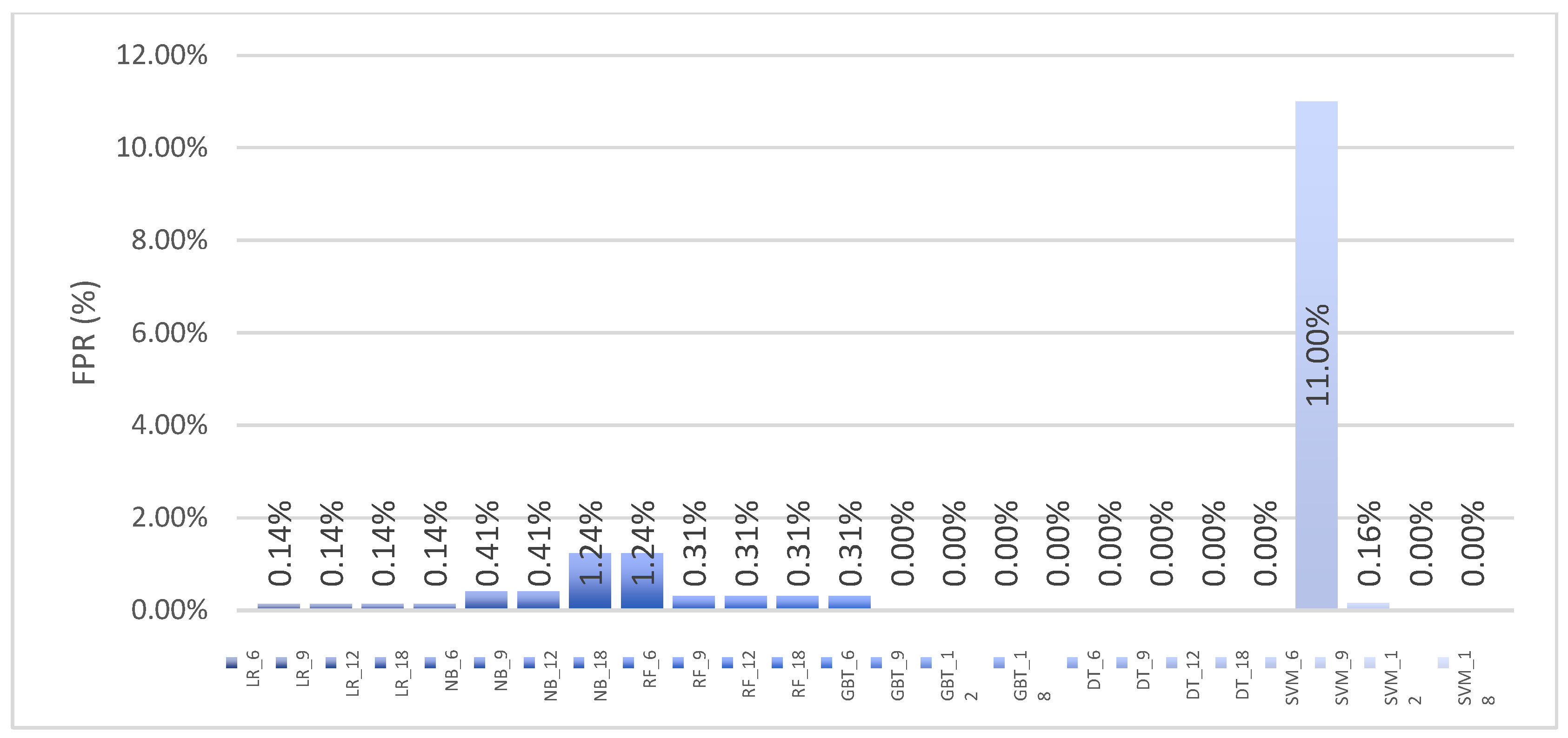
6.3.1. Evaluation Metrics

Classifier performance was measured in terms of accuracy; precision; recall; false positive rate; f-measure; preprocessing time, in terms of binning time; training time; and testing time. Below are some of the commonly used terminologies used in the evaluation metrics:

True Positive (TP): Number of correct positive predictions.

True Negative (TN): Number of correct negative predictions.

False Positive (FP): Number of negative predictions which were incorrectly classified as positive.

False Negative (FN): Number of positive predictions which were incorrectly classified as negative.

Accuracy: Accuracy is the number of correct predictions divided by the total number of predictions:

Accuracy = (TP + TN)/(TP + TN + FP + FN)

(4)

Precision: Precision is the number of correct positive predictions divided by the total number of positive predictions:

Precision = TP/(TP + FP)

(5)

Recall: Recall can be also defined as the true positive rate. It can be calculated as the number of true positives divided by all real positives:

Recall = TP/(TP + FN)

(6)

False Positive Rate (FPR): The FPR is the total number of incorrect positive predictions divided by all real negatives:

FPR = FP/(TN + FP)

(7)

F-Measure: The F-Measure is the harmonic mean of precision and recall:

F-Measure= 2 * (Precision * Recall)/(Precision + Recall)

(8)

Training Time: The time taken by a classifier to train, in seconds.

Testing Time: The time taken by the classifier to perform the predictions, in seconds.

6.3.2. Machine Learning Classifier Results for Binary Classification

Table 12, Table 13 and Table 14 present the binary classification results for all six classifiers using the UWF-ZeekDataFall22 dataset for the reconnaissance, discovery, and resource development tactics, respectively. Binary classification implies using a combination of the respective tactic data with the benign data.

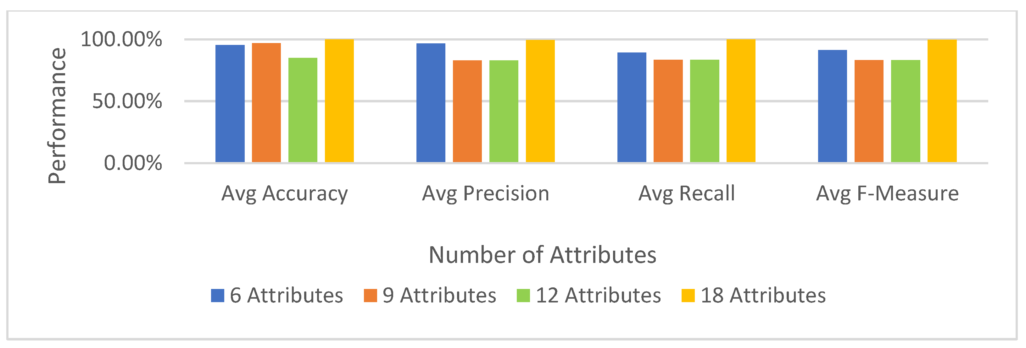
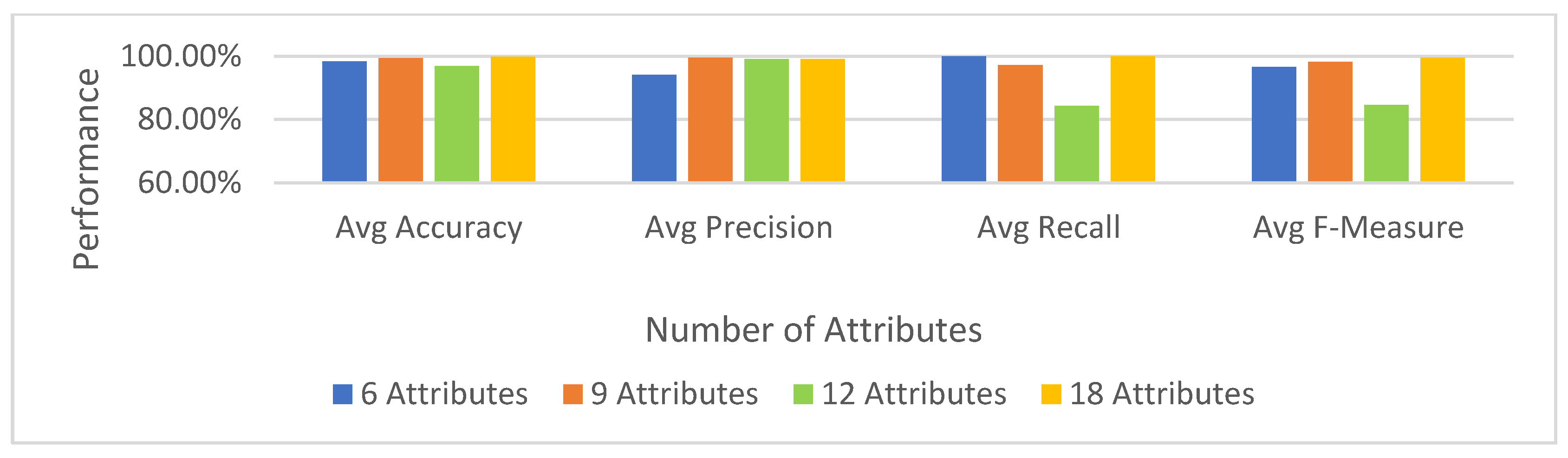
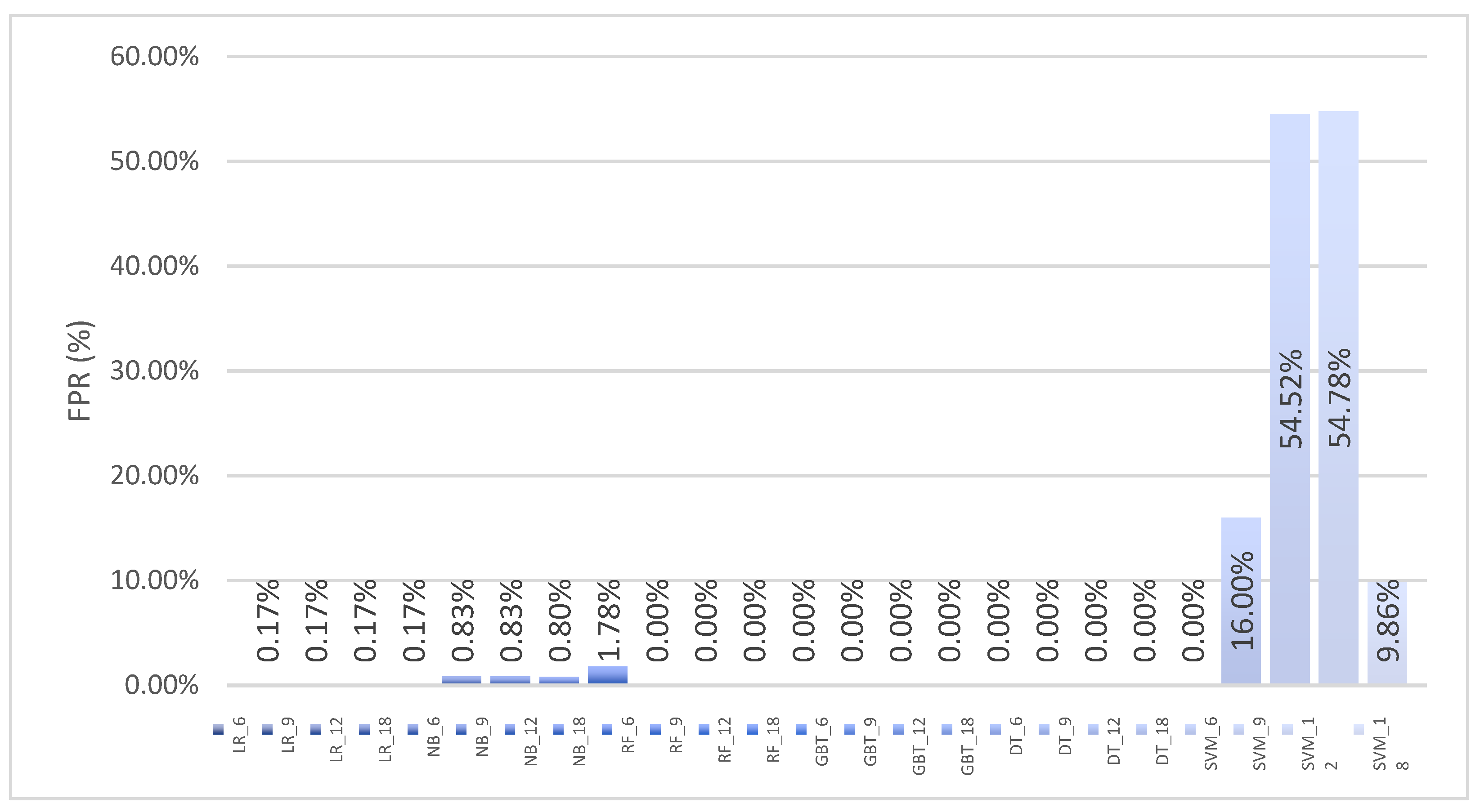
The Reconnaissance Tactic

The results of the binary classification for the reconnaissance tactic using the six different classifiers, LR, NB, RF, GBT, DT, and SVM, are presented in Table 12.

From Table 12, it can be noted that RF, GBT, and DT performed the best, for all combinations of attributes, for accuracy, precision, recall, and the F-measure (all at 100%), although the results of accuracy, precision, and recall were also very close for NB and LR. Except for 18 attributes, SVM did not perform as well, especially for 12 attributes. SVM performed quite poorly in terms of precision, recall, and the F-measure too.

The false positive rates were also relatively high for SVM, especially for 12 attributes, as shown in Figure 7. Again, RF, GBT, and DT have a 0.00% FPR, and LR and NB have a FPR slightly higher than 0.00% (as shown in Table 12 and Figure 7).

In terms of training time, as shown in Figure 8 and Table 12, SVM had a higher overall training time; the second highest was GBT followed by RF and then DT. NB had the lowest training time.

Figure 9 shows the averages for all algorithms by the number of features for the reconnaissance tactic. From Figure 9, the number of features does not seem to have an effect on accuracy, precision, recall, or the F-measure.

The Discovery Tactic

Results of the binary classification for the discovery tactic using the six different classifiers, LR, NB, RF, GBT, DT, and SVM, are presented in Table 13.

From Table 13, it can be noted that GBT and DT performed the best, for all combinations of attributes, for accuracy, precision, recall, and the F-measure, although the results of accuracy, precision, and recall were also very close for RF and LR followed by NB. SVM performed somewhat randomly. SVM performed almost as well for 18 attributes, moderately well for nine attributes, and the worst for 12 attributes.

In terms of recall, all algorithms performed well for all number of attributes except for SVM. In fact, SVM with 12 attributes performed very poorly.

In terms of FPRs, GBT and DT had a rate of 0.00% for all attribute combinations, as shown in Figure 10 as well as in Table 13. Other FPRs were also relatively low except for SVM with six attributes, which had a FPR of 11%.

In terms of training time, SVM had the highest overall training time followed by GBT and then RF, as shown in Figure 11 as well as in Table 13. NB had the lowest training time.

Figure 12 shows the averages for all algorithms according to the number of features for the discovery tactic. From Figure 12, it can be noted that six attributes were relatively low in terms of average precision, and 12 and 18 attributes were relatively low in terms of average recall and the F-measure, respectively.

The Resource Development Tactic

The results of the binary classification for the resource development tactic using the six different classifiers, LR, NB, RF, GBT, DT, and SVM, are presented in Table 14.

Both GBT and DT had 100% accuracy, precision, and recall when tested with the UWF-ZeekDataFall22 dataset using the resource development tactic. In terms of accuracy, the results of the LR, NB, and RF were closely behind GBT and DT, but SVM with nine and 12 attributes performed very poorly compared to the rest. The same pattern can be seen for recall, and the FPRs are shown in Figure 13.

In terms of training time, as can be seen in Figure 14, SVM followed, by GBT, showed the poorest level of performance. Here, NB had the overall lowest training time.

Figure 15 shows the average accuracy, precision, recall, and F-measure of all the algorithms with 6, 9, 12, and 18 attributes. It appears that the averages were relatively higher for six attributes, and the other attributes performed almost the same.

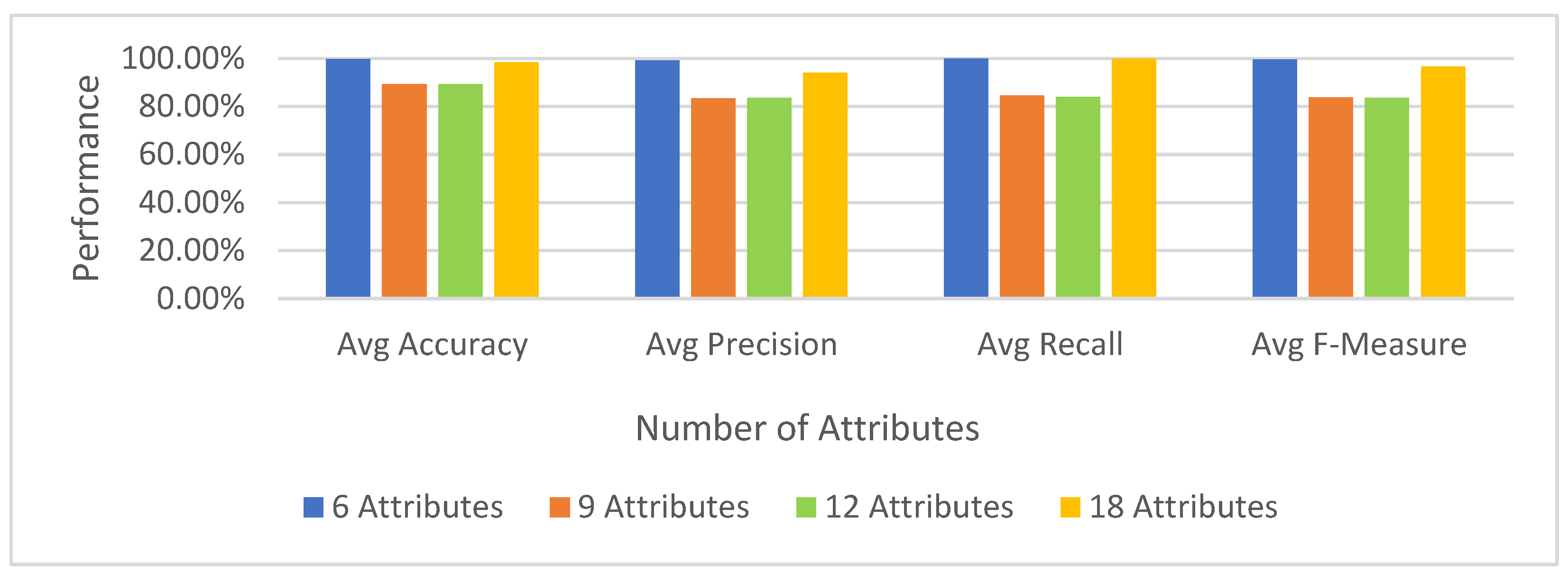
6.3.3. Machine Learning Classifier Results for Multinomial Classification Using the UWF-ZeekDataFall22 Dataset

For multi-classification, the data from the three tactics—reconnaissance, discovery, and resource development—and benign data were used. For multi-classification, weighted accuracy, precision, recall, and the F-measure were used due to the imbalanced nature of the data.

Table 15 presents the multi-classification results for the four classifiers, LR, NB, RF, and DT, using the UWF-ZeekDataFall22 dataset with the four different attribute combinations. Currently, the pyspark MLIb does not support multi-class classification for SVM and GBT and, therefore, these algorithms were not included in the testing.

DT and RF had the highest performance in terms of the weighted precision, weighted recall, weighted F-measure, and weighted accuracy as well as FPR. However, the training time was the highest for the RF classifier. NB had the poorest performance in terms of weighted precision, weighted recall, weighted F-measure, and weighted accuracy.

Binary classification outperformed the multi-classification for all classifiers. Naïve Bayes exhibited very poor performance in the multi-class scenario but achieved an average accuracy of 99.3% with binary classification. The RF and DT classifiers demonstrated good performance in both binary and multi-class classification, making them suitable for both types of classification.

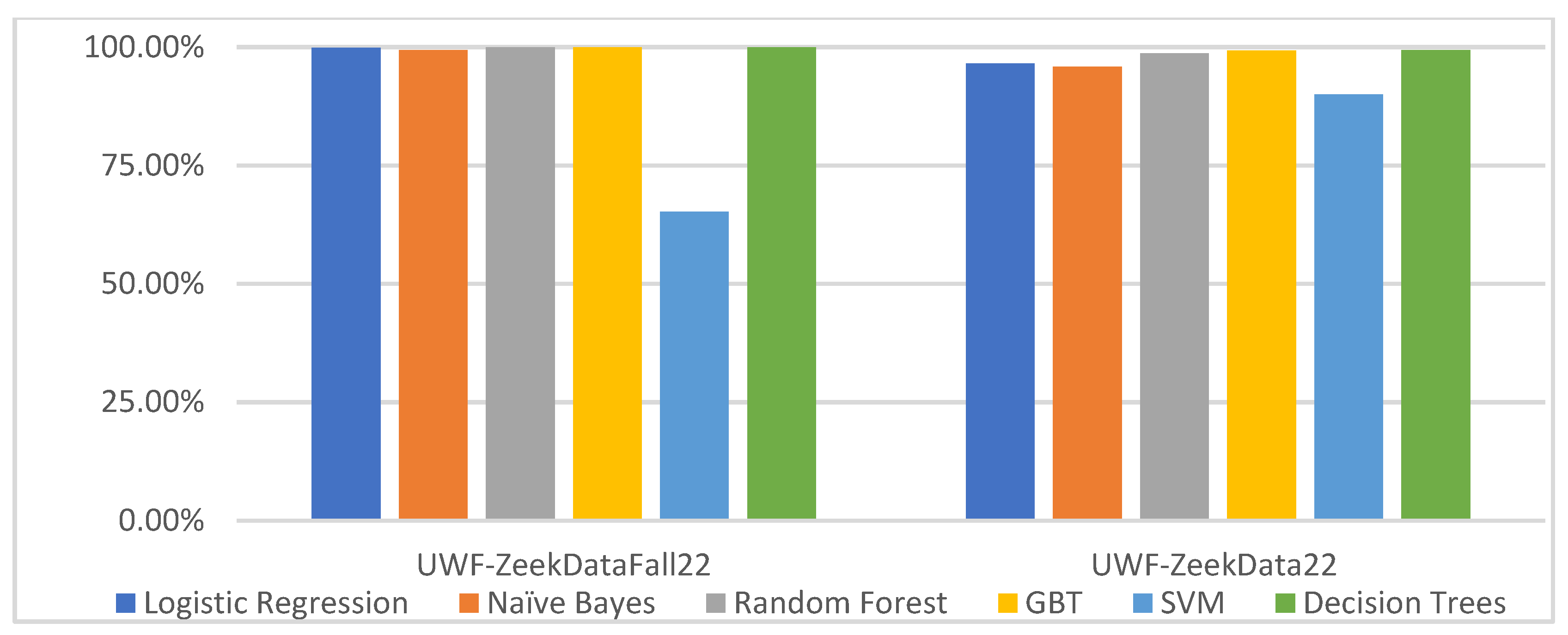
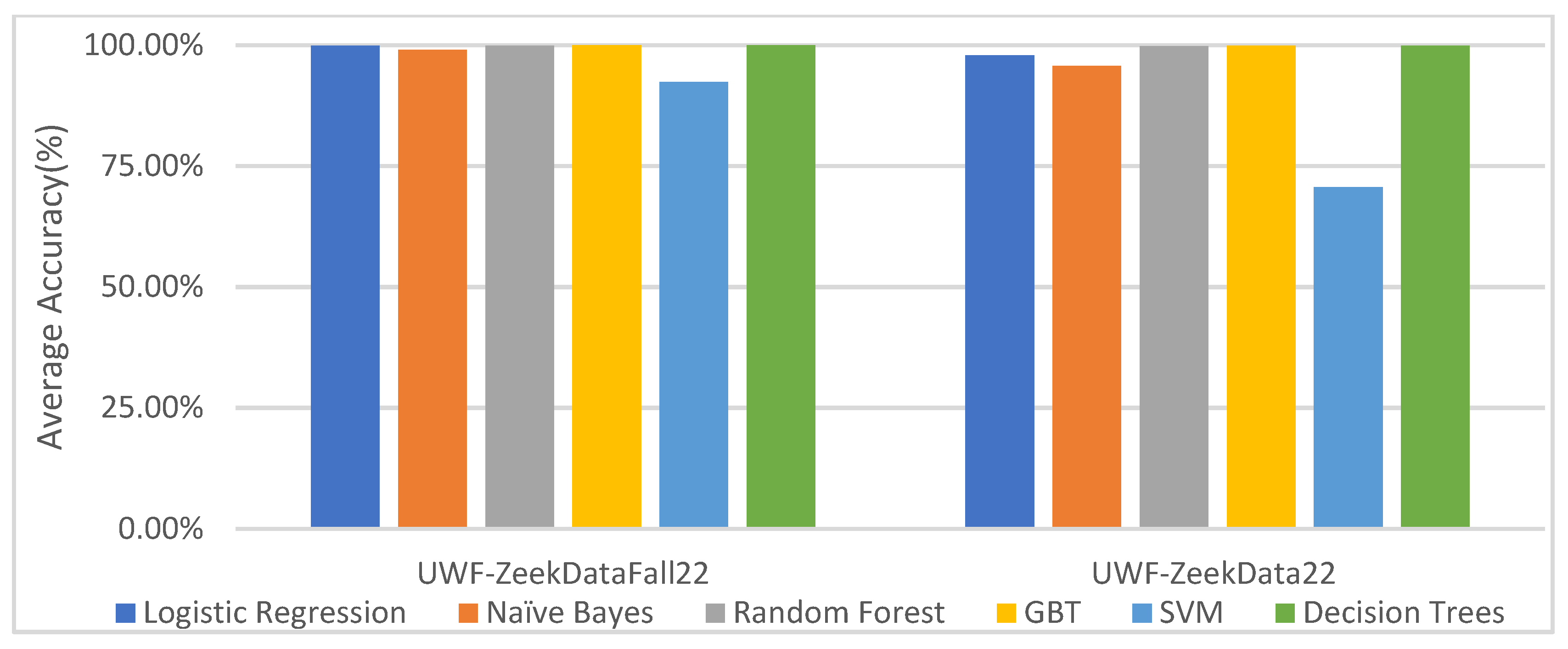
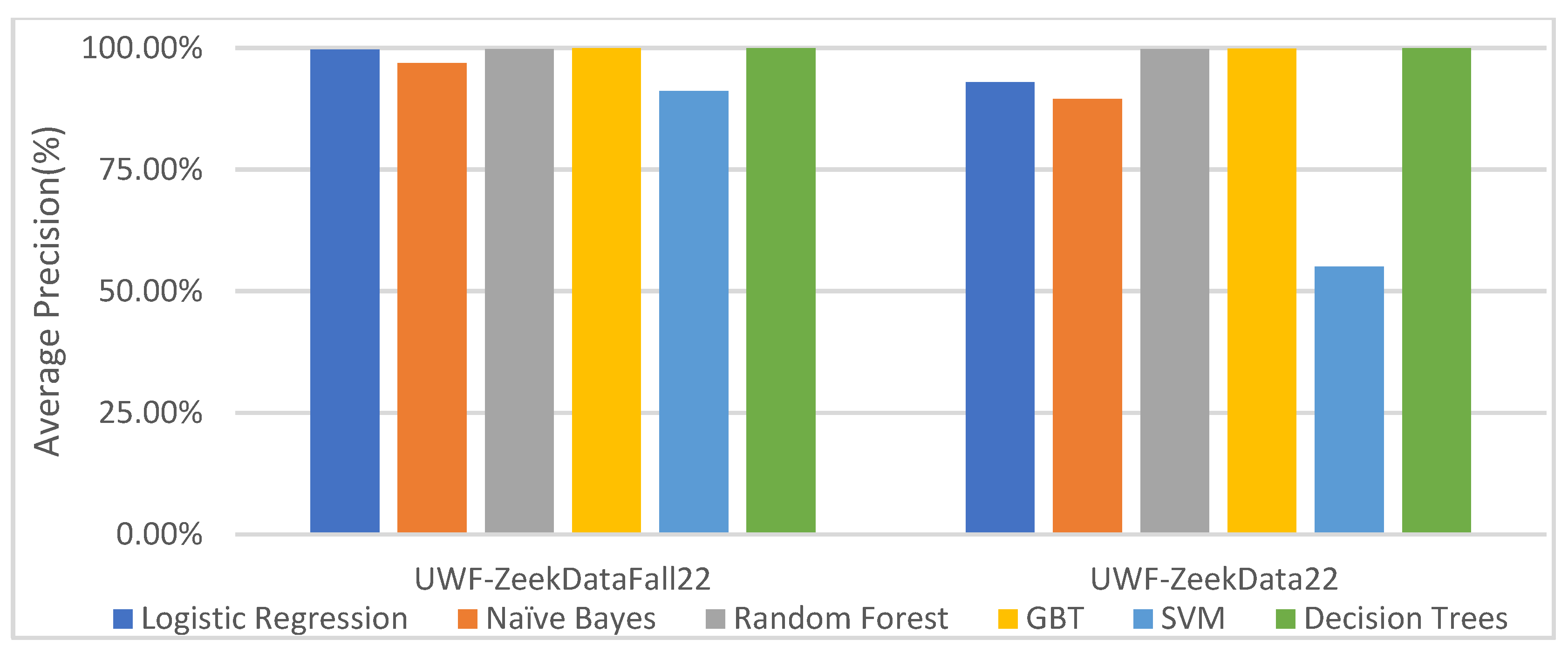
6.3.4. Comparing the UWF-ZeekDataFall22 and UWF-ZeekData22 Datasets

This section compares the results of two datasets, UWF-ZeekDataFall22 and UWF-ZeekData22. The results of the UWF-ZeekData22 dataset can be found in a previously published study [19]. Figure 16 and Figure 17 compare the average binary classification accuracy and precision, respectively, for the reconnaissance tactic using the two different datasets. Figure 18 and Figure 19 compare the average binary classification accuracy and precision, respectively, for the discovery tactic using the two different datasets. These are the averages for all four attribute combinations (6, 9, 12, and 18) for all the classifiers.

Although the results were very close for both reconnaissance and discovery, the average accuracy and precision of all the classifiers except SVM were slightly better using the new UWF-ZeekDataFall22 dataset. RF and DT performed the best for both datasets.

6.4. Limitations of This Study

One major limitation of this study is that, since other tactic datasets are not available, only two datasets could be compared.

7. Summary of Key Findings

Several conclusions can be drawn from this paper. First, in terms of testing Spark’s configuration parameters, there does not appear to be a strong correlation between total executor memory and total process time. Also, the processing time increases as the shuffle partitions increase. This would be due to the overhead associated with distributing and collecting data over a network. From Figure 4, it can be seen that the processing time was lowest with 24 shuffle partitions and 12 executors.

In terms of classification results, it can be noted that, overall, the binary classifiers performed better than the multinomial classifiers, though DT and RF performed almost equally well in the binary as well as the multi-class classifications. For both reconnaissance and discovery, the average accuracy and precision of all the classifiers except SVM was better with the new UWF-ZeekDataFall22 dataset. On average, the multinomial classifiers took longer than the binary classifiers. Finally, overall, the tree-based classifiers performed best in both the binary as well as the multi-class classifications.

Of the three tree-based classifiers, random forest, decision tree, and gradient-boosting tree, the decision tree had the shortest training time for binary classification as well as for multinomial classification for all tactics, and this was the case for all four combinations of attributes. Hence, taking training time into consideration, decision trees can be considered to be the most efficient classifier using Apache Spark, for the UWF-ZeekDataFall22 dataset, labeled as per the MITRE ATT&CK framework.

Elaborating on the high results obtained by the tree-based classifiers, which were at 100% or close to 100%, these results could also be attributed to the successful preprocessing, which reduced the noise in the data. However, it can be noted that SVM performed randomly compared to the other classifiers. Using the UWF-ZeekDataFall22 dataset, for all tactics, SVM performed almost as well for 18 attributes as the other classifiers, and moderately well for 6 or 9 attributes, but performed very poorly for 12 attributes. This needs to be examined further in a future study.

In terms of the number of attributes that performed the best, the top six attributes (as per the information gain measure) performed the best using the resource development tactic. The results using the discovery tactic were not conclusive since both 9 and 18 attributes seemed to perform equally well, in which case 9 attributes would be selected for classification. For the reconnaissance tactic, 6 as well as 18 attributes seemed to perform almost equally well, in which case 6 attributes would be selected for the classification.

8. Conclusions

Data labeled as per the MITRE ATT&CK framework, specifically reconnaissance, discovery, and resource development, are classifiable from Zeek Conn logs using machine learners, specifically decision tree, random forest, gradient-boosting tree, logistic regression, SVM, and naïve Bayes algorithms, although some classifiers perform better than others. They are classifiable using both binary as well a multi-classification framework. Since we obtained the best results with tree-based classifiers (DT, RF, and GBT), our results are also congruent with previous work using network attack data, which showns that RF [12,17] or DT performed best [9,13]. If we take training time into consideration, decision trees can be considered the most efficient classifier for the UWF-ZeekDataFall22 dataset, labeled using the MITRE ATT&CK framework.

References

1. MITRE ATT&CK|MITRE ATT&CK®. Available online: https://attack.mitre.org/# (accessed on 8 August 2023).
2. MITRE ATT&CK. Reconnaissance, Tactic TA0043—Enterprise|MITRE ATT&CK®. 2022. Available online: https://attack.mitre.org/tactics/TA0043/ (accessed on 5 September 2023).
3. MITRE ATT&CK. Discovery, Tactic TA0007—Enterprise|MITRE ATT&CK®. 2022. Available online: https://attack.mitre.org/tactics/TA0007/ (accessed on 5 September 2023).
4. MITRE ATT&CK. Resource Development, Tactic TA0042—Enterprise|MITRE ATT&CK®. 2022. Available online: https://attack.mitre.org/tactics/TA0042/ (accessed on 8 August 2023).
5. University of West Florida. 2022. Available online: https://datasets.uwf.edu/ (accessed on 2 September 2023).
6. Karun, A.K.; Chitharanjan, K. A review on Hadoop—HDFS infrastructure extensions. In Proceedings of the 2013 IEEE Conference on Information and Communication Technologies, Thuckalay, India, 11–12 April 2013. [Google Scholar] [CrossRef]
7. Guller, M. Big Data Analytics with Spark: A Practitioner’s Guide to Using Spark for Large Scale Data Analysis; Apress: New York, NY, USA, 2015. [Google Scholar]
8. About Zeek. Available online: https://docs.zeek.org/en/master/about.html (accessed on 2 August 2023).
9. Mebawondu, O.J.; Popoọla, O.S.; Ayogu, I.I.; Ugwu, C.C.; Adetunmbi, A.O. Network Intrusion Detection Models based on Naives Bayes and C4.5 Algorithms. In Proceedings of the 2022 IEEE Nigeria 4th International Conference on Disruptive Technologies for Sustainable Development (NIGERCON), Lagos, Nigeria, 5–7 April 2022; pp. 1–5. [Google Scholar] [CrossRef]
10. Panda, M.; Patra, M.R. Network Intrusion Detection Using Naïve Bayes. IJCSNS Int. J. Comput. Sci. Netw. Secur. 2007, 7, 258–263. [Google Scholar]
11. Tufail, S.; Batool, S.; Sarwat, A.I. A Comparative Study of Binary Class Logistic Regression and Shallow Neural Network for DDoS Attack Prediction. In Proceedings of the SoutheastCon 2022, Mobile, AL, USA, 26 March–3 April 2022; pp. 310–315. [Google Scholar] [CrossRef]
12. Kejriwal, S.; Patadia, D.; Dagli, S.; Tawde, P. Machine Learning Based Intrusion Detection. In Proceedings of the 2022 IEEE Fourth International Conference on Advances in Electronics, Computers and Communications (ICAECC), Bengaluru, India, 10–11 January 2022; pp. 1–5. [Google Scholar] [CrossRef]
13. Disha, R.A.; Waheed, S. A Comparative study of machine learning models for Network Intrusion Detection System using UNSW-NB 15 dataset. In Proceedings of the 2021 International Conference on Electronics, Communications and Information Technology (ICECIT), Khulna, Bangladesh, 14–16 September 2021; pp. 1–5. [Google Scholar] [CrossRef]
14. Swamy, K.V.R.; Lakshmi, K.V. Network Intrusion Detection Using Improved Decision Tree Algorithm. IJCSIT Int. J. Comput. Sci. Inf. Technol. 2012, 3, 4971–4975. [Google Scholar]
15. Mulay, S.; Devale, P.R.; Garje, G. Intrusion Detection System Using Support Vector Machine and Decision Tree. Int. J. Comput. Appl. 2010, 3, 10–16. [Google Scholar] [CrossRef]
16. Jha, J.; Ragha, L. Intrusion Detection System using Support Vector Machine. In Proceedings of the IJAIS Proceedings on International Conference and Workshop on Advanced Computing (ICWAC), Mumbai, India, 22–23 February 2013; pp. 25–30. [Google Scholar]
17. Belouch, M.; El Hadaj, S.; Idhammad, M. Performance evaluation of intrusion detection based on machine learning using Apache Spark. Procedia Comput. Sci. 2018, 127, 1–6. [Google Scholar] [CrossRef]
18. Bagui, S.S.; Mink, D.; Bagui, S.C.; Ghosh, T.; Plenkers, R.; McElroy, T.; Dulaney, S.; Shabanali, S. Introducing UWF-ZeekData22: A Comprehensive Network Traffic Dataset Based on the MITRE ATT&CK Framework. Data 2023, 8, 18. [Google Scholar] [CrossRef]
19. Bagui, S.S.; Mink, D.; Bagui, S.C.; Ghosh, T.; McElroy, T.; Paredes, E.; Khasnavis, N.; Plenkers, R. Detecting Reconnaissance and Discovery Tactics from the MITRE ATT&CK Framework in Zeek Conn Logs Using Spark’s Machine Learning in the Big Data Framework. Sensors 2022, 22, 7999. [Google Scholar] [CrossRef] [PubMed]
20. Deckert, A.C.; Kummerfeld, E. Investigating the Effect of Binning on Casual Discovery. 2022. Available online: https://arxiv.org/pdf/2202.11789.pdf (accessed on 10 September 2023).
21. Microsoft. TCP/IP Addressing and Subnetting—Windows Client|Microsoft Docs. 2022. Available online: https://docs.microsoft.com/en-us/troubleshoot/windows-client/networking/tcpip-addressing-and-subnetting (accessed on 5 April 2023).
22. IANA. Service Name and Transport Protocol Port Number Registry. 2022. Available online: https://www.iana.org/assignments/service-names-port-numbers/service-names-port-numbers.xhtml (accessed on 5 April 2023).
23. Apache Spark Configuration—Spark 3.3.0 Documentation. 2022. Available online: https://spark.apache.org/docs/latest/configuration.html (accessed on 5 September 2023).
24. Han, J.; Kamber, M.; Pei, J. Data Mining: Concepts and Techniques; Morgan Kaufmann: Burlington, MA, USA, 2022. [Google Scholar]
25. Piryonesi, S.; El-Diraby, T. Data Analytics in Asset Management: Cost-Effective Prediction of the Pavement Condition. J. Infrastruct. Systems. 2020, 26, 04019036. [Google Scholar] [CrossRef]
26. Hastie, T.J.; Tibshirani, R.J.; Friedman, J.H. The Elements of Statistical Learning: Data Mining Inference and Prediction, 2nd ed.; Springer: Berlin/Heidelberg, Germany, 2009; ISBN 978-0-387-84857-0. [Google Scholar]
Figure 1. Overview of the experimentation on the UWF-ZeekDataFall22 dataset.
Electronics 12 05039 g001
Figure 2. UWF-ZeekDataFall22: Total executor memory vs. total processing time.
Electronics 12 05039 g002
Figure 3. UWF-ZeekDataFall22: Total executor cores vs. total processing time.
Electronics 12 05039 g003
Figure 4. UWF-ZeekDataFall22: Processing times varying the numbers of executors and executor cores.
Electronics 12 05039 g004
Figure 5. UWF-ZeekDataFall22: Processing time varying the number of executors and shuffle partitions.
Electronics 12 05039 g005
Figure 6. UWF-ZeekDataFall22: Number of attributes vs. training time.
Electronics 12 05039 g006
Figure 7. UWF-ZeekDataFall22: Reconnaissance: FPR of algorithms according to the number of features used.
Electronics 12 05039 g007
Figure 8. UWF-ZeekDataFall22: Reconnaissance: Training time of algorithms according to the number of features used.
Electronics 12 05039 g008
Figure 9. UWF-ZeekDataFall22: Reconnaissance: Averages for all algorithms according to the number of features.
Electronics 12 05039 g009
Figure 10. UWF-ZeekDataFall22: Discovery: FPR of algorithms according to the number of features used.
Electronics 12 05039 g010
Figure 11. UWF-ZeekDataFall22: Discovery: Training time of algorithms according to the number of features used.
Electronics 12 05039 g011
Figure 12. UWF-ZeekDataFall22: Discovery: Averages for all algorithms according to the number of features.
Electronics 12 05039 g012
Figure 13. UWF-ZeekDataFall22: Resource development: FPRs of algorithms according to the number of features used.
Electronics 12 05039 g013
Figure 14. UWF-ZeekDataFall22: Resource development: Training time of algorithms according to the number of features used.
Electronics 12 05039 g014
Figure 15. UWF-ZeekDataFall22: Resource development: Averages for all algorithms according to the number of features.
Electronics 12 05039 g015
Figure 16. Reconnaissance: Average accuracy of binary classification: UWF-ZeekDataFall22 vs. UWF-ZeekData22.
Electronics 12 05039 g016
Figure 17. Reconnaissance: Average precision of binary classification: UWF-ZeekDataFall22 vs. UWF-ZeekData22.
Electronics 12 05039 g017
Figure 18. Discovery: Average accuracy of binary classification: UWF-ZeekDataFall22 vs. UWF-ZeekData22.
Electronics 12 05039 g018
Figure 19. Discovery: Average precision of binary classification: UWF-ZeekDataFall22 vs. UWF-ZeekData22.
Electronics 12 05039 g019