Communication Time Optimization of Register-Based Data Transfer

Abstract

The data exchange according to communication protocols used in automation is often based on registers (e.g., Modbus). Values of many variables can be sent in a single frame, provided that they are placed in adjacent registers. If the required registers are not adjacent, it may sometimes be advantageous to transmit more registers than required, along with redundant ones, to minimize the number of frames and the total transmission time. The article analyzes the possibilities of improving time parameters and determining the optimal grouping based on the arrangement of registers. Various existing optimization approaches such as mixed integer linear programming, constraint programming, and a tabu search are analyzed, and several new simple deterministic algorithms (greedy or heuristic rule-based) are proposed. The results obtained were confirmed experimentally.

1. Introduction

Communication in distributed automation systems usually uses dedicated industrial networks [1]. These are field networks [2], and, in newer solutions, often industrial Ethernet [3]. In the case of fieldbus networks, the solutions described in the IEC 61158 [4] standard are typically used. There is also a tendency to increasingly use heterogeneous architectures in industrial communication, integrating various types of networks [5], especially in large systems. However, small distributed automation systems are often still based on a serial communication bus (e.g., RS-485) with a protocol such as Profibus or Modbus. In particular, the open Modbus protocol is very popular among manufacturers of small automation devices.

In such types of protocols, the data exchange is usually based on the transfer of registers containing the values of individual variables. The communication protocol typically includes functions to write a single register (e.g., FC6 in Modbus) or multiple registers (e.g., FC16 in Modbus), as well as read several registers (FC3, FC4 in Modbus). The transmission of multiple registers with a single message is usually much faster than the transmission of such registers individually, due to additional time overheads introduced by header fields of the frames. An important limitation during the multiple registers’ transmission is the fact that only a group of adjacent registers may be transmitted together. For this reason, it is sometimes beneficial to send multiple registers in one message, along with some unused registers. The time overhead for the transmission of these redundant registers may be less than the total transmission time of only the necessary registers by separate commands.

The appropriate design of the data exchange scheme can lead to better performance. The idea of grouping registers has been previously described in several articles, briefly presented in Section 2. However, the mentioned articles treat the problem selectively; they usually focus on one protocol, e.g., Modbus, and a specific application, e.g., communication between a PLC and an HMI panel. There is no general approach that is independent of specific protocol and applications. Such a research challenge requires the development of a formal, theoretical definition of the problem, which is achieved in this paper.

It should also be noted that the selection of an optimal grouping is a computationally complex issue. Theoretical considerations require subsequent experimental verification. It is necessary to check the time required for an optimization algorithm to find a solution before it can be applied in practice. The main motivation of this paper is to compare possible optimization techniques in terms of their efficiency, results, and practical applicability. Such an approach was also missing in previous articles. It is worth emphasizing that some of the optimization algorithms, which do not require significant computational power, can be used directly on the PLC, while others are suitable only for offline advance planning on a PC. Our goal was to determine the theoretical and practical usefulness of various optimization approaches, as well as their limits.

The contributions of this paper include the following:

• Formal definition of the problem;
• Development of a fast exact algorithm that can be applied to specific instances of the problem, along with a formal proof of its correctness;
• Development of optimization models based on mathematical programming, namely constraint programming (CP) and mixed-integer linear programming (MILP);
• Dedicated implementation of tabu search (TS) metaheuristic,
• Proposal of three new simple deterministic algorithms, namely the greedy (GR1, GR2) and heuristic rule-based (HR);
• Experimental verification and comparison of the proposed approaches;
• Conclusions on the practical applicability of the analyzed optimization techniques.

The major novelty of this work is the generalized study of the register-based data transfer as an optimization problem. The proposed approach does not restrict the consideration to specific register arrangements, protocols, and  applications. We introduced an original comprehensive formal analysis of the problem along with a theoretical proof (Section 3), and we provided optimization models, as well as proposed several new dedicated algorithms (Section 4). We created a set of original benchmark instances and performed extensive computational experiments (Section 5). Practical guidelines (Section 6) have been derived from the results.

2. Related Work

Articles related to the topic of this paper include the performance analysis of register-based field communication protocols, in particular Modbus, simulations, theoretical analysis, and attempts to improve timing parameters, especially through register grouping.

2.1. Register Grouping

The concept of improving performance through various ways of grouping registers was mentioned in articles [6,7,8,9,10,11,12]. The contributions of each one are briefly summarized below.

In [6], the improvement of the Modbus TCP data exchange between industrial equipment and the HMI system was discussed. The article proposed a method to reduce the update data time by grouping the required slave memory cells into blocks of an optimal length requested via Modbus. Some experimental results of such an approach were also presented and analyzed.

The analysis of the profitability of register grouping for PLC-HMI transmission in Modbus RTU protocol was also described in [7,8] by one of the co-authors of this article. However, the mentioned analysis was quite simple; only two groups of data registers were considered and were separated by a number of redundant registers. In this paper, we consider a more complex and general case with an arbitrary arrangement of multiple registers.

Găitan and Zagan, in their work [9,10], discussed the performance of Modbus communication in various scenarios. They analyzed the impact of accessing multiple registers with consecutive or separated addresses. The extension for the Modbus protocol was also proposed, which provided a new, optimized message format. This extension was experimentally tested, and the results were shown in [11].

In [12], the comparative advantage algorithm for the Modbus protocol was proposed. The message grouping algorithm is one of the therapeutic methods that can restore the functionality of the communication system in the event of an overload of the communication bus.

2.2. Theoretical Analysis

Another group of related works concerns the theoretical analysis of the Modbus protocol [13,14,15].

The formal specifications of the Modbus protocol (request and response messages) can be found in [13]. The formal model was developed using PVS (a generic theorem prover) and SAL (a toolset for the automatic analysis of state-transition systems). This can be observed as the first step in the development of automated methods for systematic and extensive testing of Modbus devices.

Another article [14] presented a time analysis of data exchange in distributed control systems based on the wireless Ethernet network model and the appropriate Modbus protocol. The control system operated in a real-time system, which was responsible for processing periodic and continuous events. The transaction scenario was shown to have a significant impact on the duration of the network cycle and the system response time.

A detailed analysis of the operation of communication networks in experimental studies requires the appropriate tools. Such a tool for analyzing the response time and scheduling of Modbus communication in RS-485 networks was proposed, e.g., in [15]. The response times of a set of messages were collected by a specialized Modbus device and then sent to software where the analysis was performed. Such an approach might lead to an improved performance in a variety of ways. One of them, presented in the aforementioned article, involved the application of different scheduling algorithms. The article proposed a non-preemptive, blocking-free scheduling for networks that require the periodic transmission of a set of independent, low jitter messages.

2.3. Performance Analysis

The final group of references concerns the performance analysis of industrial communication protocols [16,17,18].

In [16], a performance index was proposed to analyze the impact of data transfers on the reliable operation of acquisition systems. The index evaluates the accuracy of the sampling time, taking into account the effects of outliers, bias, and jitter.

The performance of the Modbus TCP protocol was also analyzed in [17]. The article presented the results of simulation studies. The simulations were performed in the NS-3 Network Simulator tool. The performance evaluation focused on the response time, depending on the number of nodes and topology.

In [18], the performance of the Modbus TCP was compared with other industrial Ethernet protocols. Analytic models of EtherCAT, Profinet IRT, Modbus TCP, and Ethernet/IP were proposed to determine the minimum cycle time for each protocol, according to the transmission delay, the network device latency, the propagation delay, the link capacity, the payload, and the number of slaves.

3. Basics of Register-Based Data Transfer

3.1. Problem Statement

In this work, we consider the register-based data transfer problem, specified as follows:

• There is a set of registers to be transferred, each is characterized by its address $r\in \mathbb{N}$, and these addresses are collected in the set R.
• Each register can be either transferred separately or grouped with preceding and/or following registers into a frame for the block transfer.
• The transfer of a single register takes time $\mu$.
• The block transfer time depends on the span of the block, i.e., the transfer time of a block $F\subseteq R$ amounts to $\alpha (\max \left(F\right)-\min \left(F\right)+1)+\beta$.
• These are the following constraints on a problem–solution:

  (a)

  Each register has to be transferred exactly once (separately or in a block);

  (b)

  A block size cannot exceed a predefined upper limit s; if $s=\infty$, then the constraint is omitted and a block can have any size;

• The objective is to find a partition of the register set into separate and block transfers that minimizes the total communication time.

According to the specification, any instance of the problem is characterized by the parameters R, $\mu$, $\alpha$, $\beta$, and s.

Below, we provide concise formal definitions of the problem and its solution, which are a reference for deriving all further optimization models and algorithms.

Definition 1. 

The register-based data transfer problem is defined by a tuple $\mathcal{P}=\left(R,s,\mu ,\alpha ,\beta \right)$, $s\in \mathbb{N}\cup \{\infty \}$, $R\subset \mathbb{N}$, $\mu ,\alpha ,\beta \in \mathbb{R}$, where R contains the addresses of the registers to be transferred, s is the maximum frame size, and μ is the duration of a single register transfer; meanwhile, k-register block transfer time equals $\alpha k+\beta$.

Definition 2. 

Let $\mathcal{P}=\left(R,s,\mu ,\alpha ,\beta \right)$ be a register-based data transfer problem. Its solution is represented by a pair ${\mathcal{S}}_{\mathcal{P}}=\left(A,B\right)$, where

$$A\subseteq R,B=\bigcup _{i=0}^N\left\{[x_i,y_i]\right\},N\in \mathbb{N}\cup \left\{0\right\},x_i,y_i\in R,0<y_i-x_i<s,$$

subject to

$$\left(A\cup \bigcup _{I\in B}I\right)\cap R=R,\bigcup _{I\in B}A\cap I=\varnothing ,\bigcup _{\begin{array}{c}{I}_1,I_2\in B\\ I_1\ne I_2\end{array}}{I}_1\cap I_2=\varnothing .$$

(1)

The set A contains the addresses of the registers to be transferred separately, and the set B contains the ranges of registers for the block transfer.

Note that condition (1) in Definition 2 asserts that each register from R is transferred exactly once. The definition of the set B incorporates the constraint which restricts the span of a block by s.

Given a problem $\mathcal{P}=\left(R,s,\mu ,\alpha ,\beta \right)$ and its solution ${\mathcal{S}}_{\mathcal{P}}=\left(A,B\right)$, a value of the time function $\tau (\mathcal{P},{\mathcal{S}}_{\mathcal{P}})$ representing the total communication time can be calculated

$$\tau (\mathcal{P},{\mathcal{S}}_{\mathcal{P}})=\mu \left|A\right|+\sum _{[x,y]\in B}\left(\alpha (y-x+1)+\beta \right).$$

(2)

The objective of the register-based data transfer problem is to find a solution minimizing the value of the function $\tau (\mathcal{P},{\mathcal{S}}_{\mathcal{P}})$.

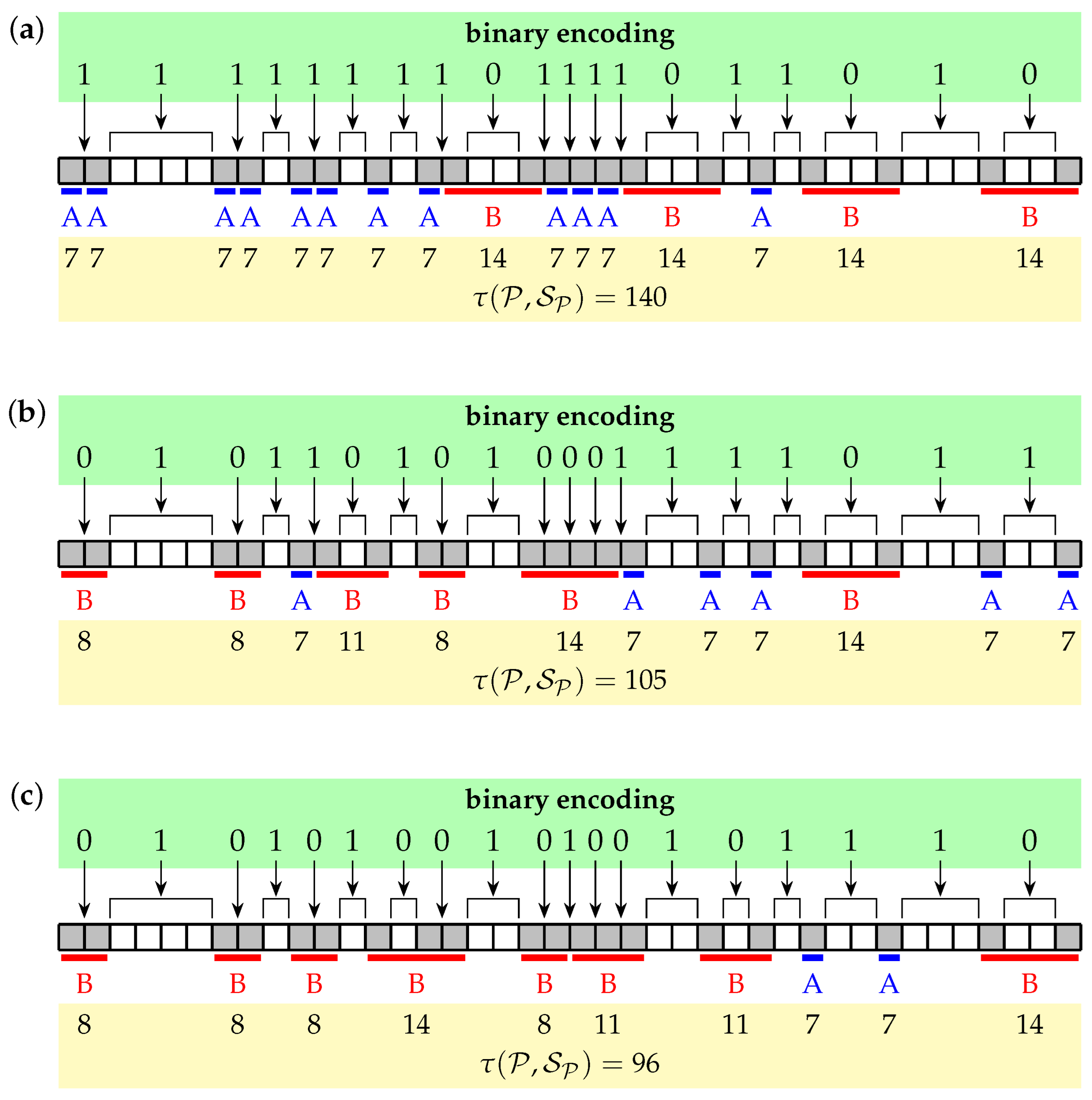
3.2. Binary Solution Encoding

A solution can be equivalently represented by a binary sequence in which, by convention, one represents the separation of consecutive registers, while zeros represent the merging registers into a transfer block.

The notation $\mathfrak{s}\left(X\right)$ will be used for a sequence arranging elements of a set $X\subset \mathbb{N}$ in ascending order, namely $\mathfrak{s}\left(X\right)={\left(x_i\right)}_{i=1}^n$ with $n=\left|X\right|$, such that ${\bigcup }_{i=0}^n\left\{x_i\right\}=X$ and $x_i<x_{i+1}$ for each $i\in \{1,\dots ,n-1\}$.

Definition 3. 

Let ${\mathcal{S}}_{\mathcal{P}}=\left(A,B\right)$ be the solution of a problem $\mathcal{P}=\left(R,s,\mu ,\alpha ,\beta \right)$. Let $n=\left|R\right|$ and ${\left(r_i\right)}_{i=1}^n=\mathfrak{s}\left(R\right)$. The sequence ${\mathcal{B}}_{\mathcal{SP}}={\left(b_i\right)}_{i=1}^{n-1}$, such that

$$b_i=\left\{\begin{array}{cc}0\hfill & \mathit{if}\mathit{there}\mathit{exists}[r_p,r_q]\in B\mathit{such}\mathit{that}p\le i<q,\hfill \\ 1\hfill & \mathit{otherwise},\hfill \end{array}\right.$$

will be referred to as a binary encoding of the solution ${\mathcal{S}}_{\mathcal{P}}$.

The length of the binary encoding for a problem with n registers is equal to $n-1$, so there exists $2^{n-1}$ distinct solutions that have possibly different values of the time function.

3.3. Exemplary Problem Instance

To summarize all the details of the problem specification and solution encoding, we will consider a simple instance of the problem with the parameters: $\mu =7$, $\alpha =3$, $\beta =2$, $s=4$, $R=\{1,2,7,8,10,11,13,15,16,19,20,21,22,23,26,28,30,33,37,40\}$.

Three different solutions to the problem instance are shown in Figure 1, namely the best and the worst one, as well as some intermediate in terms of the value of the objective function $\tau (\mathcal{P},{\mathcal{S}}_{\mathcal{P}})$. The solutions are not unique; there are more groupings with a given maximum (a) or minimum (c) value of the objective function, and only examples of them are presented. The figure shows that the binary encoding determines the points of splitting into frames. As stated in Definition 3, a value of 0 in the encoding means that adjacent registers will be transmitted together; a value of 1 means there is division into separate frames. If a frame consists of one register, it belongs to the set A and is transferred in time $\mu =7$. Otherwise, the frame spans over a block of $k>1$ registers and belongs to the set B; thus, its transfer takes the time $\alpha k+\beta$, i.e., $3k+2$. The sum of transfer times of all frames results in the value of the objective function $\tau (\mathcal{P},{\mathcal{S}}_{\mathcal{P}})$. In this particular example, the frame size limit given by $s=4$ is active in the best solution and prevents merging the registers 19…23 into a single block. It is easy to check that such merging would have improved the result a bit, decreasing the value of $\tau (\mathcal{P},{\mathcal{S}}_{\mathcal{P}})$ from 96 to 93.

The values of parameters of the exemplary problem instance are abstract for legibility. In experiments presented in Section 5, realistic values specific to the Modbus RTU protocol are used.

3.4. Easy Case

If the parameters of the problem meet particular conditions, a special simple solution procedure can be used, as defined by the following theorem.

Theorem 1. 

Let $\mathcal{P}=\left(R,s,\mu ,\alpha ,\beta \right)$ be a problem with $\mu =\alpha +\beta$ and $s=\infty$. Let $n=\left|R\right|$ and ${\left(r_i\right)}_{i=1}^n=\mathfrak{s}\left(R\right)$. Set $\delta =\beta /\alpha +1$. Construct a solution ${\mathcal{S}}_{\mathcal{P}}^{*}$ in which the registers $r_i$, $r_{i+1}$ are transferred in a common frame if $r_{i+1}-r_i<\delta$ and in separate frames if $r_{i+1}-r_i>\delta$ for each $i\in \{1,\dots ,n-1\}$. The ${\mathcal{S}}_{\mathcal{P}}^{*}$ solution is optimal.

Proof. 

Let ${\mathcal{S}}_{\mathcal{P}}$ be an arbitrary solution. Let ${\mathcal{B}}_{\mathcal{SP}}^{*}={\left(b_i^{*}\right)}_{i=1}^{n-1}$ and ${\mathcal{B}}_{\mathcal{SP}}={\left(b_i\right)}_{i=1}^{n-1}$ be the binary encodings of the solutions ${\mathcal{S}}_{\mathcal{P}}^{*}$ and ${\mathcal{S}}_{\mathcal{P}}$, respectively. Set $D=\left\{k\in \mathbb{N}|k<n,b_k\ne b_k^{*}\right\}$.

Fix $i\in D$ and consider the following two as complementary cases.

Case A: $b_i^{*}=0$ and $b_i=1$. In this case, the registers $r_i$ and $r_{i+1}$ are transferred inside a common frame in ${\mathcal{S}}_{\mathcal{P}}^{*}$ and separately in ${\mathcal{S}}_{\mathcal{P}}$. This common frame begins from some register $r_p\le r_i$ and finishes at some register $r_q\ge r_{i+1}$, with the transfer time

$$t_1=\alpha (r_q-r_p+1)+\beta .$$

(3)

In the solution ${\mathcal{S}}_{\mathcal{P}}$, this frame is replaced by two frames, namely from $r_p$ to $r_i$ and from $r_{i+1}$ to $r_q$, hence their net transfer time

$$\begin{array}{cc}\hfill t_2& =\left\{\begin{array}{cc}\mu \hfill & \mathrm{if}{r}_p=r_i\hfill \\ \alpha (r_i-r_p+1)+\beta \hfill & \mathrm{otherwise}\hfill \end{array}\right.\hfill \\ \hfill & +\left\{\begin{array}{cc}\mu \hfill & \mathrm{if}{r}_q=r_{i+i}\hfill \\ \alpha (r_q-r_{i+1}+1)+\beta \hfill & \mathrm{otherwise}\hfill \end{array}\right.\hfill \\ \hfill & \stackrel{\mu =\alpha +\beta }{=}\left(\alpha (r_i-r_p+1)+\beta \right)+\left(\alpha (r_q-r_{i+1}+1)+\beta \right)\hfill \\ \hfill & =\alpha (r_q+r_i-r_p-r_{i+1}+2)+2\beta .\hfill \end{array}$$

(4)

Set ${\Delta }_i^{\mathrm{A}}=t_2-t_1=\alpha (r_i-r_{i+1}+1)+\beta$, and note that $r_{i+1}-r_i\le \delta$, because $r_i$ and $r_{i+1}$ belong to the same frame in ${\mathcal{S}}_{\mathcal{P}}^{*}$; therefore,

$$\begin{array}{cc}\hfill {\Delta }_i^{\mathrm{A}}& =\alpha \left(-(r_{i+1}-r_i)+1\right)+\beta \hfill \\ \hfill & \ge \alpha (-\delta +1)+\beta =\alpha \left(-(\beta /\alpha +1)+1\right)+\beta =0.\hfill \end{array}$$

(5)

Case B: $b_i^{*}=1$ and $b_i=0$. In this case, the registers $r_i$ and $r_{i+1}$ are transferred separately in ${\mathcal{S}}_{\mathcal{P}}^{*}$ and commonly in ${\mathcal{S}}_{\mathcal{P}}$. Hence, there exist registers $r_p\le r_i$ and $r_q\ge r_{i+1}$ such that the frames from $r_p$ to $r_i$ and from $r_{i+1}$ to $r_q$ belong to ${\mathcal{S}}_{\mathcal{P}}^{*}$; their counterpart in ${\mathcal{S}}_{\mathcal{P}}$ is the frame from $r_p$ to $r_q$. As a result, the values $t_1$ and $t_2$ from (3) and (4) swap, leading to ${\Delta }_i^{\mathrm{B}}=t_2-t_1=\alpha (r_{i+1}-r_i-1)-\beta$. The registers $r_i$ and $r_{i+1}$ belong to different frames in ${\mathcal{S}}_{\mathcal{P}}^{*}$; therefore, $r_{i+1}-r_i\ge \delta$ and

$$\begin{array}{cc}\hfill {\Delta }_i^{\mathrm{B}}& =\alpha \left((r_{i+1}-r_i)-1\right)-\beta \hfill \\ \hfill & \ge \alpha (\delta -1)-\beta =\alpha \left((\beta /\alpha +1)-1\right)-\beta =0\hfill \end{array}$$

(6)

Note that ${\Delta }_i^{\mathrm{A}}$ or ${\Delta }_i^{\mathrm{B}}$ specifies the change of time function value when a solution is modified by toggling $b_i^{*}$. Also note that ${\Delta }_i^{\mathrm{A}}$ and ${\Delta }_i^{\mathrm{B}}$ remain valid when recursively merging many such changes for distinct $i\in D$, as the recursion may affect only the values of $r_p$ and $r_q$ that are not present in (5) and (6). In particular, by merging the changes for all $i\in D$, the solution ${\mathcal{S}}_{\mathcal{P}}^{*}$ is transformed into ${\mathcal{S}}_{\mathcal{P}}$, hence

$$\tau (\mathcal{P},{\mathcal{S}}_{\mathcal{P}})=\tau (\mathcal{P},{\mathcal{S}}_{\mathcal{P}}^{*})+\sum _{i\in D}\left\{\begin{array}{cc}{\Delta }_i^{\mathrm{A}}\hfill & \mathrm{if}{b}_i^{*}=0,\hfill \\ {\Delta }_i^{\mathrm{B}}\hfill & \mathrm{if}{b}_i^{*}=1.\hfill \end{array}\right.$$

(7)

Combining (5), (6), and (7), one obtains $\tau (\mathcal{P},{\mathcal{S}}_{\mathcal{P}}^{*})\le \tau (\mathcal{P},{\mathcal{S}}_{\mathcal{P}})$.    □

The solving procedure described in the statement of Theorem 1 is easy to implement but, first of all, it has a low computational complexity. It involves $n-1$ operations on the register pairs $(r_i,r_{i+1})$, and every such operation does not depend on n; thus, the overall time complexity is $O\left(n\right)$. Having ${\mathcal{B}}_{\mathcal{SP}}^{*}$, one needs to calculate $\tau (\mathcal{P},{\mathcal{S}}_{\mathcal{P}}^{*})$, which can be performed using the algorithm from Algorithm 1, which also has the execution time asymptotically proportional to n. Therefore, the overall optimization is relatively fast and has the time complexity $O\left(n\right)$.

Algorithm 1: Calculation of the time function value $\tau (\mathcal{P},{\mathcal{S}}_{\mathcal{P}})$

3.5. General Case

In a general case, if the assumptions from Theorem 1 are not satisfied, the easy and fast solving procedure does not assert an optimal or even feasible solution. One can then perform an exhaustive search of the whole solution space, but such an algorithm has the impractical time complexity $O\left(2^n\right)$. Tests revealed that such a brute force approach is useful for problems with $\left|R\right|$ up to 30…40, depending on CPU performance and optional parallelization of processing. For example, the optimization time as a function of the number of registers shown in Figure 2 has been obtained using Ryzen 9 3900X 12-Core CPU (AMD, Santa Clara, CA, USA) and single thread computation. It grows exponentially from about 3 ms for $\left|R\right|=16$ to about 1 h for $\left|R\right|=36$.

For larger instances, the exhaustive search is useless, and more advanced optimization approaches are required. We have chosen two mathematical programming techniques, namely MILP and constraint programming, which are widely used for hard optimization problems. We have also implemented the tabu search metaheuristic which can often overperform mathematical programming solvers due to use of problem encoding dedicated directly for a specific case [19,20]. Finally, we have developed deterministic algorithms based on greedy or heuristic rules which are guided by locally defined optima rather than the global objective function; hence, they may be less efficient at objective minimization, but competitive in industrial applications due to simple implementation and low computational complexity. All the optimization approaches are described in detail in the next section.

4. Optimization Approaches

4.1. Mixed Integer Linear Programming

The first optimization approach is based on mixed integer linear programming (MILP). It is a well-known approach supported by many software tools.

The MILP model involves the following decision variables

• $f_{i,j}\in \{0,1\}$, $(i,j)\in {\{1,\dots ,n\}}^2$—equals 1 if, and only if, the register $r_i$ is transmitted in the j-th frame;
• $u_i\in \{0,1\}$, $i\in \{1,\dots ,n\}$—equals 1 if and only if the i-th frame is used, i.e., the total number of frames is not less than i;
• $l_i\in \{0,1\}$, $i\in \{1,\dots ,n\}$—equals 1 if, and only if, the i-th frame contains exactly one register;
• ${\underline{r}}_i,{\overline{r}}_i\in \{min\left(R\right),\dots ,max\left(R\right)\}$, $i\in \{1,\dots ,n\}$—the first and the last register, respectively, transmitted inside the i-th frame;
• $w_i\in \{0,\dots ,s\}$, $i\in \{1,\dots ,n\}$—the size of the i-th frame, i.e., the number of registers it includes;
• $t_i\in [0,\mu n]$, $i\in \{1,\dots ,n\}$—the time of transmission of the i-th frame.

The goal is to minimize the objective function ${\sum }_{i=1}^n{t}_i$ subject to

$$\sum _{j=1}^n{f}_{i,j}=1,i\in \{1,\dots ,n\},$$

(8)

$${\underline{r}}_j\le r_i+(1-f_{i,j})M,(i,j)\in {\{1,\dots ,n\}}^2,$$

(9)

$${\overline{r}}_j\ge r_i-(1-f_{i,j})M,(i,j)\in {\{1,\dots ,n\}}^2,$$

(10)

$$w_i\ge {\overline{r}}_i-{\underline{r}}_i+1,i\in \{1,\dots ,n\},$$

(11)

$$w_i\le s-l_i(s-1),i\in \{1,\dots ,n\},$$

(12)

$$t_i\ge (l_i+u_i-1)\mu ,i\in \{1,\dots ,n\},$$

(13)

$$t_i\ge \alpha w_i+\beta -(l_i-u_i+1)\mu n,i\in \{1,\dots ,n\},$$

(14)

$$u_{i+1}\le u_i,i\in \{1,\dots ,n-1\},$$

(15)

$${\underline{r}}_{i+1}\ge {\overline{r}}_i+1,i\in \{1,\dots ,n-1\},$$

(16)

$$f_{i,j}\le u_j,(i,j)\in {\{1,\dots ,n\}}^2,$$

(17)

$$w_i\le u_{i}s,i\in \{1,\dots ,n\}.$$

(18)

The symbol M in (9) and (10) is a large enough constant, and the value $M=max\left(R\right)-min\left(R\right)+1$ is sufficient in practice. If $s=\infty$ in $\mathcal{P}$, one should also use M instead of s in (12) and (18).

Each register is assigned to exactly one frame (8). The lower and upper bounds of the frames, i.e., ${\underline{r}}_i$ and ${\overline{r}}_i$, are constrained by the registers assigned to them in (9) and (10). Frame sizes are bounded from below by the assigned registers (11) and bounded from above by 1 or s, according to the values of $l_i$ (12). If the i-th frame includes one register ($u_i=1$, $l_i=1$), its time $t_i$ is forced to not be less than $\mu$ (13). Otherwise, if the frame includes many registers ($u_i=1$, $l_i=0$), the time value not less than $\alpha w_i+\beta$ is forced (14).

The remaining constraints (15)–(18) are not necessary for model completeness; however, they break the solution space symmetry or advise shortcut relationships between variables. They have been experimentally confirmed to improve the optimization performance.

4.2. Constraint Programming

The constraint programming model uses binary decision variables $b_i\in \{0,1\}$, $i\in \{1,\dots ,n\}$, which are direct elements of the binary solution encoding ${\mathcal{B}}_{\mathcal{SP}}$ from Definition 3. Variables ${\underline{r}}_i$ and ${\overline{r}}_i$ are also used and defined identically to the previous section.

A few auxiliary decision expressions are defined for each $i\in \{1,\dots ,n\}$

$$\begin{array}{cc}\hfill & {\kappa }_i:=1+\sum _{j=1}^{i-1}{b}_j,\hfill \end{array}$$

(19)

$$\begin{array}{cc}\hfill & {\omega }_i:={\overline{r}}_i-{\underline{r}}_i+1,\hfill \end{array}$$

(20)

$${\epsilon }_i:=\left\{\begin{array}{cc}1\hfill & \mathrm{if}{\omega }_i=1,\hfill \\ 0\hfill & \mathrm{otherwise},\hfill \end{array}\right.{\gamma }_i:=\left\{\begin{array}{cc}1\hfill & \mathrm{if}{\omega }_i>1,\hfill \\ 0\hfill & \mathrm{otherwise}.\hfill \end{array}\right.$$

(21)

The goal is to minimize the objective expression

$$f:=\sum _{i=1}^n\left({\epsilon }_i\mu +{\gamma }_i(\alpha w_i+\beta )\right)$$

(22)

subject to

$$\begin{array}{cccc}\hfill & {\underline{r}}_{\left[{\kappa }_i\right]}\le r_i,{\overline{r}}_{\left[{\kappa }_i\right]}\ge r_i,\hfill & \hfill & i\in \{1,\dots ,n\},\hfill \end{array}$$

(23)

$$\begin{array}{cccc}\hfill & {\omega }_i\le s,\hfill & \hfill & i\in \{1,\dots ,n\}.\hfill \end{array}$$

(24)

The notation $x_{\left[y\right]}$ represents the dynamic selection of the y-th element of the sequence x, where both y and the elements of x are decision variables or expressions. Such dynamic indexing is commonly supported by constraint programming solvers, and thid has made it possible to implement the problem in a more concise way compared to the MILP model. According to (19), we have ${\kappa }_i=k$ for $i\in I_k=\{p,\dots ,q\}\subseteq \{1,\dots ,n\}$ such that the registers $\{r_p,\dots ,r_q\}\subseteq R$ are to be transferred in the k-th consecutive frame. As a consequence, the constraints (23) obtain the form ${\underline{r}}_k\le r_i$ and ${\overline{r}}_k\ge r_i$ for $i\in I_k$, which implies that the value $r_q-r_p+1$ will be assigned to ${\omega }_k$, according to (20). There are expressions (20) reserved for the maximum possible number of frames equal to n, but not all of them are needed in a typical solution, and then ${\kappa }_n<n$. In such a case, no constraints are activated for ${\underline{r}}_k$, ${\overline{r}}_k$ with $k>{\kappa }_n$, according to (23). As a result, the solver can freely choose the ${\underline{r}}_k$ and ${\overline{r}}_k$ values giving ${\omega }_k\le 0$ in (20), hence ${\epsilon }_k={\gamma }_k=0$ in (21), and the k-th frame does not contribute to (22). The maximum frame sizes are limited in (24), and these restrictions should be removed if $s=\infty$.

4.3. Tabu Search

The tabu search is a quite popular metaheuristic that extends the basic local search procedure. It has been introduced by Glover [21,22]. The main idea is to forbid visiting solutions that have been checked recently. Such solutions are remembered using attributes stored in the so-called tabu list. This tabu mechanism prevents the search for stacking in a loop trajectory and generally enhances the exploratory ability of the algorithm. The tabu search usually offers a relatively good performance despite a simple implementation. Its advantage is also that the balance between speed and solution quality can be easily adjusted by the design of a neighborhood structure. The tabu search algorithm implemented for the register-based data transfer problem is characterized by the following details:

• A solution is coded by binary encoding (Definition 3).
• The binary encoding words are also used as tabu attributes stored in the tabu list.
• The value of the objective function is calculated using the procedure from Algorithm 1. Solutions with an exceeding frame length are dropped, so that the algorithm visits only the feasible solutions.
• The move, i.e., an elementary modification of a solution in the neighborhood, is defined as toggling one bit of the binary encoding word.
• The neighborhood consists of moves based on every encoding bit. In other words, the solution represented by a binary encoding ${\mathcal{B}}_{\mathcal{SP}}={\left(b_i\right)}_{i=1}^{n-1}$ has $n-1$ neighbor solutions in the set

  $$N\left({\mathcal{B}}_{\mathcal{SP}}\right)=\bigcup _{j=1}^{n-1}\left\{{\left(c_i\right)}_{i=1}^{n-1}|c_i=(1-{\delta }_{i,j})b_i+{\delta }_{i,j}(1-b_i)\right\},$$

  where ${\delta }_{i,j}$ is the Kronecker symbol.
• The algorithm does not necessarily use the full neighborhood $N\left({\mathcal{B}}_{\mathcal{SP}}\right)$, but any of its elements are accepted with the probability $p^{\mathrm{TS}}$ and rejected otherwise. This improves the stochastic nature of the search and supports escaping from loops, if the tabu mechanism is insufficient.
• The standard aspiration criterion is implemented, meaning that a new solution overperforming the current global optimum is always accepted, even if it is forbidden by the tabu list.
• The initial solution is generated randomly.

The tabu search algorithm requires two configuration parameters to be set, which are the probability of acceptance of a move $p^{\mathrm{TS}}$ and the length of the tabu list $l^{\mathrm{TS}}$.

4.4. Deterministic Algorithms

Three deterministic algorithms have also been implemented. They run very fast compared to those previously presented, as their logic is based on simple rules.

The first algorithm Greedy 1 (GR1) merges registers in the largest possible frames. Frames are split only if the maximum frame size is to be exceeded. The pseudocode of the algorithm is given in Algorithm 2. A binary encoding with all merged registers is created first (line 1). Then, consecutive registers are iterated (line 3), and the current frame is closed (line 5) if it cannot be longer (line 4).

Algorithm 2: Pseudocode of algorithm GR1

A quite similar algorithm, Greedy 2 (GR2) from Algorithm 3 was also developed. In this case, however, frames are not split just before the length is exceeded, but the algorithm traces back to the nearest gap between registers that is the largest in the current frame (line 7). The largest gap size is stored in $\gamma$ and its position in $\pi$ (lines 4–5).

Algorithm 3: Pseudocode of algorithm GR2

The algorithm GR1 better minimizes the number of frames, while GR2 may generate more frames, but they are split in better places. It is hard to predict in advance which one will be better for a given problem instance, thus both may be applied and compared.

The algorithms GR1 and GR2 are suitable for the instances where registers are close to each other enough and their merging is profitable. In general, a better strategy may be to split registers if the gaps between them exceed some threshold. This threshold is well defined only for special conditions established in Theorem 1; however, it can be extrapolated heuristically for a general case. It leads to the third Heuristic Rule-based (HR) algorithm. Its pseudocode is presented in Algorithm 4. First, the set $\Gamma$ of all gap values between registers is built (line 1). For each $\gamma \in \Gamma$ (line 3), the algorithm constructs a solution with frames divided between registers that have a gap not less than $\gamma$ (lines 7–8). However, there is no guarantee that these frames do not exceed the length limit. For that reason, each of the frames including more than one register is additionally split (if needed) by the algorithm GR2 (line 9). For each constructed solution, the objective function value is calculated (line 13) using the procedure from Algorithm 1. A solution minimizing the objective is returned as the algorithm result (lines 14, 16).

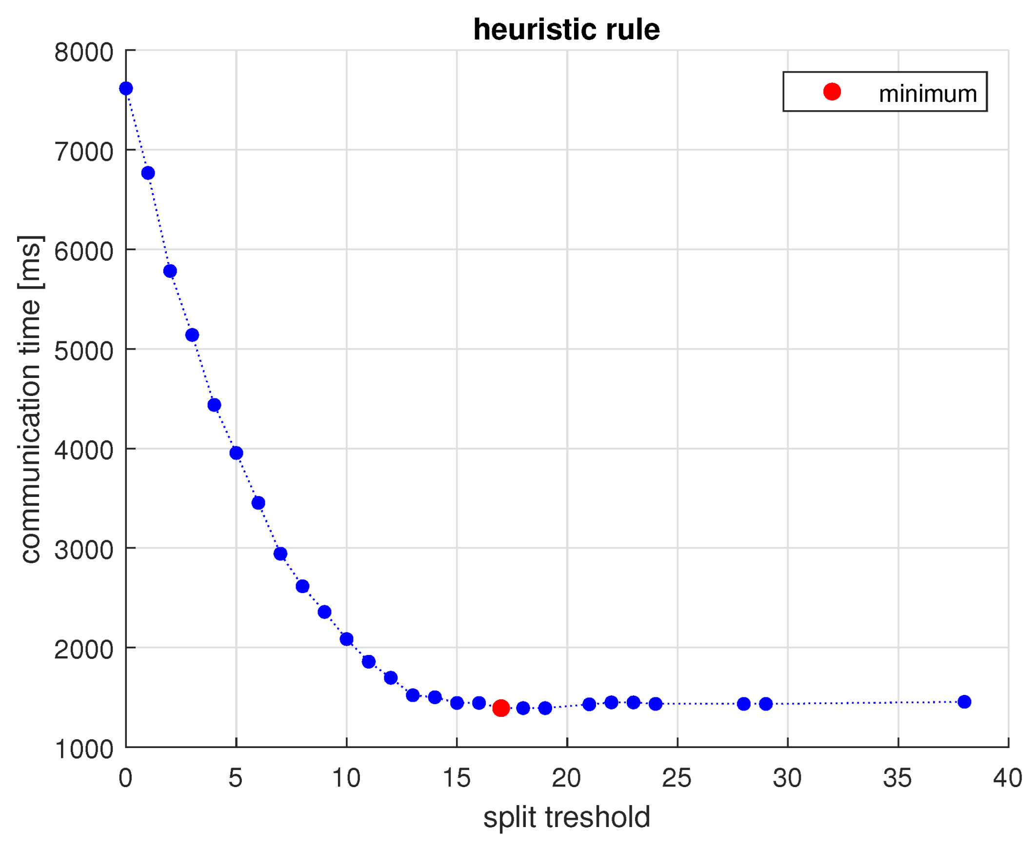
Algorithm 4: Pseudocode of algorithm HR

5. Experimental Verification

5.1. Benchmark Instances

For computational experiments, six sets of benchmark instances were generated, each of which having 10 instances. The instance parameters are based on the realistic case of the Modbus RTU protocol. For this communication, a baud rate $\nu$ in bits per second is defined. The logical unit of data is a byte that is physically transmitted as 9 bits; thus, its transmission time is $t_b=9000/\nu \mathrm{ms}$. The Modbus RTU register consists of 2 bytes. One register can be transferred in an individual transaction with total frame headers of 14 bytes using the FC6 protocol function. Another function (FC16) makes it possible to transmit multiple registers in one transaction; then, the headers have 17 bytes. The frames of any transaction have to be separated by pauses of time $7t_b$. We assume also that any transaction requires additional time $t_p=20\mathrm{ms}$ for data processing on the transmitter and receiver sides. According to this information, as the description of the problem $\mathcal{P}=\left(R,s,\mu ,\alpha ,\beta \right)$ one obtains

$$\begin{array}{cc}\hfill & \mu =2t_b+14t_b+7t_b+t_p=207,000/\nu +20,\hfill \\ \hfill & \alpha =2t_b=18,000/\nu ,\hfill \\ \hfill & \beta =17t_b+7t_b+t_p=216,000/\nu +20,\hfill \end{array}$$

where the time unit is a millisecond.

The maximum Modbus RTU frame size is 255 bytes. The header of the output frame of the FC16 function has 9 bytes. Therefore, the parameter s of $\mathcal{P}$ must satisfy the equation $9+2s=255$, resulting in $s=123$.

In this way, all the parameters of the problem needed for computations are established. Experiments have been conducted for five standard Modbus baud rates, namely $\nu \in \{9600;19,200;38,400;57,600;115,200\}$.

5.2. Optimization Tools

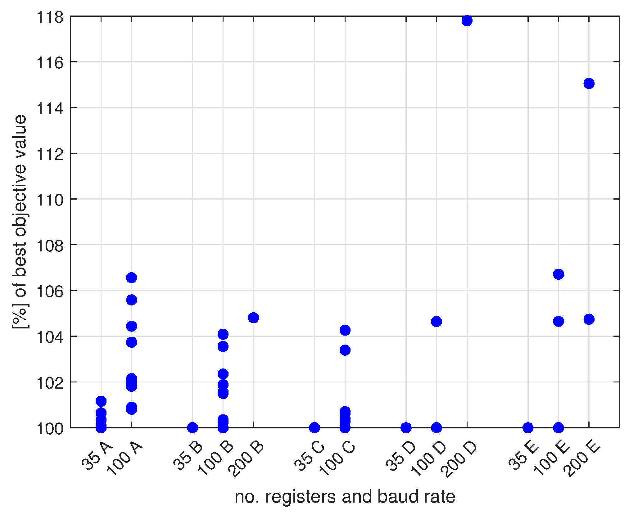
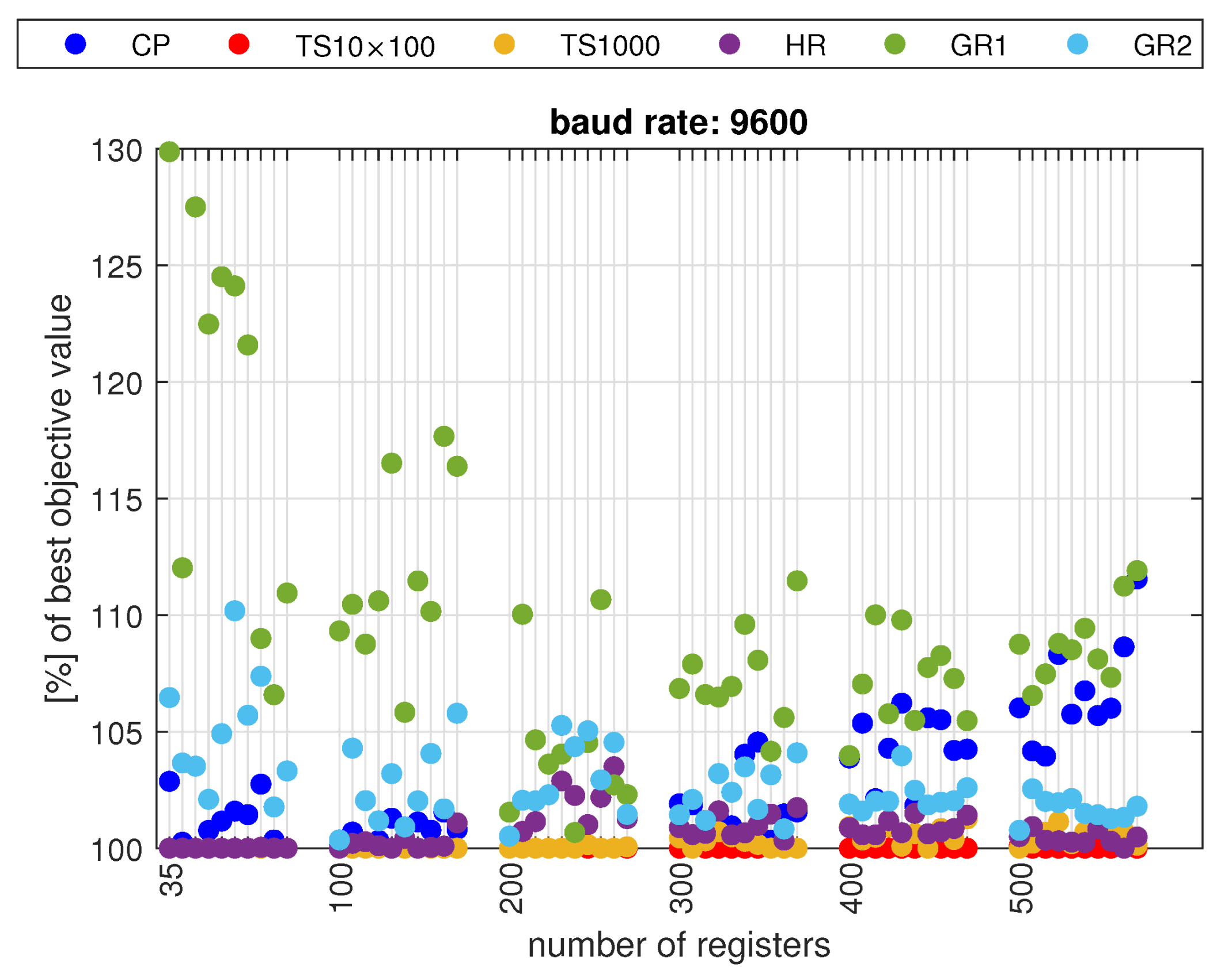
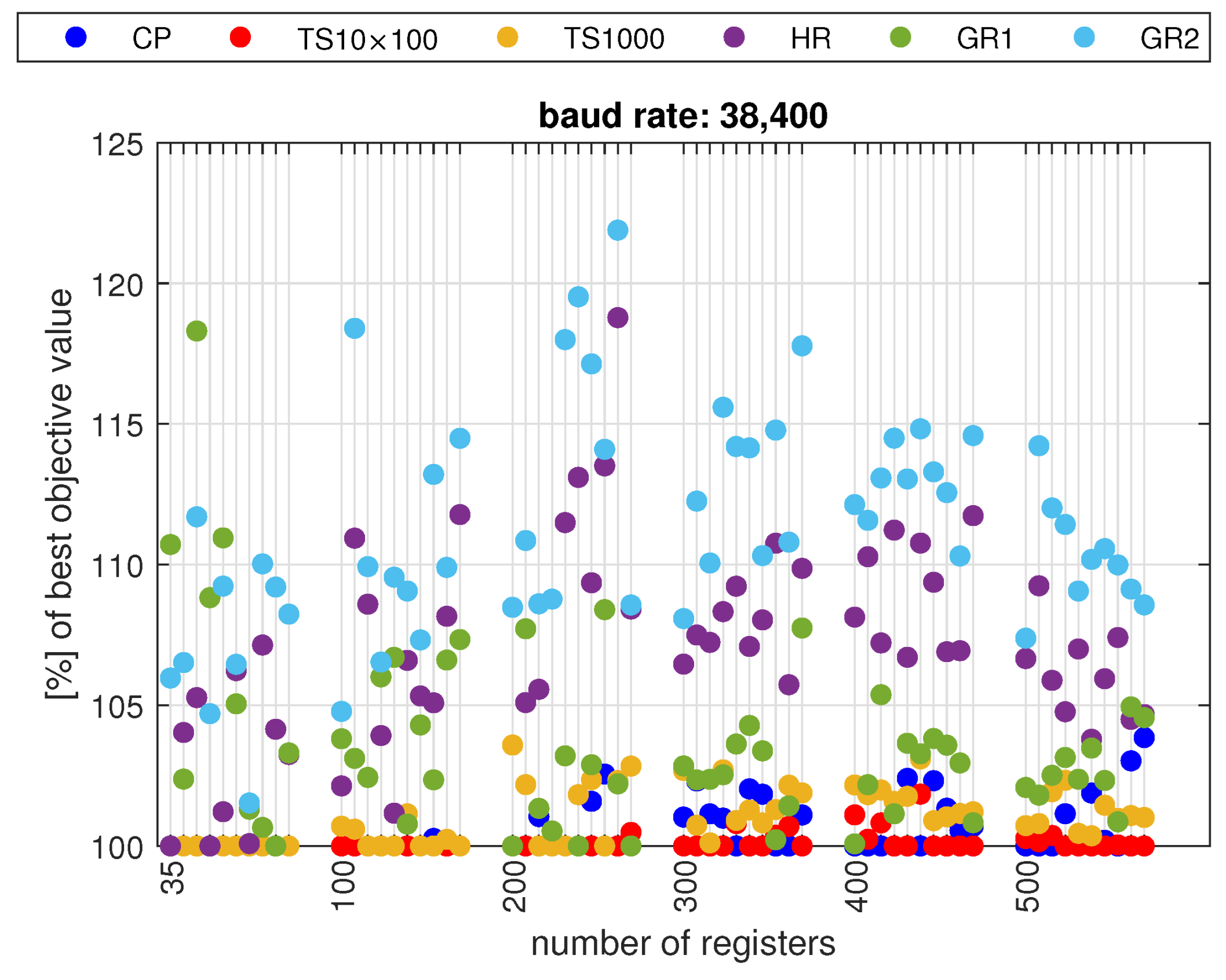
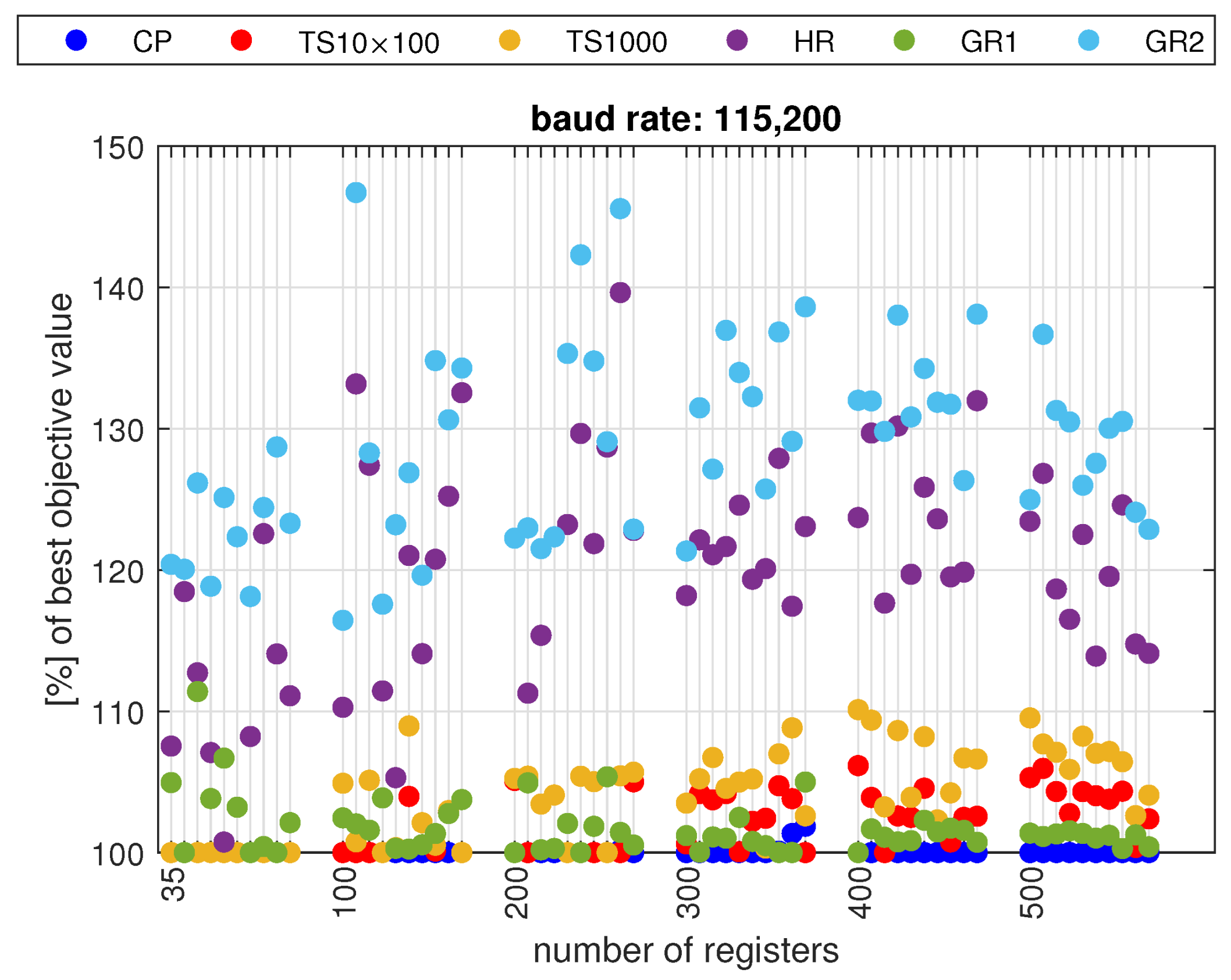
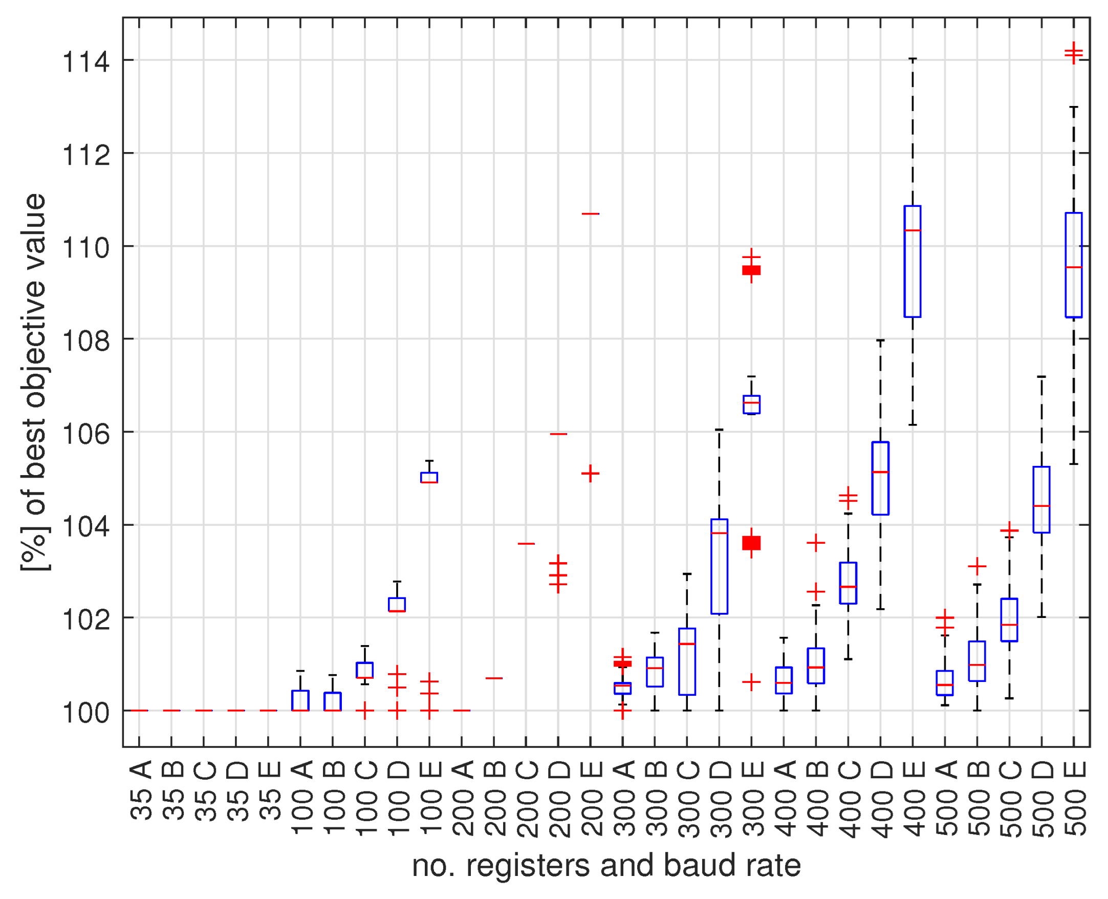
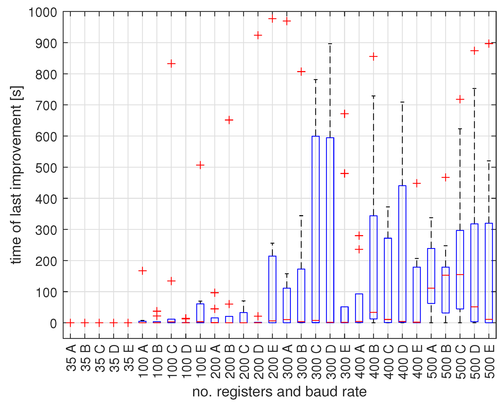
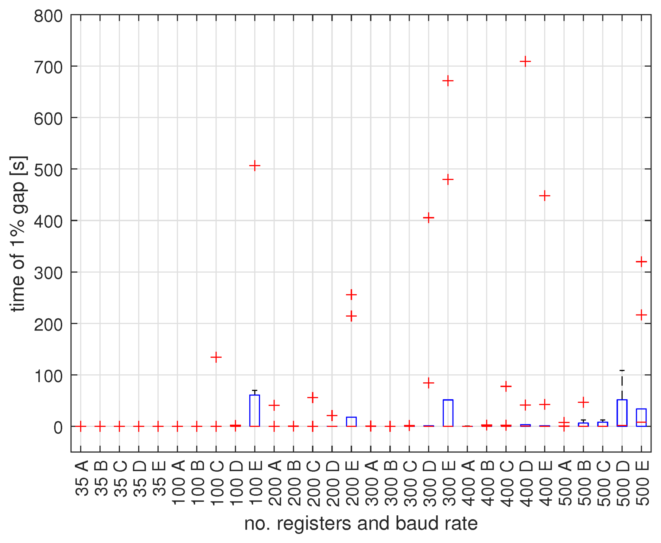
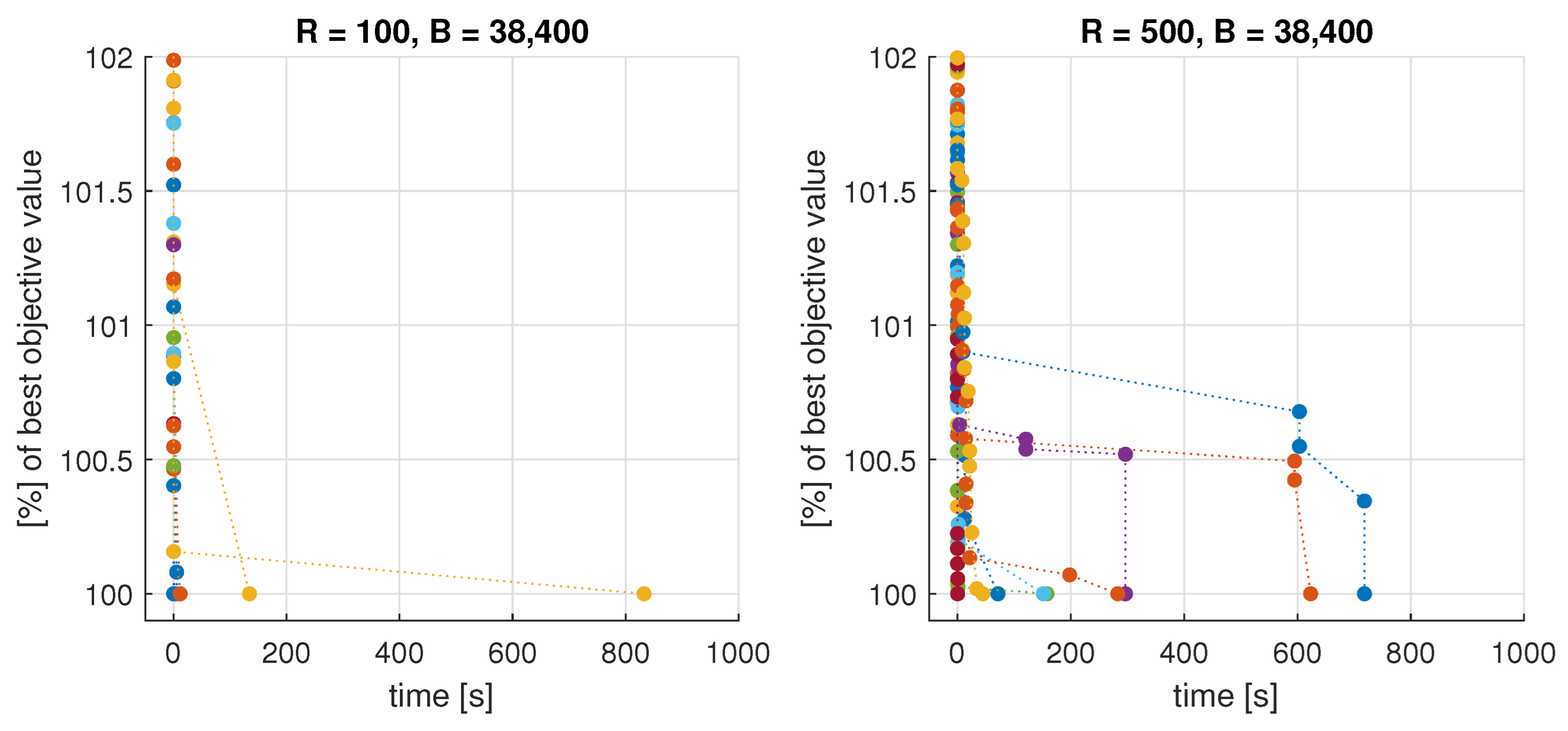
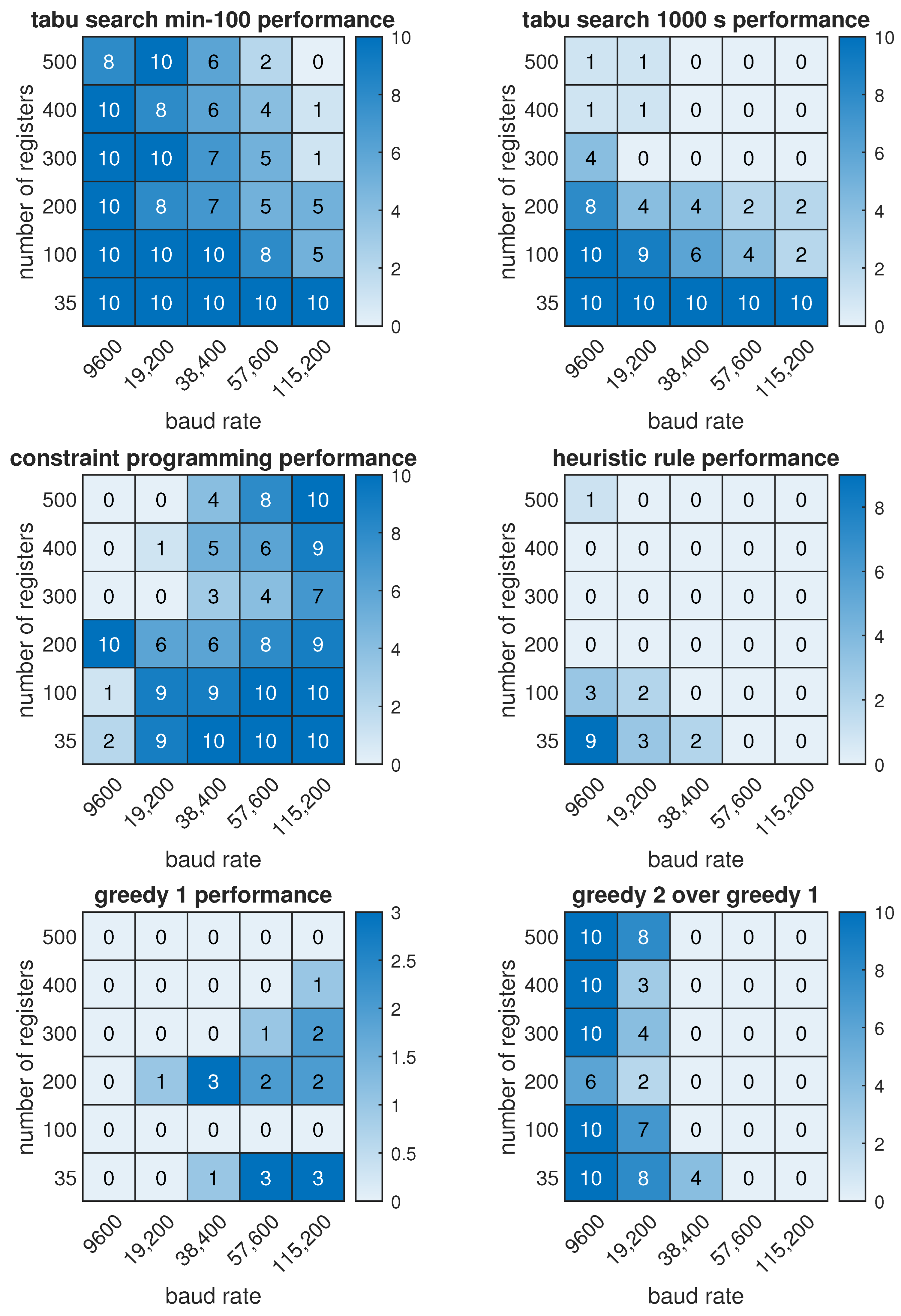
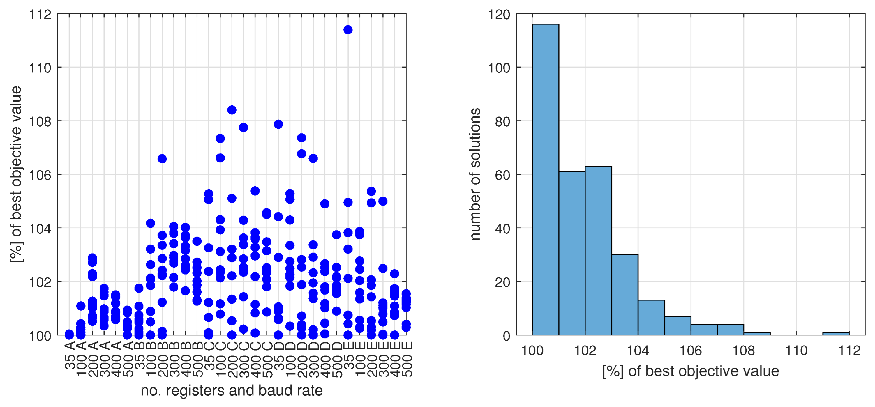
The MILP and constraint programming models were implemented and solved using IBM CPLEX Optimization Studio [23,24]. The remaining algorithms were coded directly in the Java programming language. All computations were performed using a machine with Ryzen 9 3900X 12-Core processor (AMD, Santa Clara, CA, USA) and 96 GB RAM. The IBM CPLEX Optimization Studio solvers used multithreading to increase performance, whereas other algorithms run in a single thread. The MILP and constraint programming optimization were run with a 1000 s time limit for each benchmark instance. The tabu search was run in two configurations for each instance: (a) once for 1000 s and (b) 100 times for 10 s. The tabu search was also run with an inverted optimization direction (maximization of the objective function) to estimate the worst possible result for comparison. The tabu search parameters were set to $p^{\mathrm{TS}}=0.5$ and $l^{\mathrm{TS}}={10}^4$. The deterministic algorithms are executed almost instantly for the considered benchmarks; thus, the time limits are irrelevant for them.

5.3. Results

The practical usefulness of an exhaustive search ends at instances of 30…40 registers, due to the computation time. Among other methods, the MILP and CP optimization can provide proofs of optimality (the equality of lower and upper bounds of the objective function), but this was not achieved in the tested cases. For this reason, a relative comparison of the results was used, related to the smallest value of the objective function obtained by any of the methods for a given instance (unless otherwise stated). This is how the term “[%] of best objective value” should be understood. The exception is the case of 35 registers, where the reference value is the optimal result obtained from the exhaustive search.

For the sake of brevity, in the descriptions of the graphs containing both the number of registers and the transmission speed, this speed has been abbreviated with the letters A–E for the baudrates 9600 to 115,200 bps, respectively.

Figure 3 shows the results obtained by the MILP, taking into account only the objective function values below 140% of the best value, in order to improve readability. For the smallest number of registers equal to 35, the results are favorable, practically identical to the optimum (B–E) or close (A). For 100 registers, the objective function values deviate from the best, but not more than 10%. For 200 registers, the results diverge dramatically (many not visible in Figure 3), and for some of the instances, no result was obtained within the 1000 s time limit. For instances with 300 or more registers, the MILP method never provided any result within the time limit. The results indicate that the MILP application is characterized by a high computational complexity and poor scalability with the number of registers. This is the only method for which such a problem has been found; therefore, it will be omitted from further listings as it is inadequate for the considered task.

Comparison of the results of all methods except MILP is shown in Figure 4, Figure 5 and Figure 6, sequentially for each baud rate. The TS10×100_min points represent the best (smallest) value of the objective function from 100 repetitions of a 10-s run of the TS algorithm for a given instance. All other algorithms were run once, and marked points directly indicate their results. Comparison of the graphs in Figure 4, Figure 5 and Figure 6 shows that the relations between the effectiveness of individual methods change as a function of the number of registers, but also clearly as a function of the baud rate. This suggests the need for a closer analysis of these dependencies, which will be conducted in the following paragraphs.

In Figure 7, a summary of the communication times obtained for an example instance (registers: 300, baudrate: 38,400 bps) is presented. Six optimization results are taken into account, including the distribution of 100 repetitions of TS. These minimization results were supplemented with the distribution of 10,000 results based on the random grouping of registers and the maximum communication time value determined by the TS algorithm. It can be observed that the minimization results, although varied, represent a narrow range of values compared to the communication time of random clustering, and even more so compared to the pessimistic solution. This indicates that without a dedicated optimization process, one cannot count on a good result, and each of the proposed methods provides a much better effect than a random grouping or even the best result from a large number of such random groupings. For all other instances examined, the distribution of values is similar to the one presented in Figure 7.

In Figure 8, Figure 9, Figure 10 and Figure 11, the results of the TS algorithm are shown. The distribution of the relative values of the objective function is shown in the box plot in Figure 8. For each combination of the number of registers and transfer speed, 100 repetitions of the algorithm, 10 s each, were performed for the first of 10 test instances. The graph shows that for 35 registers, the algorithm reliably provides the optimal solution in each execution. There is also a trend of an increase in the deviation from the best value with the increase in the number of registers and for a fixed number of registers with the increase in the transmission speed. However, only in two cases (200 E, 400 E) does the median exceed 110%, while no result exceeds 115%. To test whether it is worth extending the work time of the TS algorithm, the times of the last improvement of the result for the algorithm running for 1000 s were determined. The distribution of the times obtained for the sets of all 10 instances is shown in the box plot in Figure 9. In the case of 35 registers, the last improvement leading to the optimal value (compare Figure 8) occurs practically immediately. As the number of registers and transmission speed increases, it takes longer and longer to improve the objective function, and the last updates also occur just before the timeout (1000 s), although the median never exceeds 3 min. However, late improvement in the objective function is rare, which is confirmed by Figure 10, which shows the distribution of times when the objective function value is below 101% for the first time. Exemplary TS algorithm convergence graphs for instances differing in the number of registers (100 vs. 500) are shown in Figure 11. Subsequent results obtained by TS instances are marked with dots of the same color, connected by a dashed line. Different colors represent distinct TS instances started from random initial solutions. Values above 102% have been omitted for readability. The graph shows that the objective function reaches approximately 101% almost immediately, i.e., 1% above the final value, and only further improvement requires a longer time, especially for a large number of registers.

For the selected test instance, the dependence of the objective function in the heuristic method on the register division threshold is shown in Figure 12. When the threshold is small, there are too often divisions into separately transmitted groups, which significantly extends the communication time. However, when the threshold is too large, additional divisions occur due to the frame size limitation that is not necessarily located in the largest gaps between registers, and also slightly worsens the solution. As expected, the minimum is between the extreme thresholds of the division. An analogous regularity occurs for all other examined instances of the problem.

Since the results presented in Figure 4, Figure 5 and Figure 6 do not indicate a clear advantage of any particular method, they were additionally compared using the matrices shown in Figure 13. All matrices, except for the last one, specify for how many out of 10 instances a given method provided the best results. The most effective for the adopted comparative criterion turned out to be the TS algorithm performed 100 times for 10 s. In particular, it can be observed that such a multiple start is much more advantageous than one continuous TS execution in the equivalent time of 1000 s for cases with a large number of registers and a high transfer rate. Simple deterministic algorithms (HR, GR1, GR2) turned out to be weaker for the adopted criterion. In particular, GR2 did not provide the best solution for any of the instances. For this reason, in order to omit the trivial plot, the last matrix contains a comparison of GR1 and GR2 by indicating the number of instances for which GR2 was better than GR1. It turns out that GR2 gives better results than GR1 for cases with a slow transfer rate.

The poor performance of the deterministic algorithms leads to the question whether such algorithms would be useful in practice. Certainly, they are relatively ineffective in obtaining the best solutions that are as close as possible to the global optimum. However, if the deviation from the best results of other methods is not too big, maybe it is worth using them due to the simple implementation and very fast operation. It is worth asking whether the result will be satisfactory if all three algorithms (HR, GR1, GR2) are implemented and executed, and then the best of the three results is selected. The answer is indicated by the graphs in Figure 14, showing the distribution by the number of registers and transfer rate (left), and the histogram distribution (right) for the result which is the minimum of the objective function values obtained by HR, GR1 and GR2. In most cases, the result does not exceed the minimum value by 5%, which in practice may be sufficient.

6. Conclusions

The problem of communication time minimization in industrial automation systems has been considered in this work. The proposed solutions are intended for systems with the register-based data transfer, which is characteristic of many fieldbus networks. In this form of communication, each register can be transferred, either separately or in a larger continuous block. In the former case, there is a relatively large overhead of a frame size (header, address, etc.) compared to the raw register transfer time. In the latter case, redundant registers from the continuous block have to be transferred, wasting transmission time. It is an optimization problem to determine a partition into separate registers and their blocks, which minimizes the total communication time. According to related works, this problem has not been considered so far, except for in much simpler cases, e.g., with only two groups of registers. In this study, a general form of the register-based data transfer has been formulated, and a comprehensive set of optimization approaches has been developed and tested.

Much work was applied to validate the results obtained. A multilevel internal validation was applied. On the lowest level, small problem instances (like the one in Figure 1) were solved both by hand and by the algorithms, and equivalency was confirmed. Then, the results of an exhaustive search were successfully confronted with the results of other methods; in particular, the TS and CP methods typically find the global optimum for the instances with 35 registers, as expected. Finally, the results of all the approaches are consistent even for large problem instances (see e.g., Figure 7). There is also one negative finding of the validation; namely, we discovered the MILP-based optimization to be highly inefficient in our problem. A separate thread concerns the formulation of the fast optimization procedure for specific problem parameters, where the validity is based on mathematical rigor. The external validity is mainly based on two pillars. First, the addressed Modbus RTU protocol is deterministic; thus, the real-world communication timing has to conform to the results of the calculations. Second, the problem formulation assumes a flexible parameterization; thus, it is adaptable to virtually any Modbus configuration (baud rate, serial port settings, and interframe gap) and also to other protocols with the register-based data transfer.

The computational complexity of the problem was taken into account. The introduction of binary solution encoding revealed that a dedicated exhaustive search algorithm has a time complexity of the order $O\left(2^n\right)$, where $n=\left|R\right|$. Therefore, this algorithm cannot be useful for larger problem instances, but we have experimentally checked that it may be sufficient if the number of registers does not exceed 35…40. We have also isolated a special easy case under conditions $\mu =\alpha +\beta$ and $s=\infty$, for which a linear time exact algorithm exists. Theorem 1 specifies details of this case along with the related solving procedure. However, the most attention was devoted to a general case for which we cannot find any fast and exact algorithm. Several approaches that were well suited for hard optimization problems were implemented and examined: MILP (mixed integer linear programming), CP (constraint programming), TS (tabu search), and three rule-based deterministic algorithms (GR1, GR2, HR). The methods based on MILP, CP, and TS are guided by the global objective function; however, their divergence may be too slow in practice. On the other hand, the algorithms GR1, GR2, and HR use local optima for decision making, and they may be less exact but work much faster. Therefore, we have performed extensive experimental verification and comparison of the approaches.

The practical usefulness of the considered problem solutions are supported by the observation that the total communication time can significantly depend on the partition of the registers. For instance, the minimized objective function value is many times less than for the randomly generated partitions in the case presented in Figure 7. As a result of the research, on the one hand, a practitioner obtains models and tools for an off-line communication analysis, as well as fast algorithms that are implementable on industrial controllers, on the other hand. We have not found a universal algorithm that always provides the best result in the shortest time. The practical guidelines explaining the applicability and limitations of the examined optimization approaches are as follows:

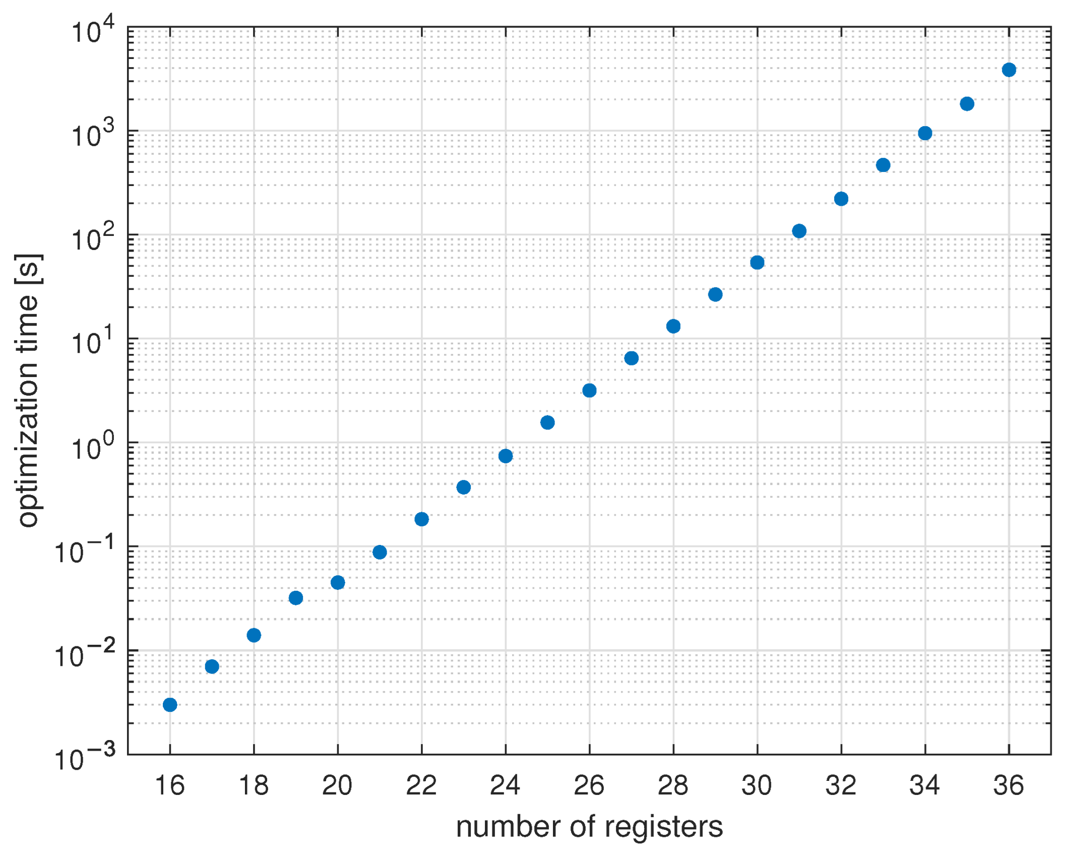
• The exhaustive search algorithm can be practically useful, but only for problems with up to 30…40 registers;
• An optimal solution can be constructed by a simple linear time algorithm described in the statement of Theorem 1, if the parameters of a problem instance meet the conditions $\mu =\alpha +\beta$ and $s=\infty$;
• MILP is ineffective for the considered problem. For a large number of registers, it is unable to find a solution in a reasonable time;
• The constraint programming (CP) provides better results for high transmission speeds, and the tabu search (TS) for low transmission speeds;
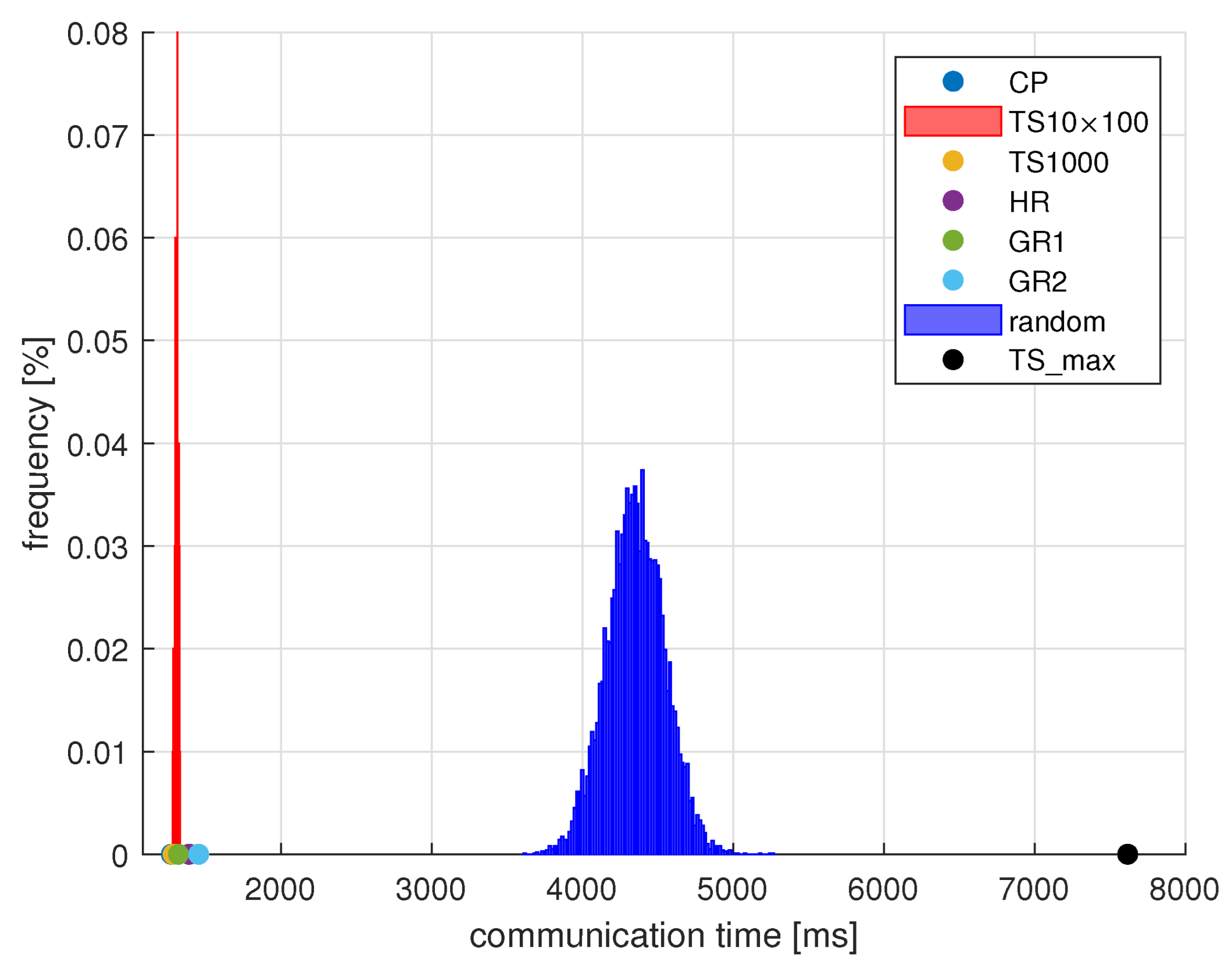
• It is more beneficial to run TS multiple times for a short time, with different random initial values, than to run it once for a longer time;
• CP and TS algorithms require significant computing power. They can be run on a PC, but not on a PLC;
• The proposed deterministic algorithms (greedy or heuristic) provide slightly worse results than CP and TS, but they require little computing power, so they can be implemented on a PLC;
• In some applications, the ability to quickly find a suboptimal solution on the PLC, which is slightly worse than the unknown optimal solution, will be sufficient.

We identify a few directions for future work. New optimization approaches can be developed, and research can be more focused on specific groups of approaches, e.g., nature-inspired algorithms or approximation algorithms. The implementation of the proposed algorithms in industrial controllers and their verification in real-world conditions is another direction. One can also extend the formulation of the problem considered in this work by additional elements that are important in practice.

References

1. Silva, M.; Pereira, F.; Soares, F.; Leão, C.P.; Machado, J.; Carvalho, V. An Overview of Industrial Communication Networks. In Proceedings of the New Trends in Mechanism and Machine Science; Flores, P., Viadero, F., Eds.; Springer: Cham, Switzerland, 2015; pp. 933–940. [Google Scholar]
2. Thomesse, J. Fieldbus Technology in Industrial Automation. Proc. IEEE 2005, 93, 1073–1101. [Google Scholar] [CrossRef]
3. Gaj, P.; Jasperneite, J.; Felser, M. Computer Communication Within Industrial Distributed Environment—A Survey. IEEE Trans. Ind. Inform. 2013, 9, 182–189. [Google Scholar] [CrossRef]
4. IEC 61158; Industrial Communication Networks—Fieldbus Specifications. IEC: Geneva, Switzerland, 2007.
5. Scanzio, S.; Wisniewski, L.; Gaj, P. Heterogeneous and dependable networks in industry—A survey. Comput. Ind. 2021, 125, 103388. [Google Scholar] [CrossRef]
6. Titaev, A. Reducing update data time for exchange via MODBUS TCP protocol by controlling a frame length. Autom. Control Comput. Sci. 2017, 51, 357–365. [Google Scholar] [CrossRef]
7. Rzonca, D. Performance Improvement of PLC—HMI Communication in CPDev Engineering Environment. Pomiary Autom. Robot. 2020, 24, 35–40. [Google Scholar] [CrossRef]
8. Rzonca, D. Acceleration of Modbus Data Exchange between PLC and HMI Using the CPDev Engineering Environment. Pomiary Autom. Robot. 2022, 26, 85–89. [Google Scholar] [CrossRef]
9. Găitan, V.G.; Zagan, I. Modbus Protocol Performance Analysis in a Variable Configuration of the Physical Fieldbus Architecture. IEEE Access 2022, 10, 123942–123955. [Google Scholar] [CrossRef]
10. Zagan, I.; Găitan, V.G. Enhancing the Modbus Communication Protocol to Minimize Acquisition Times Based on an STM32-Embedded Device. Mathematics 2022, 10, 4686. [Google Scholar] [CrossRef]
11. Găitan, V.G.; Zagan, I. Experimental Implementation and Performance Evaluation of an IoT Access Gateway for the Modbus Extension. Sensors 2021, 21, 246. [Google Scholar] [CrossRef] [PubMed]
12. Bednarek, M.; Będkowski, L.; Dąbrowski, T. The selected functions of supervision and therapeutic system in a communication system. Diagnostyka 2005, 34, 31–36. [Google Scholar]
13. Dutertre, B. Formal Modeling and Analysis of the Modbus Protocol. In Proceedings of the Critical Infrastructure Protection; Goetz, E., Shenoi, S., Eds.; Springer: Boston, MA, USA, 2008; pp. 189–204. [Google Scholar]
14. Twaróg, B.; Gomółka, Z.; Żesławska, E. Time Analysis of Data Exchange in Distributed Control Systems Based on Wireless Network Model. In Proceedings of the Analysis and Simulation of Electrical and Computer Systems; Mazur, D., Gołębiowski, M., Korkosz, M., Eds.; Springer: Cham, Switzerland, 2018; pp. 333–342. [Google Scholar] [CrossRef]
15. Künzel, G.; Corrêa Ribeiro, M.A.; Pereira, C.E. A Tool for Response Time and Schedulability Analysis in Modbus Serial Communications. In Proceedings of the 2014 12th IEEE International Conference on Industrial Informatics (INDIN), Porto, Portugal, 27–30 July 2014; pp. 446–451. [Google Scholar] [CrossRef]
16. Persechini, M.A.M.; Mendes, L.T.S. Performance analysis among different acquisition systems for process control. ISA Trans. 2020, 97, 86–92. [Google Scholar] [CrossRef]
17. Kim, B.; Lee, D.; Choi, T. Performance evaluation for Modbus/TCP using Network Simulator NS3. In Proceedings of the TENCON 2015–2015 IEEE Region 10 Conference, Macao, China, 1–4 November 2015; pp. 1–5. [Google Scholar] [CrossRef]
18. Robert, J.; Georges, J.P.; Rondeau, E.; Divoux, T. Minimum cycle time analysis of Ethernet-based real-time protocols. Int. J. Comput. Commun. Control 2012, 7, 743–757. [Google Scholar] [CrossRef]
19. Bożek, A.; Werner, F. Flexible job shop scheduling with lot streaming and sublot size optimisation. Int. J. Prod. Res. 2017, 56, 6391–6411. [Google Scholar] [CrossRef]
20. Bożek, A. Energy Cost-Efficient Task Positioning in Manufacturing Systems. Energies 2020, 13, 5034. [Google Scholar] [CrossRef]
21. Glover, F. Tabu Search—Part I. ORSA J. Comput. 1989, 1, 190–206. [Google Scholar] [CrossRef]
22. Glover, F.; Laguna, M.; Martí, R. Principles and Strategies of Tabu Search. In Handbook of Approximation Algorithms and Metaheuristics, 2nd ed.; Chapman and Hall/CRC: Boca Raton, FL, USA, 2018; pp. 361–377. [Google Scholar] [CrossRef]
23. Anand, R.; Aggarwal, D.; Kumar, V. A comparative analysis of optimization solvers. J. Stat. Manag. Syst. 2017, 20, 623–635. [Google Scholar] [CrossRef]
24. Laborie, P.; Rogerie, J.; Shaw, P.; Vilím, P. IBM ILOG CP optimizer for scheduling. Constraints 2018, 23, 210–250. [Google Scholar] [CrossRef]
Figure 1. Solutions of an exemplary problem instance with: (a) the worst, (b) intermediate, and (c) the best objective function value.
Electronics 12 04917 g001
Figure 2. Exhaustive search optimization time as a function of the number of registers.
Electronics 12 04917 g002
Figure 3. Results obtained by MILP optimization.
Electronics 12 04917 g003
Figure 4. Minimized communication times for B = 9600 .
Electronics 12 04917 g004
Figure 5. Minimized communication times for B = 38,400 .
Electronics 12 04917 g005
Figure 6. Minimized communication times for B = 115,200 .
Electronics 12 04917 g006
Figure 7. Communication time comparison for R = 300 , B = 38,400 .
Electronics 12 04917 g007
Figure 8. Best results obtained by tabu search (single instance).
Electronics 12 04917 g008
Figure 9. Time of last improvement achieved by tabu search.
Electronics 12 04917 g009
Figure 10. Time up to 1% gap of tabu search.
Electronics 12 04917 g010
Figure 11. Examples of tabu search progress.
Electronics 12 04917 g011
Figure 12. Communication time as a function of heuristic rule split threshold for R = 300 , B = 38,400.
Electronics 12 04917 g012
Figure 13. Performance comparison.
Electronics 12 04917 g013
Figure 14. Net performance of deterministic algorithms: HR, GR1, and GR2.
Electronics 12 04917 g014
Disclaimer/Publisher’s Note: The statements, opinions and data contained in all publications are solely those of the individual author(s) and contributor(s) and not of MDPI and/or the editor(s). MDPI and/or the editor(s) disclaim responsibility for any injury to people or property resulting from any ideas, methods, instructions or products referred to in the content.