Dynamical Analysis of a Memristive Chua’s Oscillator Circuit

Abstract

In this work, a novel memristive Chua’s oscillator circuit is presented. In the proposed circuit, a linear negative resistor, which is parallel coupled with a first-order memristive diode bridge, is used instead of the well-known Chua’s diode. Following this, an extensive theoretical and dynamical analysis of the circuit is conducted. This involves numerical computations of the system’s phase portraits, bifurcation diagrams, Lyapunov exponents, and continuation diagrams. A comprehensive comparison is made between the numerical simulations and the circuit’s simulations performed in Multisim. The analysis reveals a range of intriguing phenomena, including the route to chaos through a period-doubling sequence, antimonotonicity, and coexisting attractors, all of which are corroborated by the circuit’s simulation in Multisim.

1. Introduction

The exploration of chaos has captivated the research community since the late 19th century, sparked by Henry Poincaré’s groundbreaking observations in 1889 [1]. However, the formalization of chaos theory gained substantial momentum after the decade of the 1960s, driven by the examination of evolving physical systems [2,3]. Later, numerous researchers asserted that chaos manifests across diverse disciplines, encompassing chemistry, biology, economics, mechanics, and more [4,5,6,7,8,9].

Beginning in 1983, there was a notable upswing in the study of nonlinear dynamics and chaos by using electronic circuits, initiated by Chua’s design and implementation of the first autonomous chaotic electronic circuit [10,11,12,13]. However, the implementation of chaotic circuits was made possible by earlier advancements in the design and realization of nonlinear resistors with negative slopes, including the transitron, kallirotron, dynatron [14], and others [15,16], crucial elements in the design of these nonlinear circuits. The introduction of the transistor in 1947 prompted investigations into solid-state negative resistors [17]. In 1958, Esaki unveiled the tunnel diode, followed by the Gunn diode eight years later [18,19]. Nonetheless, the advent of operational amplifiers empowered scientists to effortlessly realize nonlinear electrical elements with current versus voltage piecewise-linear functions.

Esteemed as a paradigm, Chua’s circuit represents the pioneering chaotic circuit, systematically deriving chaos, undergoing physical validation and meticulous scrutiny [11,12]. To elaborate, for a span of three decades, Chua’s circuit remained the simplest chaotic circuit, encompassing merely five components: a resistor, an inductor, two capacitors, and a nonlinear element referred to as a Chua’s diode. The resistor, inductor, and capacitors are conventional components, while the design and implementation of the nonlinear element can vary, contingent upon its intended application. Later, with the inclusion of the minor ohmic resistance R_L of the inductor, the recognizable form of Chua’s oscillator circuit emerged.

The circuit’s implementation of Chua’s oscillator offers versatility, allowing for various approaches. Since all the linear components (resistors, capacitors, inductors) are commercially available, attention is directed toward realizing the nonlinear element. Initially, Chua designed Chua’s diode, as a standard voltage–current nonlinear circuit element, by connecting two negative impedance converters in parallel. Presently, diverse implementations utilizing operational amplifiers [20,21], diodes [22], transistors [23], and transconductance amplifiers [24] have been proposed.

Moreover, in 2007, researchers at Hewlett-Packard successfully developed a solid-state thin-film two-terminal memristor [25]. Four decades earlier, Leon Chua had also introduced the memristor as one more of the fundamental circuit elements, alongside the traditional trio of elements—the resistor, inductor, and capacitor. This fourth element is defined in terms of a nonlinear constitutive relation between two key circuit variables: charge and magnetic flux [26]. After this milestone, a considerable number of publications have showcased significant discoveries related to memristor models, fabricated materials, and techniques as well as substantial applications of memristors. These applications include adaptive filters [27], high-speed low-power processors [28], neural networks [29,30], associative memory [31,32,33], programmable analog integrated circuits [34] and more. It is noteworthy that the inherent nonlinear characteristic of memristors can be leveraged to devise innovative chaotic systems with intricate dynamics [35,36].

In this direction, the memristor can be used instead of Chua’s diode in the design of chaotic circuits. Therefore, derived from Chua’s circuit, Muthuswamy’s chaotic circuit was achieved by using a flux-controlled memristor instead of Chua’s diode [37]. Similar to this circuit, several other chaotic circuits based on memristors are devised by using, instead of the Chua’s diode, a memristor’s emulator characterized by smooth piecewise-quadratic nonlinearity [38], non-smooth piecewise linearity [35], or smooth cubic nonlinearity [39]. Also, in 2012, Buscarino et al. introduced a memristive Chua’s oscillator, in which two HP memristors are connected in anti-parallel, as its nonlinear resistor [40].

Furthermore, in 2014, Bao et al. introduced a first-order generalized memristor emulator, implemented by using a first-order memristive circuit featuring an RC filter and a parallel diode bridge [41]. This memristor emulator has been used, as a nonlinear resistor, in a variety of chaotic circuits [42,43,44,45]. Also, in 2021, Kengne et al. studied the dynamics of a generalized memristive diode-bridge-based jerk circuit, in which symmetry could be varied, and a plethora of nonlinear and complex behaviors were revealed [46]. These include the coexistence of symmetric and asymmetric attractors, coexisting symmetric and asymmetric bubbles of bifurcation, and symmetric and asymmetric double-scroll chaotic attractors. Also, in the same year, Xu et al. proposed a similar jerk circuit with the specific memristive diode-bridge emulator, in which asymmetric coexisting bifurcations and multi-stability phenomena were observed [47]. In 2022, Wu et al. used the aforementioned memristor emulator, in which a DC offset had been added to one of the branches of the memristive diode-bridge [48]. In this way, they observed that the symmetry of the two unstable index-2 saddle-foci equilibrium points had been broken, leading to the emergence of complex asymmetric kinetic behaviors with multi-stability in the proposed oscillator. Furthermore, in the same year, Ramadoss et al. studied the impact of a broken symmetry on the dynamics of the Shinriki oscillator. The broken symmetry was caused by the memristive diodes bridge with an asymmetric pinched hysteresis loop designed by selecting two pairs of semiconductor diodes with different electrical properties [49]. As a consequence of this broken symmetry, up to four coexisting asymmetric chaotic and periodic attractors are reported following changes in both initial conditions and parameters.

Additionally, this specific memristor emulator has been used instead of the Chua’s diode in the well-known canonical Chua’s circuit [50] and in a non-autonomous Chua’s circuit [51]. Also, in 2016, a novel memristive Chua’s circuit was proposed, which is constructed by connecting the generalized memristor emulator between a passive LC oscillator and an active RC filter [52]. This circuit has rich dynamical behavior, as it can generate hidden attractors and coexisting hidden attractors in a narrow parameter region. Moreover, in 2015, Chen et al. introduced a novel memristive chaotic circuit, formulated by using, instead of the nonlinear element in Chua’s circuit, the generalized memristor emulator of Bao et al. [53].

In this work, the Chua’s diode in a Chua’s oscillator circuit is replaced with the generalized memristor developed by Bao et al. [41], marking the first instance of such substitution. Considering the resistance R_L of the inductor in this particular circuit, in comparison to the simplified Chua’s circuit examined in [53], a different chaotic dynamical system with interesting phenomena is revealed. Additionally, it enables the examination of the impact of this parasitic resistance to the system’s behavior. Also, in this work, a different diode model, with a smaller saturation current, with regard to [50,51,52,53], has been used in order to investigate the circuit’s dynamics in other ranges of parameters. Finally, as mentioned, intriguing phenomena related to chaos theory have been exposed, including the route to chaos through the period-doubling sequence, the occurrence of antimonotonicity, and the manifestation of coexisting attractors.

The rest of the paper is structured as follows. In Section 2, the memristor’s emulator, as well as Chua’s oscillator circuit, which contains this nonlinear element, are presented. In Section 3, the 4-dimensional nonlinear dynamical system that describes the proposed circuit is investigated theoretically. Section 4 presents the comprehensive simulation results that elucidate the circuit’s behavior concerning various parameters. These results are derived from both the numerical integration of the dynamical system as well as the circuit’s simulation using Multisim. Lastly, Section 5 concludes the paper with summaries and reflections on potential avenues for future research.

2. The Memristive Chua’s Oscillator

This section presents in detail the memristive Chua’s oscillator circuit. The memristor’s emulator, which is based on a parallel RC filter with a diode bridge, is presented and its behavior is studied through Multisim simulations. Furthermore, the proposed circuit is presented, in which the aforementioned memristor’s emulator that is connected in parallel to a negative resistor has been used instead of the Chua’s diode.

2.1. The Memristor’s Emulator

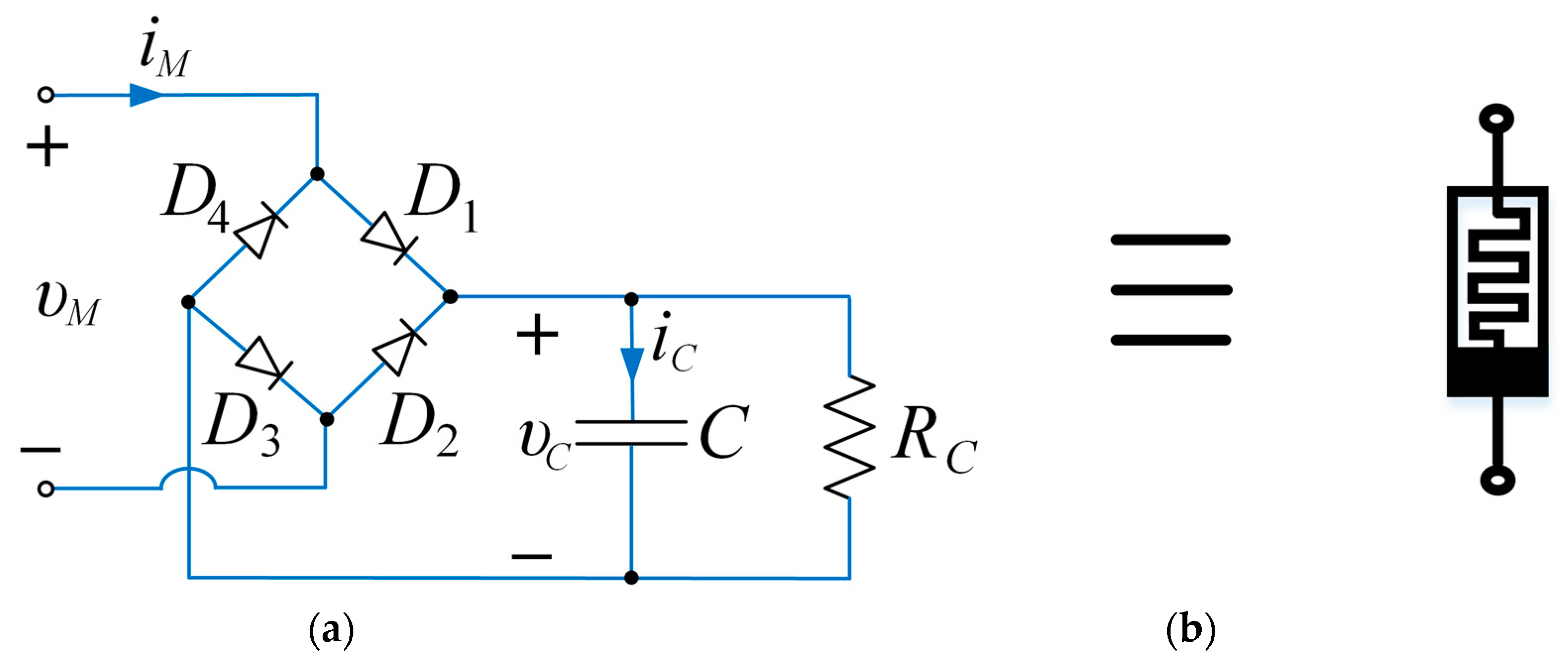
In the proposed circuit, the generalized memristor, which has been presented by Bao et al., is used [41]. A memristor emulator of this kind is composed of a first-order parallel RC filter with a diode bridge, illustrated in Figure 1, and is mathematically represented by the following set of equations:

$$i_M=G\left({\upsilon }_C,{\upsilon }_{{\rm M}}\right){\upsilon }_{{\rm M}}=2{{\rm I}}_S{e}^{-\rho {\upsilon }_C}\sin \mathrm{h}\left(\rho {\upsilon }_{{\rm M}}\right),$$

(1)

$$\frac{d{\upsilon }_C}{dt}=\frac{2{{\rm I}}_S\left[e^{-\rho {\upsilon }_C}\cosh \left(\rho {\upsilon }_{{\rm M}}\right)-1\right]}{C}-\frac{{\upsilon }_C}{R_{C}C},$$

(2)

where $i_M$ and ${\upsilon }_{{\rm M}}$ are the flowing current and the input voltage of the memristor’s emulator, and ${\upsilon }_C$ is the state variable corresponding to the voltage of the capacitor C. Furthermore, $\rho =1/\left(2n{V}_T\right)$, while the parameters $n$, $V_T$, ${{\rm I}}_S$ represent the emission coefficient, the thermal voltage, and the reverse saturation current of the diodes that have been used. Also, the memristor’s emulator, which is described by Equations (1) and (2), is a member of the family of extended memristors, based on the definition that Chua was given in [54]. According to this definition, any memristor can be considered as an extended memristor, if it can be described as follows:

$$\frac{d\mathit{x}}{ dt}=\mathit{F}\left(\mathit{x},\upsilon \right),$$

(3)

$$i_M=G\left(\mathit{x},\upsilon \right){\upsilon }_{{\rm M}},$$

(4)

where $\mathit{x}$ is, in general, the n-order state vector, $\mathit{F}$ is the state function, and $G$ is the memductance function, respectively. In the case of the memristor’s emulator of Equations (1) and (2), the memductance is as follows:

$$G=\frac{i_M}{{\upsilon }_{{\rm M}}}=\frac{2{{\rm I}}_S{e}^{-\rho {\upsilon }_C}sinh\left(\rho {\upsilon }_{{\rm M}}\right)}{{\upsilon }_{{\rm M}}}$$

(5)

Therefore, it is a voltage-controlled memristor. In

Table 1. The memristor’s emulator parameters.

Parameters	Significations	Values
${{\rm I}}_S$	Saturation current of 1N4149 diode	0.1 pA
$V_T$	Thermal voltage of 1N4149 diode	27 mV
n	Emission coefficient of 1N4149 diode	1
C	Capacitance	1 μF
RC	Resistance	500 Ω

, the memristor’s emulator parameters are listed.

When sinusoidal voltage stimuli are applied, the proposed memristor’s emulator displays the three distinctive features essential for identifying memristors [54]. Figure 2 depicts the Multisim-simulated pinched hysteresis loops of the proposed memristor for various values of frequencies (Figure 2a) and amplitudes (Figure 2b) of the sinusoidal voltage stimulus.

2.2. The Proposed Circuit

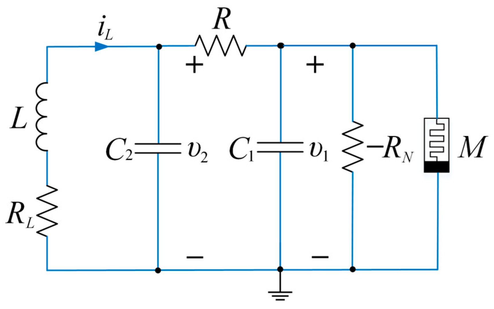
The proposed memristive circuit consists of two capacitors (C₁ and C₂) coupled via a linear resistor R, a parallel branch in the capacitor C₂, which has an inductor L, which is connected in series with a small resistor R_L and the nonlinear element that is connected in parallel to the capacitor C₁. In this work, the memristor’s emulator consisting of the first-order parallel RC filter with the diode bridge, which is connected in parallel with a linear negative resistor −R_N, has been used as the nonlinear element. Thus, Figure 3 depicts the proposed memristive circuit, and its parameters are outlined in

Table 2. The circuit’s parameters.

Parameters	Significations	Values
$L$	Inductance	15 mH
$C_1$	Capacitance	8 nF
$C_2$	Capacitance	Variable
R	Resistance	Variable
$R_L$	Resistance	10 Ω
$R_N$ = $R_3$	Linear resistance of the NIC	1400 Ω
$R_1$ = $R_2$	Other resistances of the NIC	1000 Ω
VS	Voltage Supply	±15 V

.

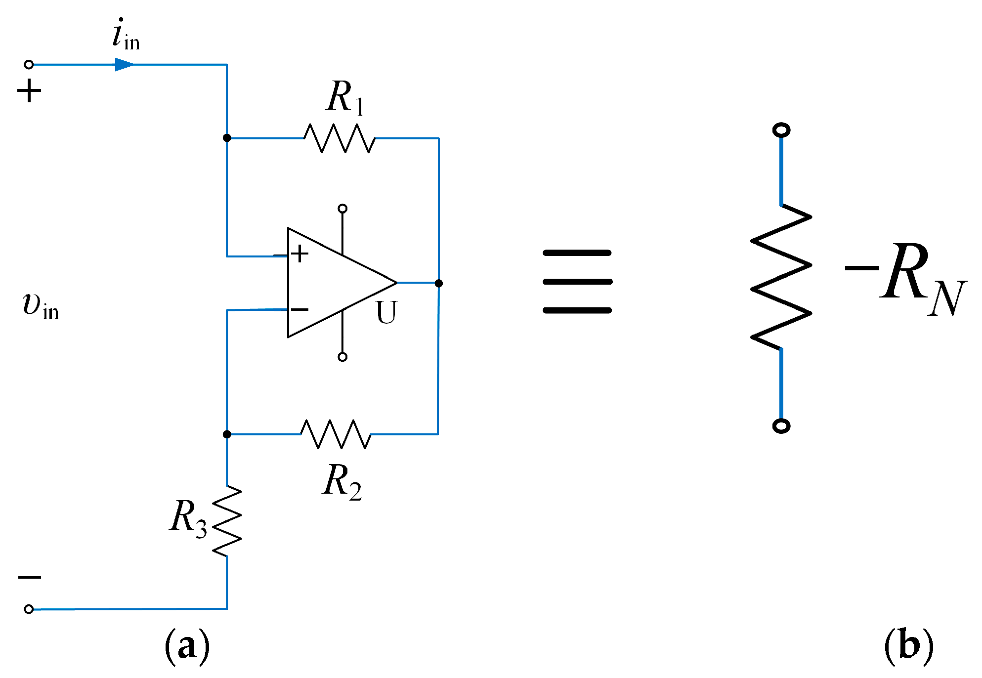
The negative resistor −R_N is realized using an op-amp-based negative impedance converter (NIC), as depicted in Figure 4. The linear negative resistance of this NIC is determined by solving the following equation:

$$\frac{{\upsilon }_{\mathrm{in}}}{i_{\mathrm{in}}}=\frac{-R_1{R}_3}{R_2}$$

(6)

When $R_1$ = $R_2$, the NIC circuit can be used as a negative resistance, with −R_N = −R₃.

For the simulation of the circuit in Multisim, the UA741 operational amplifier has been chosen.

By solving the circuit of Figure 3 with the use of Kirchhoff’s laws and the mathematical relationship of the memristor’s emulator described by Equations (1) and (2), the following system of differential equations is derived:

$$\left\{\begin{array}{c}{C}_1\frac{d{\upsilon }_1}{dt}=\frac{{\upsilon }_2-{\upsilon }_1}{R}+\frac{{\upsilon }_1}{R_N}-2I_S{e}^{-\rho {\upsilon }_C}\sinh \left(\rho {\upsilon }_1\right)\\ C_2\frac{d{\upsilon }_2}{dt}=i_L-\frac{{\upsilon }_2-{\upsilon }_1}{R}\\ L\frac{d{i}_L}{dt}=-{\upsilon }_2-R_L{i}_L\\ C\frac{d{\upsilon }_C}{dt}=2I_S\left[e^{-\rho {\upsilon }_C}\cosh \left(\rho {\upsilon }_1\right)-1\right]-\frac{{\upsilon }_C}{R_C}\end{array}\right.$$

(7)

where ${\upsilon }_1$, ${\upsilon }_2$, and ${\upsilon }_C$ are the voltages across the capacitors $C_1$, $C_2$, $C$, while $i_L$ is the current flowing through the inductor $L$.

By setting as $x=\rho {\upsilon }_1$, $y=\rho {\upsilon }_2$, $z=\rho r{i}_L$, $w=\rho {\upsilon }_C$, $a=\frac{r}{R}$,$b=2\rho r{I}_S$, $c=\frac{R_L}{r}$, $d=\frac{C_1}{C_2}$, $e=\frac{r}{R_C}$, $f=\frac{r}{R_N}$, $h=\frac{C_1}{C}$, $r=\sqrt{\frac{L}{C_1}}$, and $\tau =t/\sqrt{L{C}_1}$, the following system (8) in normalized form is derived:

$$\left\{\begin{array}{c}\frac{dx}{d\tau }=a\left(y-x\right)+fx-b{e}^{-w}\sinh \left(x\right)\\ \frac{dy}{d\tau }=d\left[z-a\left(y-x\right)\right]\\ \frac{dz}{d\tau }=-y-cz\\ \frac{dw}{d\tau }=h\left\{b\left[e^{-w}\cosh \left(x\right)-1\right]-ew\right\}\end{array}\right.$$

(8)

3. Theoretical Analysis

The theoretical analysis of the nonlinear dynamical system, which is described by system (8), is presented in this section.

3.1. Dissipativity Analysis

The memristive Chua’s oscillator circuit of Figure 3 exhibits dissipative behavior within certain parameter ranges. This dissipative nature can be deduced from the following:

$$\nabla V=\frac{\partial \dot{x}}{\partial x}+\frac{\partial \dot{y}}{\partial y}+\frac{\partial \dot{z}}{\partial z}+\frac{\partial \dot{w}}{\partial w}=-2a-e-c+f-b\left(h+1\right)e^{-w}coshx$$

(9)

Given that the hyperbolic cosine and the exponential function are both positive, Equation (9) could be simplified as follows:

$$\nabla V\le -2a-e-c+f$$

(10)

Considering the circuit’s parameters outlined in Table 1 and Table 2, and by also using C₂ = 170 nF and R = 1450 Ω, it is observed that Equation (10) yields a negative value of $\nabla V\le -3.6565$. This implies that all trajectories within the system will be constrained to a certain subset with zero volume, and the asymptotic motion will converge toward an attractor [55].

3.2. Equilibrium Points

For the calculation of the equilibrium points of system (8), the circuit’s parameters are depicted, as in Table 1 and Table 2, while C₂ = 170 nF and R = 1450 Ω, so that the circuit is in a chaotic mode, as it will be presented in the next section.

The equilibrium points of system (8) are determined by solving the following set of equations:

$$\left\{\begin{array}{c}a\left(y-x\right)+fx-b{e}^{-w}\sinh \left(x\right)=0\\ d\left[z-a\left(y-x\right)\right]=0\\ -y-cz=0\\ h\left\{b\left[e^{-w}\cosh \left(x\right)-1\right]-ew\right\}=0\end{array}\right.$$

(11)

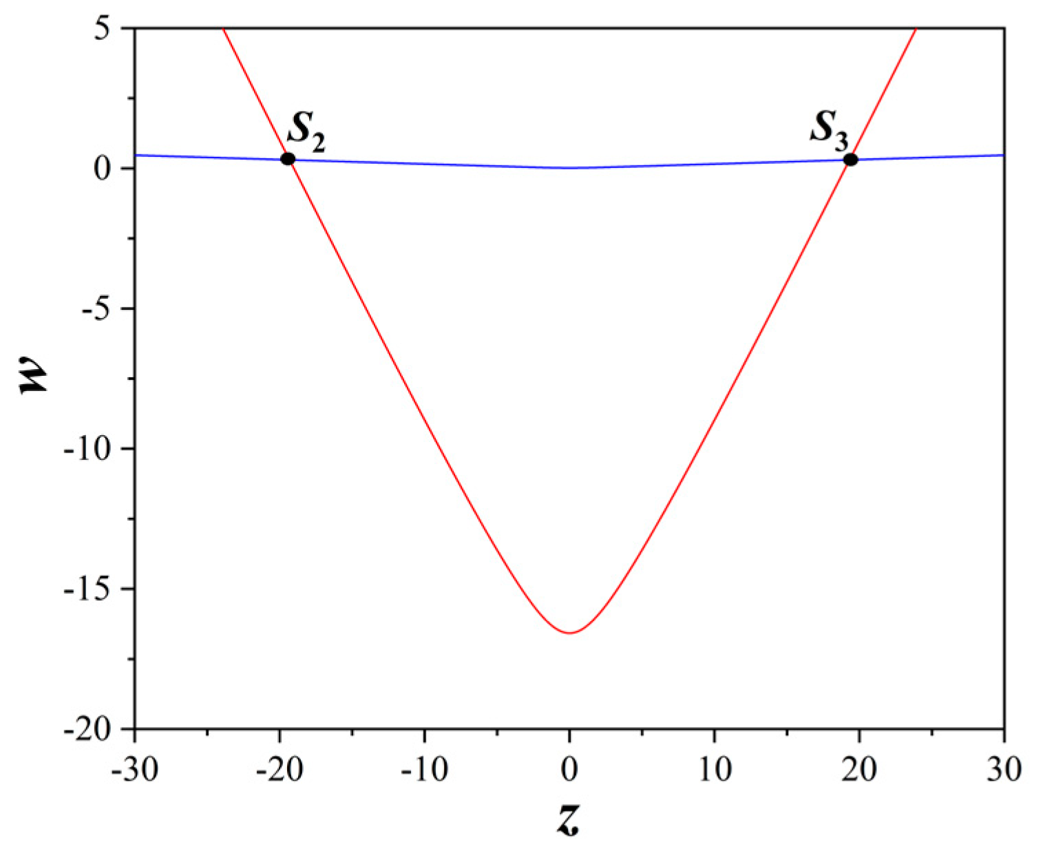
Therefore, the proposed system (8) has three equilibrium points. The first is the obvious solution of system (11), which is S₁ = (0, 0, 0, 0). The other two equilibrium points must be found graphically due to the fact that system (11) has two functions that describe the relation between the variables w and z, which are presented by Equations (12) and (13).

$$w=\frac{b}{e} \frac{\left(a-f-fac\right)z}{ab} \cot \mathrm{h}\left(-\frac{1+ac}{a}z\right)-\frac{b}{e}$$

(12)

$$w=\frac{\log \left(ab\sin \mathrm{h}\left(-\frac{1+ac}{a}z\right)\right)}{\left(a-f-fac\right)z}$$

(13)

In Figure 5, the graphical representation of the functions, which are described by the aforementioned Equations (12) and (13) are depicted in red and blue color respectively, as well as the intersection points that represent the two other equilibrium points S₂ = (19.86231, 0.13985, −18.61333, 0.29136) and S₃ = (−19.86231, −0.13985, 18.61333, 0.29136).

3.3. Stability

The first step in the procedure of finding the stability of system (8) is to find the Jacobian matrix described by Equation (14):

$$J=\left[\begin{array}{cccc}f-a-k_2& a& 0& k_1\\ ad& -ad& d& 0\\ 0& -1& -c& 0\\ bh{k}_1& 0& 0& -h\left(e+k_2\right)\end{array}\right]$$

(14)

where $k_1=b{e}^{-w}\sin \mathrm{h}\left(x\right)$ and $k_2=b{e}^{-w}\cos \mathrm{h}\left(x\right)$.

The next step is to find the eigenvalues λ at the equilibrium points, which are determined by solving the characteristic Equation (15).

$$\det \left(\lambda \mathit{I}-\mathit{J}\right)=0$$

(15)

Therefore, for the circuit’s parameters, which are chosen as in Table 1 and Table 2, while C₂ = 170 nF and R = 1450 Ω, the following four eigenvalues for the three equilibrium points (S₁, S₂, S₃) that have been calculated in the previous subsection are determined.

$$S_1: {\lambda }_1=0.1518, {\lambda }_{2,3}=-0.2849 \pm 0.2104i,{\lambda }_4=-0.0219$$

(16)

$$S_{2,3}: {\lambda }_1=-1.1782,{\lambda }_{2,3}=-0.0411 \pm 0.5665i,{\lambda }_4=-0.0286$$

(17)

Upon scrutiny of Equations (16) and (17), it becomes apparent that equilibrium point S₁ possesses two complex conjugate roots with negative real parts, in addition to a positive real root and a negative real root. This configuration classifies S₁ as an unstable saddle point. Furthermore, equilibrium points S₂ and S₃ exhibit two complex conjugate roots with negative real parts and two negative real roots, establishing them as stable saddle-foci without the potential to generate attractors. However, the proposed circuit, with the chosen parameters, exhibits chaotic behavior, as detailed in the subsequent section.

3.4. Symmetry

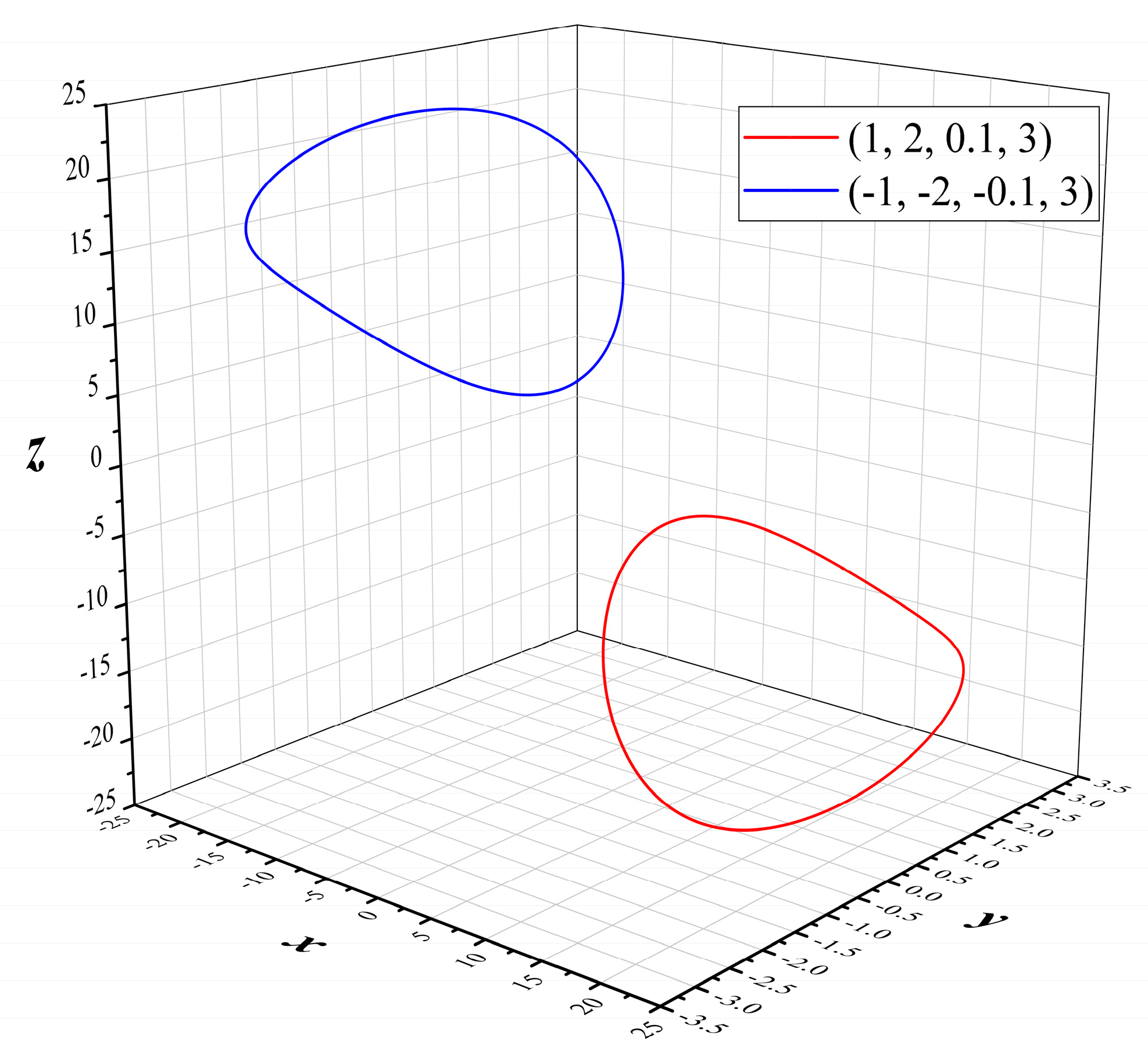
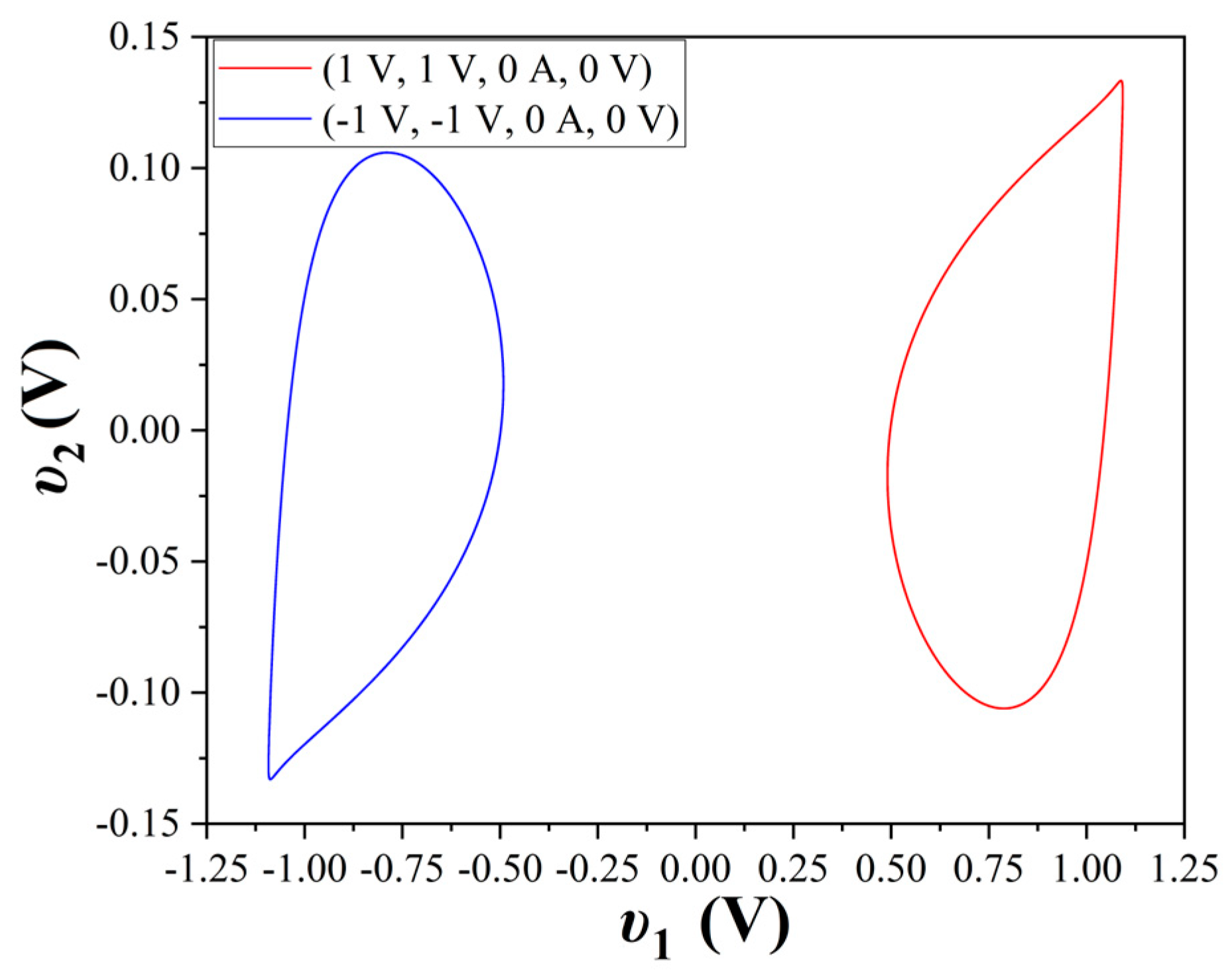
Additionally, the system remains unchanged under the transformation of the coordinates from (x, y, z, w) to (−x, −y, −z, w). Consequently, if (x, y, z, w) constitutes a solution of system (8), then (−x, −y, −z, w) is also a solution. Such symmetry provides an explanation for the occurrence of coexisting attractors in the state space. In Figure 6, the 3D symmetric periodic attractors produced by the numerical simulations of system (8), under the aforementioned transformation, are displayed. Also, the respective symmetric periodic attractors produced by Multisim’s circuit simulation, by changing the initial voltage values of capacitors C₁ and C₂, are depicted in Figure 7.

4. Simulation Results

This section presents the simulation results from both the numerical integration of system (8), using the fourth-order Runge-Kutta algorithm, and also from the simulation of the proposed memristive Chua’s oscillator circuit with Multisim. Moreover, three cases for examining the circuit’s dynamics are outlined. Specifically, by maintaining a constant value for either the element R or C₂, while the value of the other (C₂ or R) varies, intriguing phenomena associated with the circuit’s dynamics are observed. Also, the circuit’s dynamical behavior in regard to the value of the capacitance C is examined in the third case.

4.1. First Case of the Study

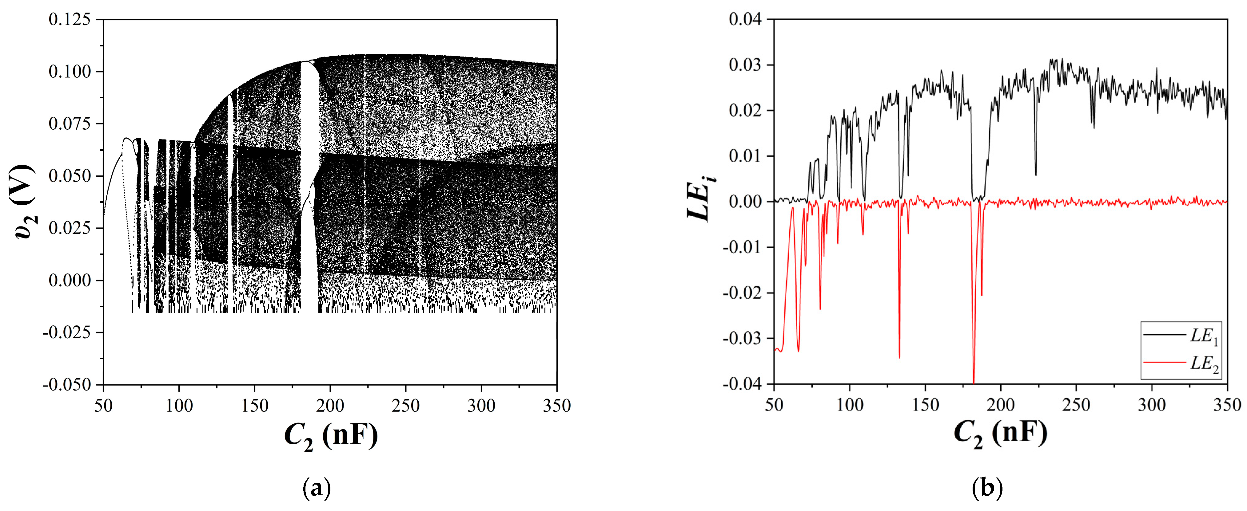
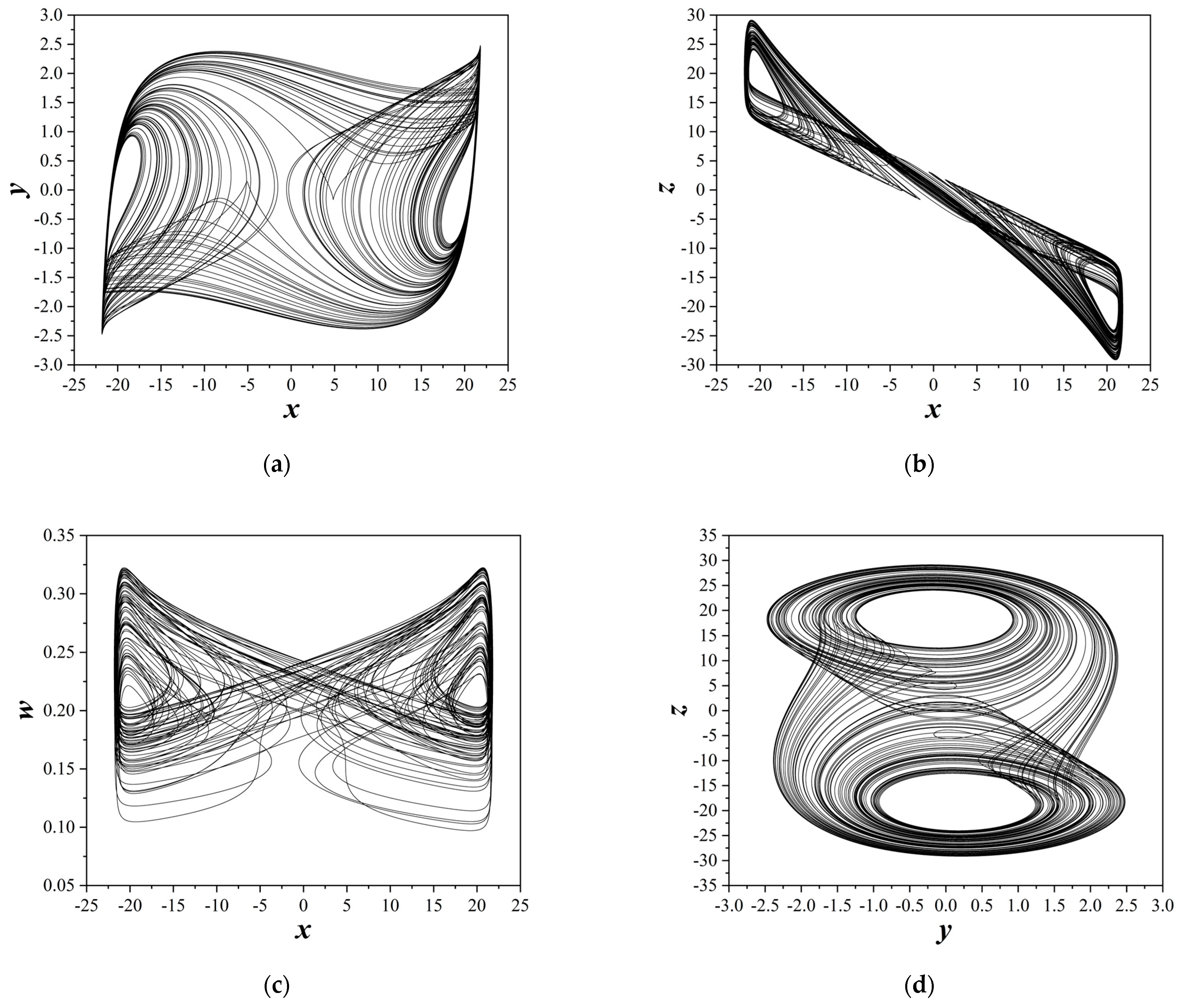
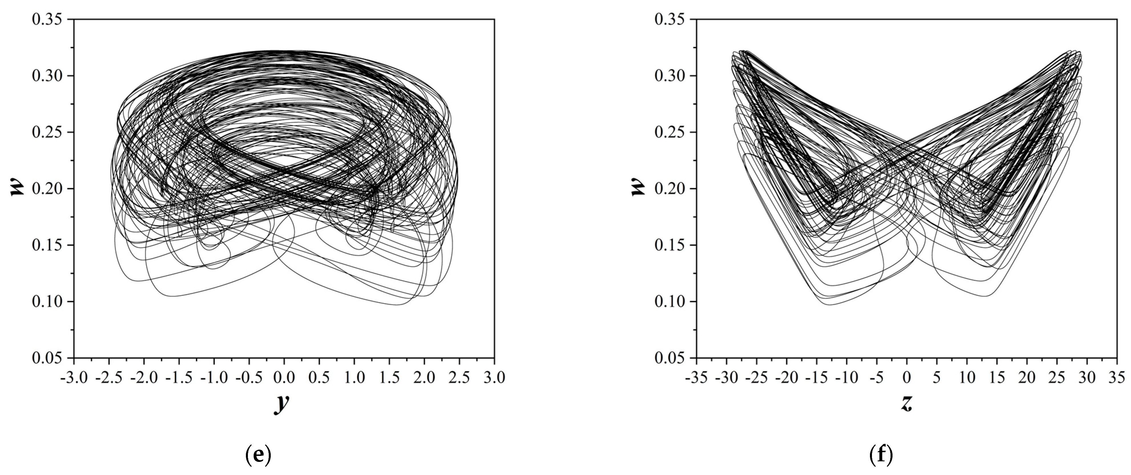
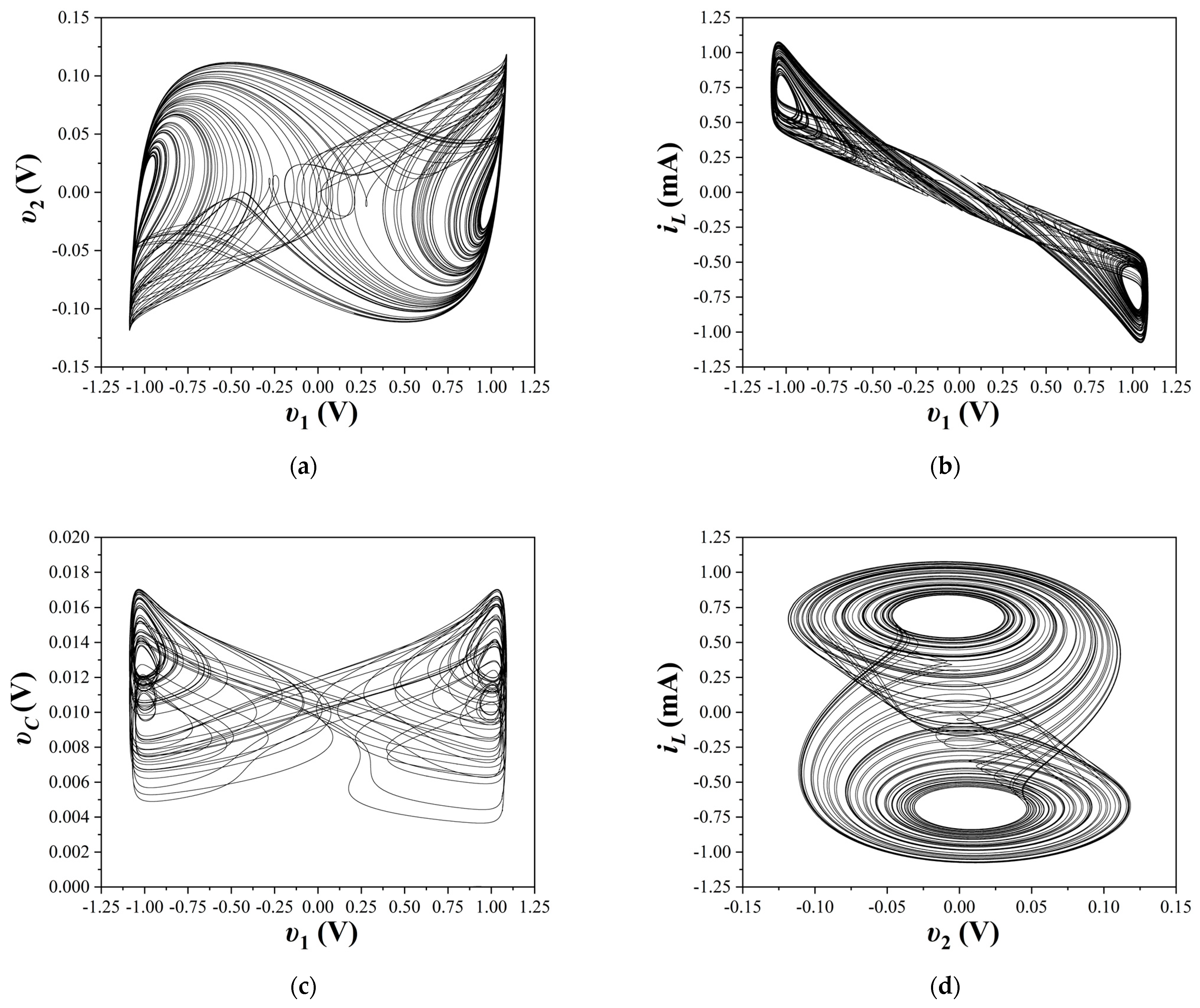
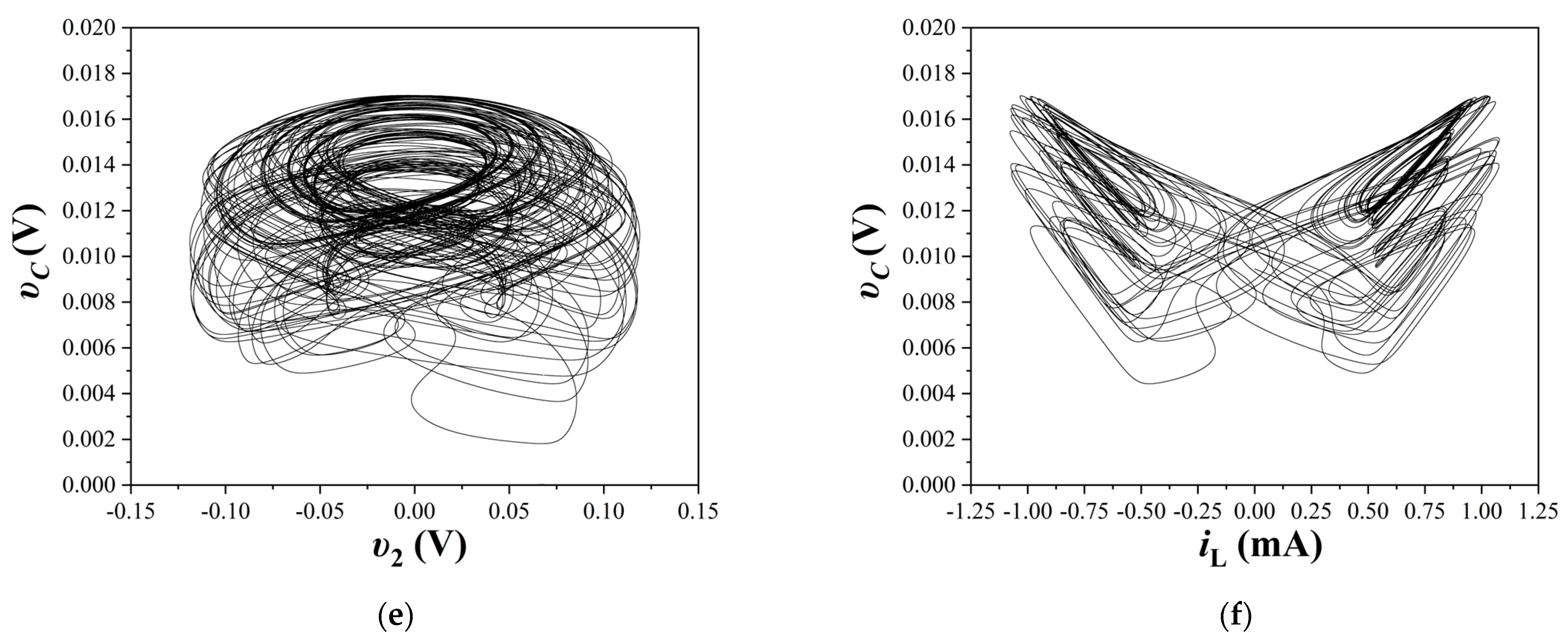
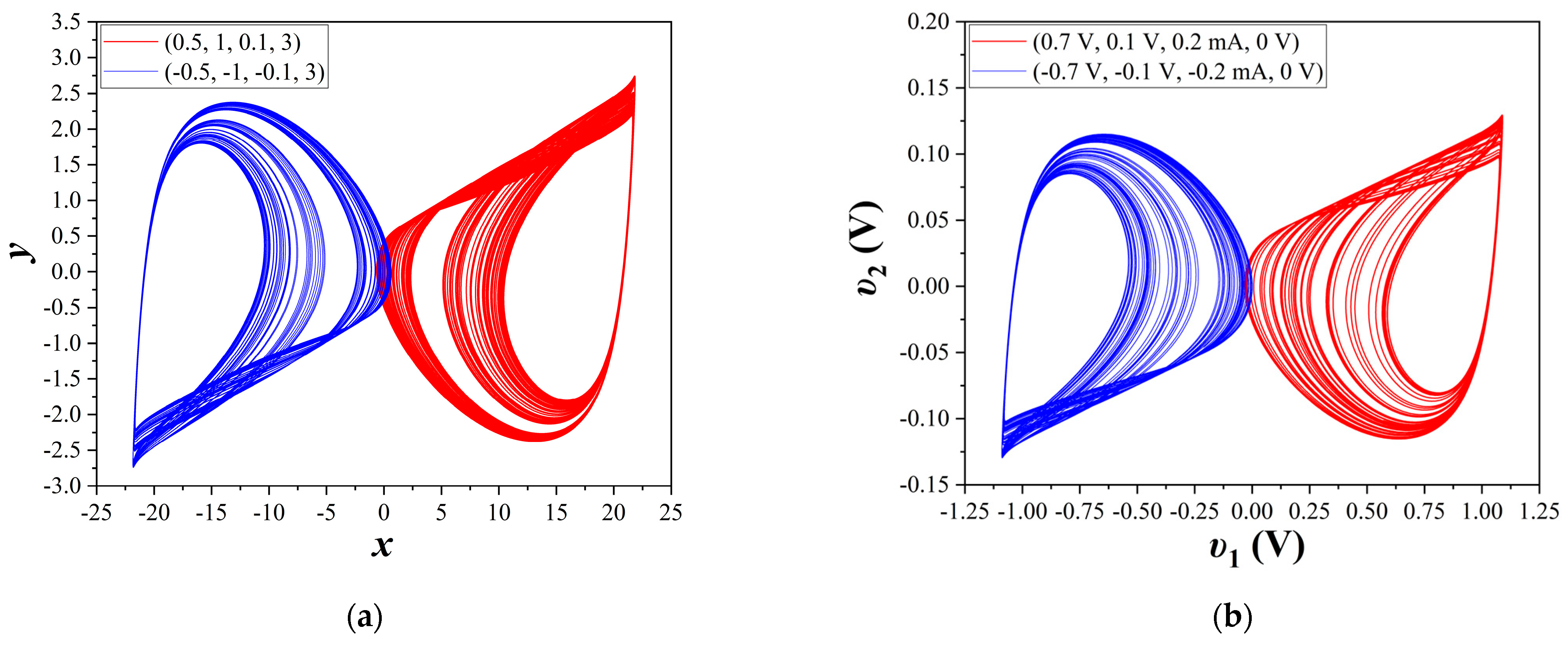
In this case, the value of the resistor R is kept constant (R = 1450 Ω), while the value of the capacitance C₂ serves as the control parameter. The rest of the circuit’s parameters have been chosen as depicted in Table 1 and Table 2. Starting with low values of C₂ = 50 nF, the emergence of two symmetric limit cycles of period-1, as depicted in Figure 6, is observed. With a further increase in the value of C₂, a period-doubling sequences leading to chaos becomes evident. This phenomenon is displayed clearly in the bifurcation diagram of variable y versus the value of the capacitance C₂ (Figure 8a). Also, in Figure 8b, the respective diagram of the two largest Lyapunov exponents of system (8) is depicted, while the other two Lyapunov exponents are omitted because they have both negative values. From this diagram, which is produced by applying Wolf’s algorithm [56], the dynamical behavior of the proposed system is confirmed. As the system is in chaotic regions, it has the largest Lyapunov exponent with a positive value, while it is zero when it is in the periodic regions, which is also observed inside the enlarged chaotic region of the bifurcation diagram of Figure 8a. In Figure 9, the system’s double-scroll chaotic attractors, for C₂ = 170 nF, in various planes are presented. Furthermore, the respective circuit’s chaotic attractors produced from the data, which are captured from Multisim, are depicted in Figure 10. Finally, in Figure 11 two symmetric coexisting chaotic attractors, i.e., for C₂ = 75 nF, which are produced from both the numerical simulation of system (8) and from Multisim, are presented.

4.2. Second Case of the Study

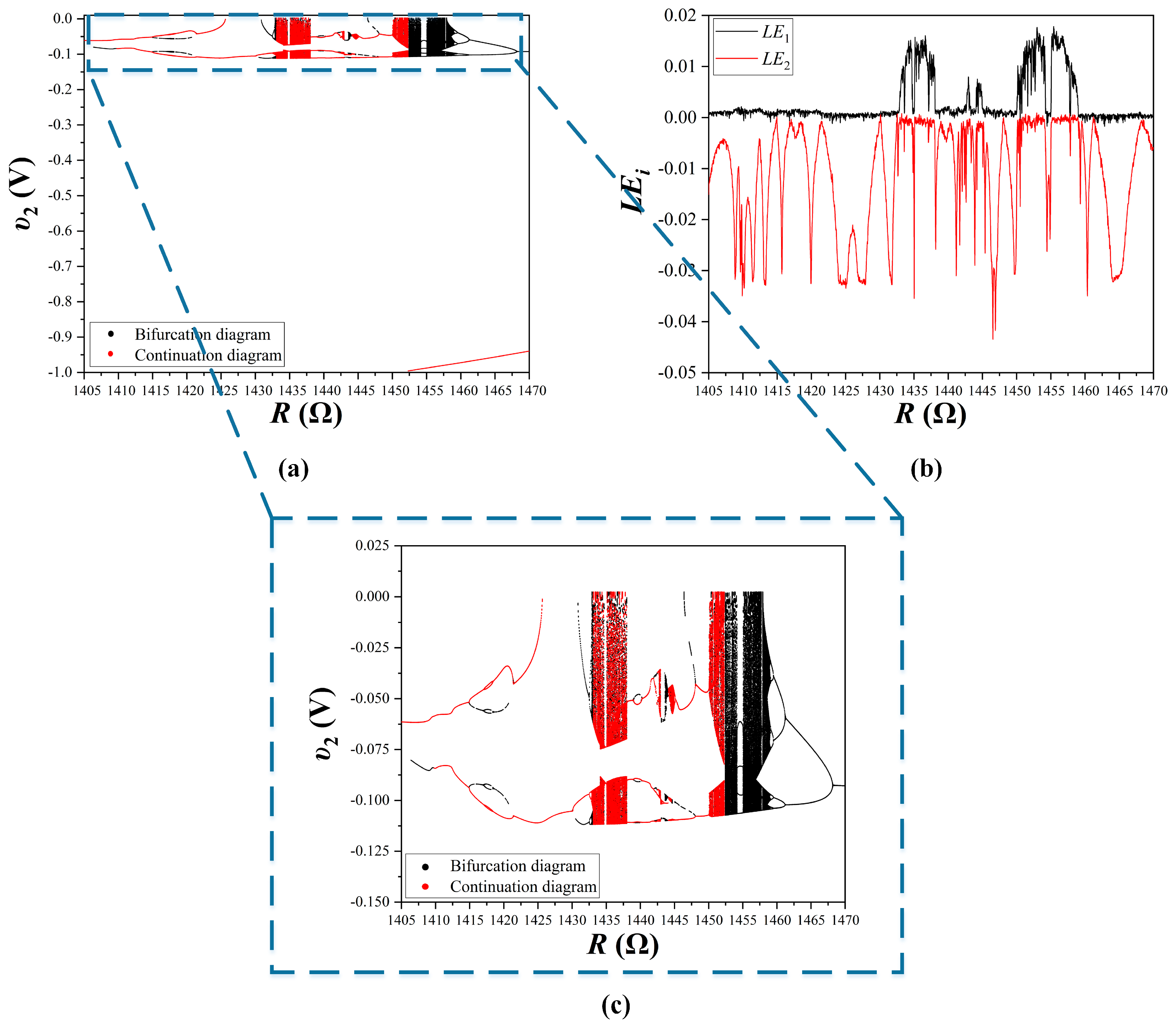
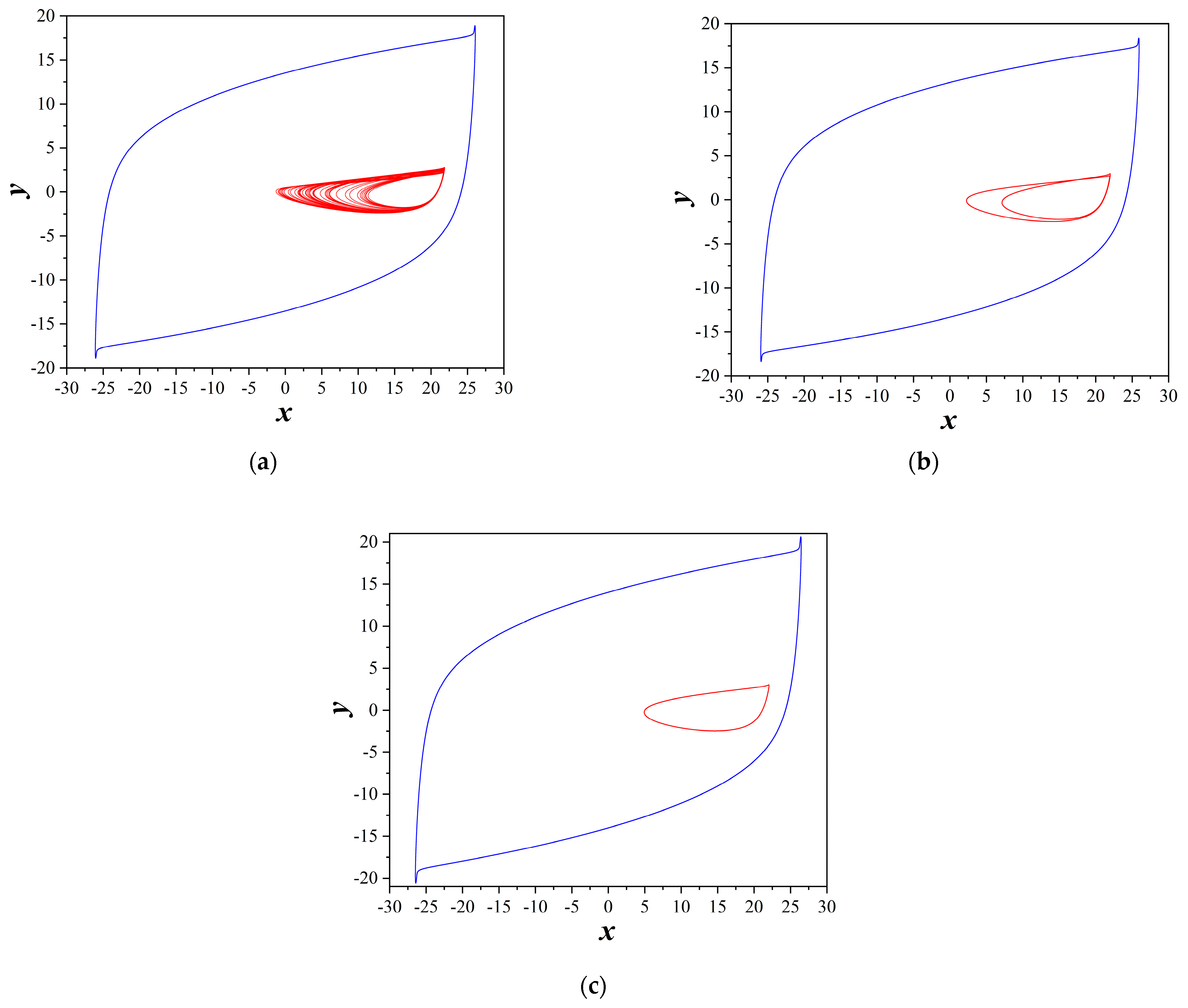
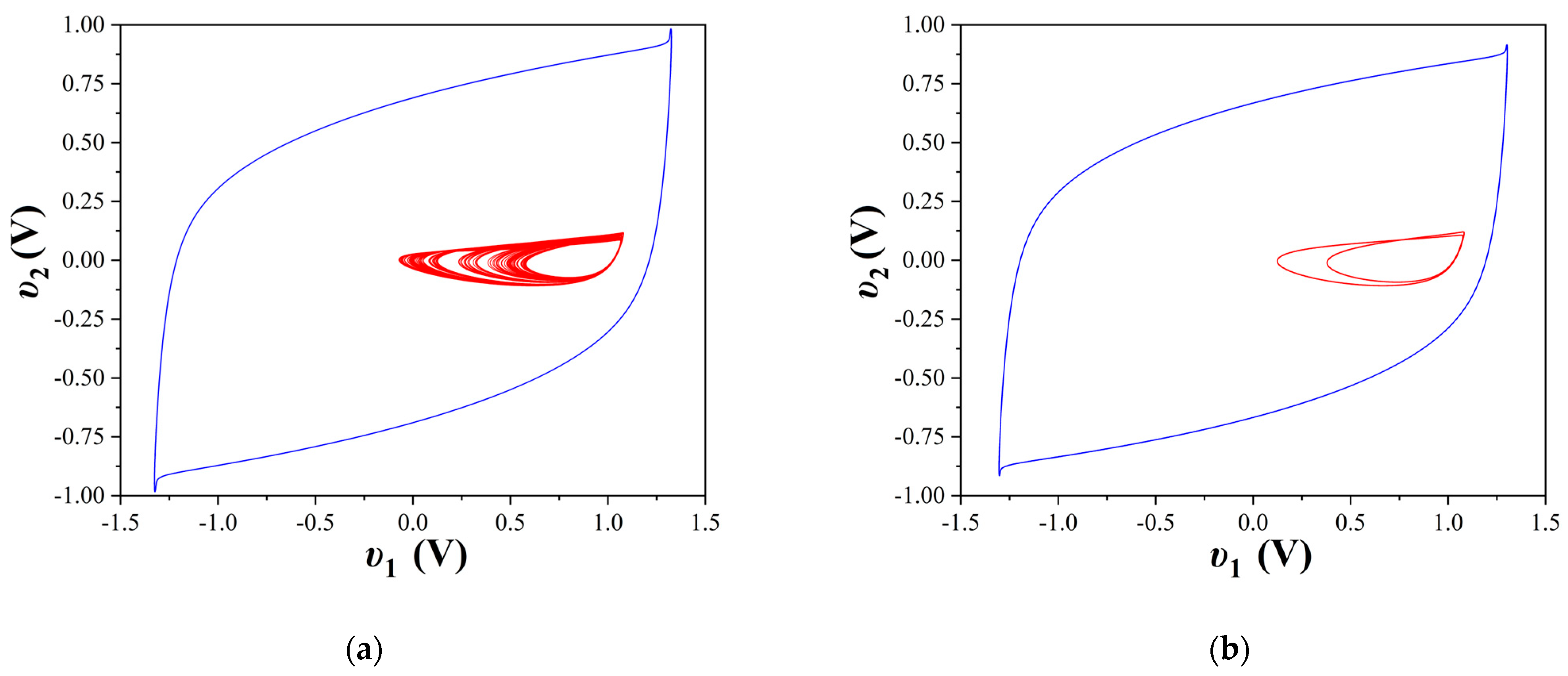
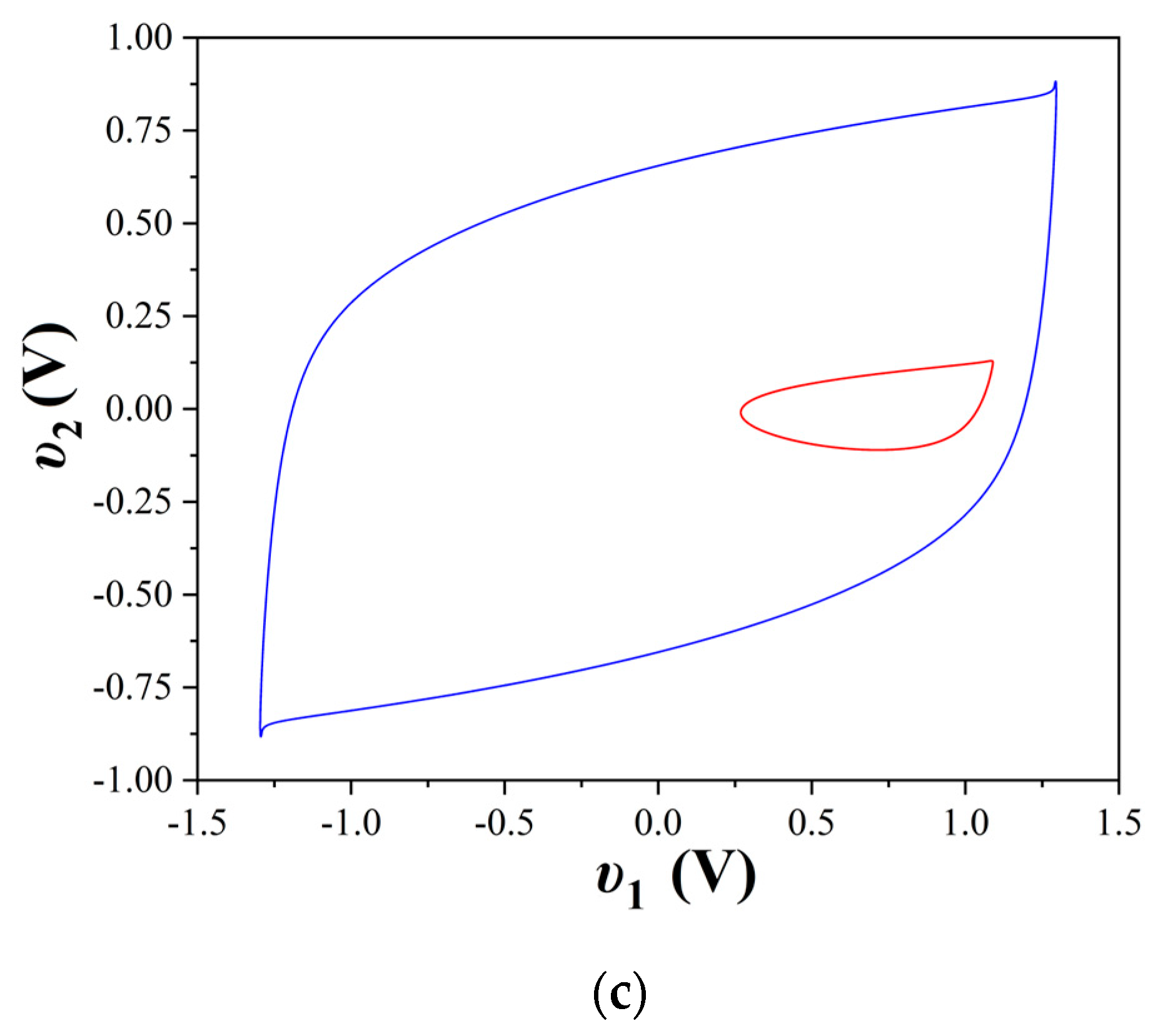
In this case, the capacitance C₂ is held constant (C₂ = 80 nF), while the resistance R plays the role of the control parameter. Also, to reveal the phenomenon of coexisting attractors, the continuation diagram has also been used. Figure 12 displays the continuation diagram concerning the resistance R. The continuation diagram, which is highlighted in red, differs from the corresponding bifurcation diagram, shown in black, based on the choice of initial conditions. Unlike the bifurcation diagram, where the initial conditions remain the same in each iteration, the continuation diagram utilizes the last values of the variables in each iteration as the initial conditions for the subsequent iteration. From the comparison of these two diagrams, coexisting attractors for various values of resistance R are revealed. Figure 13 illustrates three distinct pairs of attractors, for different initial conditions, corresponding to various values of the resistance R, affirming the presence of coexisting attractors. Furthermore, the respective pairs of coexisting attractors produced from Multisim are displayed in Figure 14. In Figure 12b, the spectrum diagram of the Lyapunov exponents (LE) is presented, confirming the chaotic nature of the system through the positive values of the largest Lyapunov exponent.

Moreover, by analyzing the bifurcation diagram of Figure 12, we can observe the occurrence of antimonotonicity. This phenomenon, which was introduced by Dawson et al. [57], is a phenomenon where the system is driven to chaotic behavior as the bifurcation parameter increases. This transition initiates from a period-1 state, following a period-doubling route toward chaos. Subsequently, it exits from the chaotic region, reverting to period-1, through a reverse period-doubling sequence. Furthermore, primary bubbles of period-1 have also been revealed from the bifurcation and continuation diagrams of Figure 12c.

4.3. Third Case of the Study

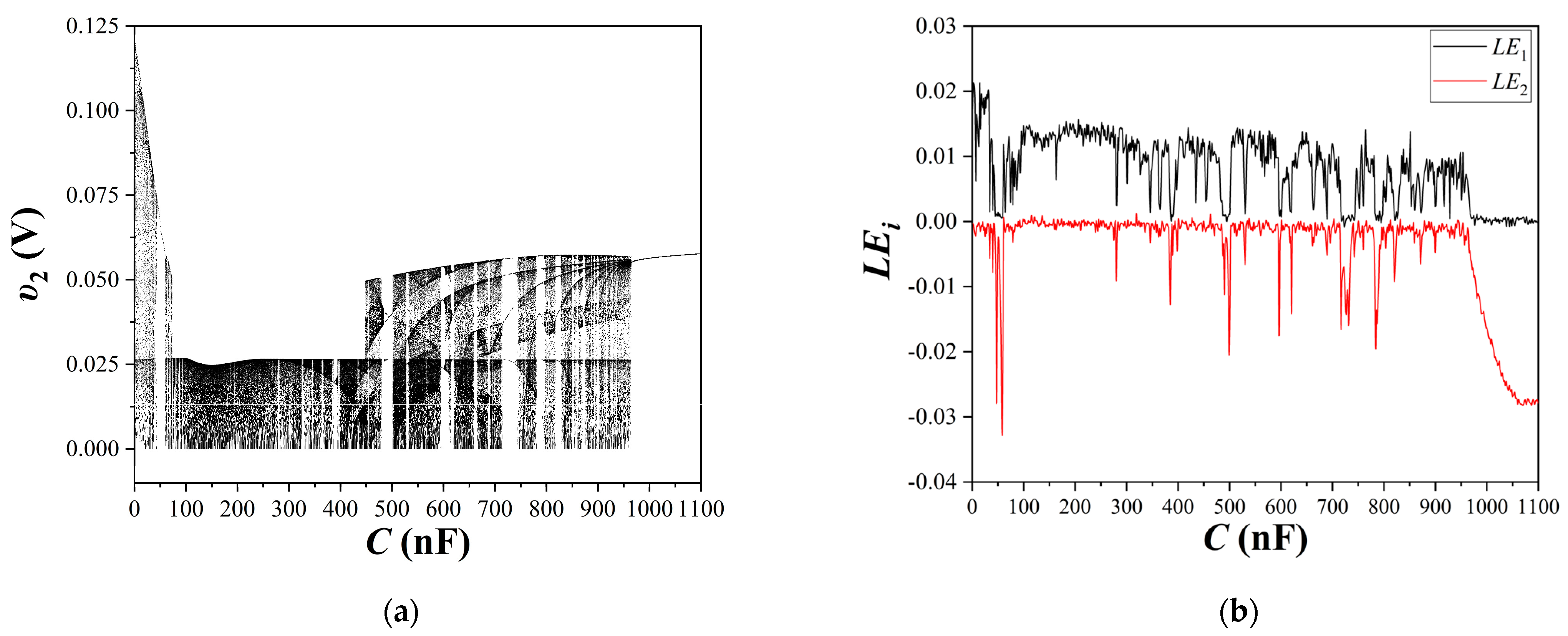
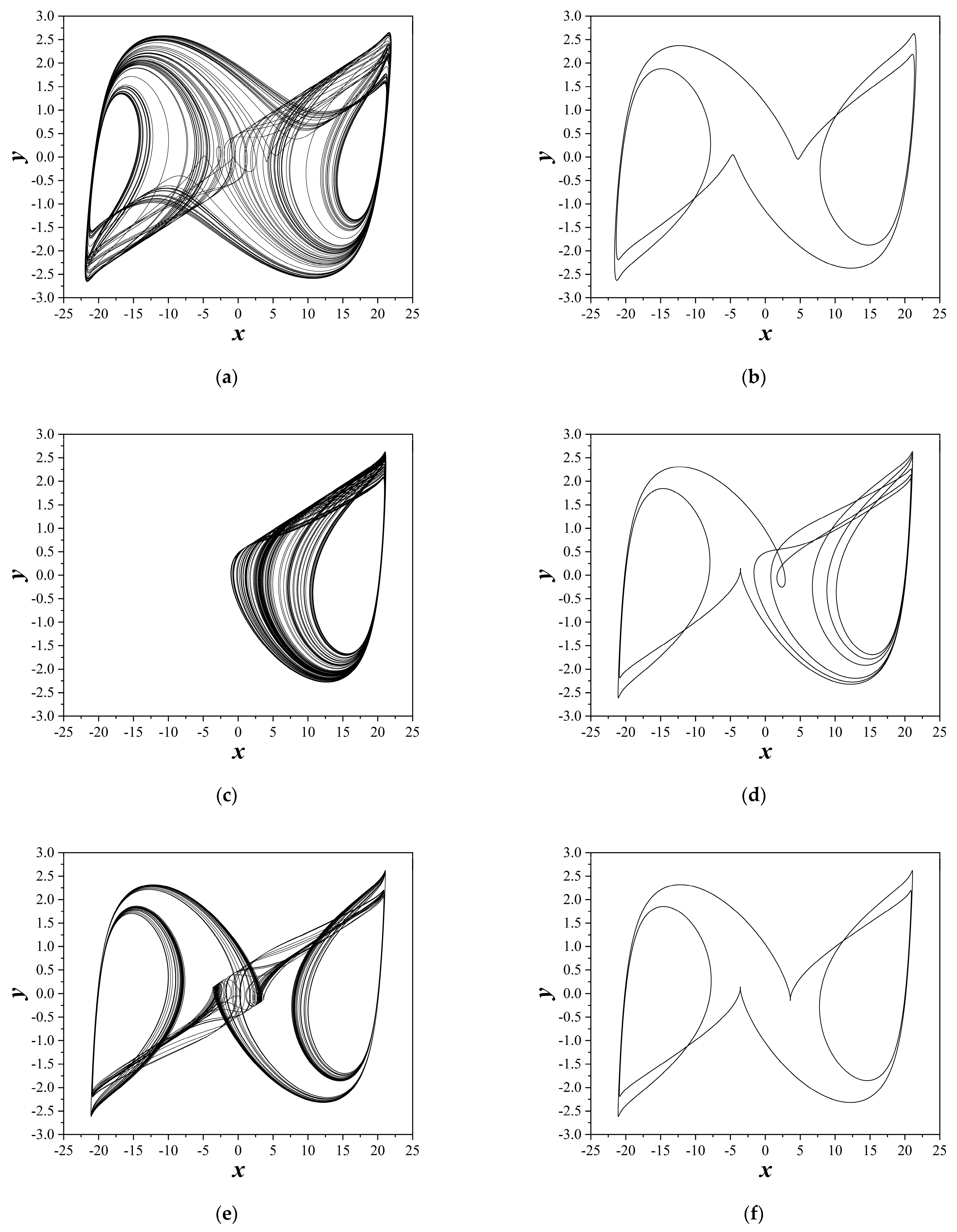
In the third case, the effect of the capacitance C of the memristor’s emulator is studied. For this reason, the rest of the circuit’s parameters have been chosen as depicted in Table 1 and Table 2, while R = 1450 Ω and C₂ = 80 nF. Figure 15a shows the bifurcation diagram of the variable y with respect to the value of capacitance C. This diagram reveals an intricate fractal-like behavior, in its transitions to and from chaos. As the value of the capacitance C increases, the system falls finally into a period-1 behavior, for C ≥ 965.15 nF. As in the previous cases, Figure 15b depicts the diagram of the two largest Lyapunov exponents with respect to the value of the capacitance C, which confirms the circuit’s dynamical behavior, as it is observed from the respective bifurcation diagram. Furthermore, in Figure 16, the circuit’s attractors (periodic and chaotic), in the x–y plane, as they are produced by numerically solving system (8), for various values of the capacitance C, are presented.

5. Conclusions

In this work, a memristive circuit, which is based on Chua’s oscillator, was studied. The specific circuit was designed by using, instead of Chua’s diode, a linear negative resistor, which is coupled with a first-order memristive diode bridge. The study, which was completed, included the analysis of the equilibrium points and their stabilities, as well as the examination of the dynamical characteristics under variations in the circuit parameters through the system’s numerical integration and Multisim simulations. Furthermore, the theoretical analysis revealed that the circuit exhibits two stable conjugate saddle-foci and an unstable saddle equilibrium point. Additionally, the memristive Chua’s oscillator circuit demonstrated diverse dynamical behavior, as evidenced by both the system’s numerical integration and the Multisim simulations. Intriguing phenomena were revealed, including a route to chaos through the period-doubling sequence, coexisting attractors, and the phenomenon of antimonotonicity. An extensive study of the phenomenon of the system’s coexisting attractors, as well as the implementation of the proposed memristive circuit, has been planned for future research, in order to examine its feasibility, as well as its use in a real-world application, such as in a secure communication scheme.

References

- Poincaré, J.H. Sur le problème des trois corps et les équations de la dynamique. Acta Math. 1890, 13, A3–A270. [Google Scholar]
- Lorenz, E.N. Deterministic non-periodic flow. J. Atmos. Sci. 1963, 20, 130–141. [Google Scholar] [CrossRef]
- Mandelbrot, B. The Fractal Geometry of Nature; W.H. Freeman Company: New York, NY, USA, 1977. [Google Scholar]
- Field, R.J.; Györgyi, L. Chaos in Chemistry and Biochemistry; World Scientific Publishing: Singapore, 1993. [Google Scholar]
- Grebogi, C.; Yorke, J. The Impact of Chaos on Science and Society; United Nations University Press: Tokyo, Japan, 1997. [Google Scholar]
- Kyrtsou, C.; Vorlow, C. Complex dynamics in macroeconomics: A novel approach. In New Trends in Macroeconomics; Diebolt, C., Kyrtsou, C., Eds.; Springer: Berlin, Germany, 2005; pp. 223–245. [Google Scholar]
- May, R.M. Theoretical Ecology: Principles and Applications; W.B. Saunders Company: Philadelphia, PA, USA, 1976. [Google Scholar]
- Moon, F.C. Chaotic Vibrations: An Introduction for Applied Scientists and Engineers; Wiley: New York, NY, USA, 1987. [Google Scholar]
- Hasselblatt, B.; Katok, A. A First Course in Dynamics: With a Panorama of Recent Developments; Cambridge University Press: Cambridge, UK, 2003. [Google Scholar]
- Chua, L.O. Chua’s circuit 10 year later. Int. J. Bifurcat. Chaos 1994, 22, 279–305. [Google Scholar] [CrossRef]
- Chua, L.O.; Wu, C.W.; Huang, A.; Zhong, G.Q. A universal circuit for studying and generating chaos—Part I: Routes to chaos. IEEE Trans. Circuits Syst. I 1993, 40, 732–744. [Google Scholar] [CrossRef]
- Chua, L.O.; Wu, C.W.; Huang, A.; Zhong, G.Q. A universal circuit for studying and generating chaos—Part II: Strange attractors. IEEE Trans. Circuits Syst. I 1993, 40, 745–761. [Google Scholar] [CrossRef]
- Fortuna, L.; Frasca, M.; Xibilia, M.G. Chua’s Circuit Implementations: Yesterday, Today and Tomorrow; World Scientific: Singapore, 2009. [Google Scholar]
- Hull, A.W. The dynatron: A vacuum tube possessing negative electric resistance. Proc. Inst. Radio. Eng. 1918, 6, 5–35. [Google Scholar] [CrossRef]
- Brunetti, C. The transitron oscillator. Proc. IRE 1939, 27, 88–94. [Google Scholar] [CrossRef]
- Turner, L.B. The Kallirotron. An aperiodic negative-resitance triode combination. Radio. Rev. 1920, 1, 317–329. [Google Scholar]
- Arns, R.G. The other transistor: Early history of the metal-oxide semiconductor field-effect transistor. Eng. Sci. Educ. J. 1998, 7, 233–240. [Google Scholar] [CrossRef]
- Esaki, L. New phenomenon in narrow germanium p-n junctions. Phys. Rev. 1958, 109, 603. [Google Scholar] [CrossRef]
- Voelcker, J. The Gunn effect. IEEE Spectr. 1989, 26, 24. [Google Scholar] [CrossRef]
- Kennedy, M.P. Robust op amp realization of Chua’s circuit. Frequenz 1992, 46, 66–80. [Google Scholar] [CrossRef]
- Zhong, G.Q.; Ayron, F. Experimental confirmation of chaos from Chua’s circuit. Int. J. Circuit Theory Appl. 1985, 13, 93–98. [Google Scholar] [CrossRef]
- Matsumoto, T. A chaotic attractor from Chua’s circuit. IEEE Trans. Circuits Syst. 1984, 31, 1055–1058. [Google Scholar] [CrossRef]
- Matsumoto, T.; Chua, L.O.; Tokumasu, K. Double scroll via a two-transistor circuit. IEEE Trans. Circuits Syst. 1986, 33, 828–835. [Google Scholar] [CrossRef]
- Cruz, J.M.; Chua, L.O. A CMOS IC Nonlinear Resistor for Chua’s Circuit. IEEE Trans. Circuits Syst. I 1992, 39, 985–995. [Google Scholar] [CrossRef]
- Strukov, D.B.; Snider, G.S.; Stewart, D.R.; Williams, R.S. The missing memristor Found. Nature 2008, 453, 80. [Google Scholar] [CrossRef]
- Chua, L.O. Memristor-The missing circuit element. IEEE Trans. Circuits Syst. I 1971, 18, 507. [Google Scholar] [CrossRef]
- Driscoll, T.; Quinn, J.; Klein, S.; Kim, H.T.; Kim, B.J.; Pershin, Y.V.; Di Ventra, M.; Basov, D.N. Memristive adaptive filters. Appl. Phys. Lett. 2010, 97, 093502. [Google Scholar] [CrossRef]
- Yang, J.J.; Strukov, D.B.; Stewart, D.R. Memristive devices for computing. Nat. Nanotechnol. 2013, 8, 13. [Google Scholar] [CrossRef]
- Adhikari, S.P.; Yang, C.; Kim, H.; Chua, L.O. Memristor Bridge Synapse-Based Neural Network and Its Learning. IEEE Trans. Neural Netw. Learn. Syst. 2012, 23, 1426. [Google Scholar] [CrossRef] [PubMed]
- Volos, C.K.; Kyprianidis, I.M.; Stouboulos, I.N. The memristor as an electric synapse—Synchronization phenomena. In Proceedings of the 2011 17th International Conference on Digital Signal Processing (DSP), Corfu, Greece, 6–8 July 2011; pp. 1–6. [Google Scholar]
- Pershin, Y.V.; Di Ventra, M. Experimental demonstration of associative memory with memristive neural networks. Neural Netw. 2010, 23, 881. [Google Scholar] [CrossRef] [PubMed]
- Wang, L.; Zhang, C.; Chen, L.; Lai, J.; Tong, J. A novel memristor-based rSRAM structure for multiple-bit upsets immunity. IEICE Electron. Expr. 2012, 9, 861. [Google Scholar] [CrossRef]
- Shang, Y.; Fei, W.; Yu, H. Analysis and modeling of internal state variables for dynamic effects of nonvolatile memory devices. IEEE Trans. Circuits Syst. I Regul. Pap. 2012, 59, 1906. [Google Scholar] [CrossRef]
- Shin, S.; Kim, K.; Kang, S.M. Memristor applications for programmable analog ICs. IEEE Trans. Nanotechnol. 2011, 10, 266. [Google Scholar] [CrossRef]
- Itoh, M.; Chua, L.O. Memristor oscillators. Int. J. Bifurcat Chaos 2008, 18, 3183. [Google Scholar] [CrossRef]
- Iu, H.H.C.; Fitch, A.L. Development of Memristor Based Circuits; World Scientific: Singapore, 2013. [Google Scholar]
- Muthuswamy, B. Implementing Memristor based chaotic circuits. Int. J. Bifurcat Chaos 2010, 20, 1335. [Google Scholar] [CrossRef]
- Bao, B.C.; Xu, J.P.; Zhou, G.H.; Ma, Z.H.; Zou, L. Chaotic memristive circuit: Equivalent circuit realization and dynamical Analysis. Chin. Phys. B 2011, 20, 1. [Google Scholar] [CrossRef]
- Li, Y.; Huang, X.; Guo, M. The generation, analysis and circuit implementation of a new memristor based chaotic system. Math. Probl. Eng. 2013, 2013, 398306. [Google Scholar] [CrossRef]
- Buscarino, A.; Fortuna, L.; Frasca, M.; Gambuzza, L.V. A chaotic circuit based on Hewlett-Packard memristor. Chaos 2012, 22, 023136. [Google Scholar] [CrossRef]
- Bao, B.; Yu, J.; Hu, F.; Liu, Z. Generalized memristor consisting of diode bridge with first order parallel RC filter. Int. J. Bifurcat Chaos 2014, 24, 1450143. [Google Scholar] [CrossRef]
- Stork, M. Simple chaotic oscillators with diode bridges. In Proceedings of the 7th IEEE Mediterranean Conference on Embedded Computing (MECO), Budva, Montenegro, 10–14 June 2018; pp. 1–4. [Google Scholar]
- Kengne, J.; Negou, A.N.; Tchiotsop, D. Antimonotonicity, chaos and multiple attractors in a novel autonomous memristor-based jerk circuit. Nonlinear Dyn. 2017, 88, 2589–2608. [Google Scholar] [CrossRef]
- Njitacke, Z.T.; Fotsin, H.B.; Negou, A.N.; Tchiotsop, D. Coexistence of multiple attractors and crisis route to chaos in a novel memristive diode bidge-based Jerk circuit. Chaos Solit Fractals 2016, 91, 180–197. [Google Scholar] [CrossRef]
- Fonzin, T.F.; Srinivasan, K.; Kengne, J.; Pelap, F.B. Coexisting bifurcations in a memristive hyperchaotic oscillator. AEU-Int. J. Electron. Commun. 2018, 90, 110–122. [Google Scholar] [CrossRef]
- Kengne, L.K.; Pone, J.R.M.; Fotsin, H.B. On the dynamics of chaotic circuits based on memristive diode-bridge with variable symmetry: A case study. Chaos Solit. Fractals 2021, 145, 110795. [Google Scholar] [CrossRef]
- Xu, Q.; Cheng, S.; Ju, Z.; Chen, M.; Wu, H. Asymmetric coexisting bifurcations and multi-stability in an asymmetric memristive diode-bridge-based jerk circuit. Chin. J. Phys. 2021, 70, 69–81. [Google Scholar] [CrossRef]
- Wu, H.; Zhou, J.; Chen, M.; Xu, Q.; Bao, B. DC-offset induced asymmetry in memristive diode-bridge-based Shinriki oscillator. Chaos Solit. Fractals 2022, 154, 111624. [Google Scholar] [CrossRef]
- Ramadoss, J.; Kengne, J.; Telem, A.N.K.; Rajagopal, K. Broken symmetry and dynamics of a memristive diodes bridge-based Shinriki oscillator. Phys. A Stat. Mech. Appl. 2022, 588, 126562. [Google Scholar] [CrossRef]
- Chen, M.; Yu, J.; Yu, Q.; Li, C.; Bao, B. A memristive diode bridge-based canonical Chua’s circuit. Entropy 2014, 16, 6464–6476. [Google Scholar] [CrossRef]
- Basha, T.; Mohamed, I.R.; Chithra, A. Design and Study of Memristor based Non-autonomous Chua’s circuit. In Proceedings of the 4th IEEE International Conference on Devices, Circuits and Systems (ICDCS), Coimbatore, India, 16–17 March 2018; pp. 203–206. [Google Scholar]
- Chen, M.; Li, M.; Yu, Q.; Bao, B.; Xu, Q.; Wang, J. Dynamics of self-excited attractors and hidden attractors in generalized memristor-based Chua’s circuit. Nonlinear Dyn. 2015, 81, 215–226. [Google Scholar] [CrossRef]
- Xu, Q.; Wang, N.; Bao, B.; Chen, M.; Li, C. A feasible memristive Chua’s circuit via bridging a generalized memristor. J. Appl. Anal. Comput. 2016, 6, 1152–1163. [Google Scholar]
- Chua, L. Everything you wish to know about memristors but are afraid to ask. In Handbook of Memristor Networks; Springer: Berlin, Germany, 2019; pp. 89–157. [Google Scholar]
- Sprott, J.C.; Wang, X.; Chen, G.R. Coexistence of point, periodic and strange attractors. Int. J. Bifurcat Chaos 2013, 23, 1350093. [Google Scholar] [CrossRef]
- Wolf, A.; Swift, J.B.; Swinney, H.L.; Vastano, J.A. Determining Lyapunov exponents from a time series. Phys. D Nonlinear Phenom. 1985, 16, 285–317. [Google Scholar] [CrossRef]
- Dawson, S.P.; Grebogi, C.; Yorke, J.A.; Kan, I.; Koçak, H. Antimonotonicity: Inevitable reversals of period-doubling cascades. Phys. Lett. A 1992, 162, 249–254. [Google Scholar] [CrossRef]
Figure 1.
The memristor’s emulator. (a) The schematic and (b) the graphical symbol of the memristor.
Figure 2.
Multisim-simulated pinched hysteresis loops of the memristor’s emulator driven by different sinusoidal voltage stimuli , by using (a) = 2 V, with different frequencies and (b) = 1000 Hz, with different voltage amplitudes