A Unified Switched Nonlinear Dynamic Model of an Electric Vehicle for Performance Evaluation

Abstract

The advanced modeling and estimation of overall system dynamics play a vital role in electric vehicles (EVs), as the selection of components in the powertrain and prediction of performance are the key market qualifiers. The state-space averaged model and small-signal transfer function model are useful for assessing long-term behavior in system-level analysis and for designing the controller parameters, respectively. Both models take less computation time but ignore the high-frequency switching dynamics. Therefore, these two models could be impractical for the development and testing of EV prototypes. On the other hand, the multi-domain model in available simulation tools gives in-depth information about the short-term behavior and loss analysis of power electronic devices in each subsystem, considering the switching dynamics in a long computation time. In this paper, a general mathematical framework for the dynamical analysis of complete EVs is presented using a unified, switched nonlinear model. This equation-based model runs faster than the available module-based simulation tools. Two other models, namely the time domain state-space averaged model and frequency domain small-signal transfer function model, are also developed from the switched nonlinear model for the analysis with less computation time. The design and performance of an EV with two different motors and its controllers are evaluated using the general mathematical framework.

1. Introduction

Thriving green energy and a reduction in CO${}_2$ emissions led the transportation industry to develop efficient electrical vehicles (EVs) [1,2]. Development in system simulations plays a vital role in detailed analysis of the system. Vehicle modeling can be in different forms, such as the dynamical model, state-space averaged model, multi-domain simulation model and composite model [3,4]. The reliability and accuracy of the models depend on the consideration of detailed parameters and their interactions. Some imperative effects on vehicle performance, like those from temperature and road conditions, are often neglected for the sake of simplification. As per the intended analysis to be performed on the system, an appropriate simulation method is selected. A multi-domain simulation offers a detailed look into the vehicle dynamics over a steady state simulation, such as load transients and the switching effects of the bidirectional converter and inverter. For example, matlab [5], psim [6], proteus [7] and labview [8] are well equipped with built-in detailed electrical equivalent modules and offer easy-to-use graphical user interfaces at the cost of long simulation times and a lack of insight into the model. Program-based tools such as simplev [9], advisor [10] and v-elph [11] were developed for the selection of components and their efficiency under different operating conditions as well as drive cycles through system-level modeling. To provide quick results [12], these simulation tools use a combination of backward and forward simulation which mostly leans toward backward-facing calculation. But these tools are unable to capture the detailed measurable quantities which are dependent on the component states and computed by integration. For the purpose of powertrain hardware development, forward-facing calculation is preferable to capture the detailed measurable quantities with a small time step.

The main contributions of this paper are the following: (1) a general switched nonlinear model of the EV is developed for performance evaluation while considering the switching effects of the power electronic components, (2) the state-space averaged and small-signal models are derived from the switched nonlinear model to capture the overall slow dynamics and to select and tune the controller parameters, respectively, and (3) therefore, an equation-based unified model is used for design, dynamical analysis, and performance evaluation of EVs.

As this paper is focused on the dynamical modeling, analysis and interaction of the different subsystems in an overall system, the modeling of the thermal management [13], battery management system [14], auxiliary circuit [15] and other protection circuits are not considered. For designing the advanced controller for overall performance optimization of the EV along with efficiency improvement, there are many schemes available in the literature [16,17,18]. In this paper, all these advanced intelligent controllers are also not considered.

The remainder of this paper is organized as follows. Section 2 presents the system’s description and operation. Section 3 deals with the general mathematical framework of EVs and the interaction among different subsystems. The state-space averaged model and small-signal model are presented in Section 4. To validate the models, the performance evaluation of EVs are shown in Section 5. Finally, conclusions are drawn in Section 6.

2. System Description and Operation

A general EV consists of many interconnected subsystems, such as a battery, bidirectional boost–buck converter, three-phase voltage source inverter (VSI), motor and vehicle body, as shown in Figure 1. Depending on the applications and cost requirement, the type of battery (Lead–acid or Li-ion), motor [19,20] (permanent magnet brushless DC motor (BLDC), induction motor (IM), permanent magnet synchronous motor (PMSM) and switched reluctance motor (SRM)) and vehicle body (two-wheeler, three-wheeler, four-wheeler, bus or truck) are selected. In motoring mode, the power is fed to the three-phase inverter-motor combination from the battery through the bidirectional DC-DC converter (boost mode). The bidirectional converter is placed for flexibility of the choice of the rated battery voltage and rated input voltage of the three-phase VSI. The motor is connected to the vehicle body through the transmission system, which consists of fixed gear. During regenerative braking, the power flows in the reverse direction through the VSI and the bidirectional converter (buck mode) to charge the battery. This is a process of recovering the kinetic energy of the motor at the time of braking, which in turn increases the efficiency and range per charge of the overall system [21]. Along with electrical regenerative braking, hydraulic braking is utilized to stop the EV when (1) an emergency stop or a hill climbing or downhill stop is needed or (2) the battery is fully charged or cold.

A two-loop control was selected for the bidirectional boost–buck DC-DC converter. The outer loop and inner loop were implemented to regulate the DC-link voltage (Figure 2) and the battery discharge current through the average current mode control, respectively. To regulate the reference speed, for different motors, different control methods can be used, such as two-loop control (inner current loop and outer speed loop), direct torque control (DTC), field-oriented control (FOC), model predictive control (MPC) or V/f scalar control [22,23,24].

In an EV (Figure 1), the reference speed is given by the drive cycle which, along with the vehicle dynamics, decides the selection of the powertrain parameters. A driving cycle is a series of data points representing the speed of a vehicle versus time. Three different drive cycles were popularly used for the performance evaluation of EVs in different regions in the world [25] namely the New European Driving Cycle (NEDC), United States Federal Test Procedure (US FTP-75) and Japanese Driving Cycle (JC08), but when considering more combinations of vehicle operations and real-world driving behavior, the World Harmonized Light Duty Test Cycle (WLTC) and World Harmonized Light Duty Test Procedure (WLTP) have been established by the United Nations Economic Commission for Europe (UNESE) in a global technical regulation (GTR 15) [26] in 2017. This newly introduced drive cycle also has different classes based on the power-to-mass ratio (PMR) and maximum achievable speed of the selected EV. In this paper, the WLTC Class 1 drive cycle is considered for the test, as given in

Table A1. WLTC Class 1 driving cycle.

Parameter	Value
Distance	8091 m
Total time	1022 s
Idle time	203 s
Maximum speed	64.4 km/h
Maximum acceleration	0.76 m/${\mathrm{s}}^2$
Maximum deceleration	1 m/s${}^2$

.

3. A General Mathematical Framework of an EV Using Switched Nonlinear Modeling

The overall switched nonlinear dynamic model of an EV was implemented step by step by considering the differential equations in each subsystem as well as the interaction among subsystems given in Figure 2.

3.1. Mathematical Model of the Battery

The choice as well as the dynamic model of the battery are very important for the performance and range of the EV. From different battery technologies, such as lead–acid, lithium-ion (Li-ion) nickel–cadmium (Ni-Cd) and nickel–metal hydride (NiMH), Li-ion is predominantly preferred due to its high energy density, low self discharge, long cycle life and high intrinsic safety [27].

For mathematical modeling of the battery, there are different techniques, such as the electrochemical mechanism model, electro-thermal model, equivalent circuit model (ECM) and data-driven models, with their advantages and disadvantages [28,29]. In general, more complex models give accurate results at the cost of higher computational efforts and time-consuming and costly laboratory testing for parameter identification. For example, in the case of the equivalent circuit model, its accuracy can be increased with a high number of parallel RC groups [30], but two RC groups has shown the trade-off between accuracy and complexity [31]. In most of the cases, the parameter values are given for one cell [32]. For modeling a battery pack of a specific rating, the scaling of the cell parameters is carried out based on the series and parallel connections of the battery cells [33].

It is important to note that the modeling of a battery solely depends on the accurate estimation of the state of charge (SoC) of the battery [32]. The SoC also determines the safe charging and discharging, optimal usage of battery and range prediction for an EV. Moreover, the battery model parameters are nonlinear in terms of the SoC, temperature, current rate, aging of the battery, self-discharge, hysteresis, etc. 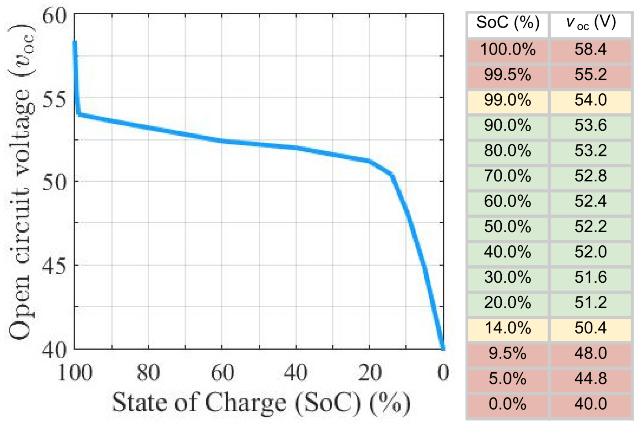To bypass the complicated optimization techniques and sophisticated algorithm for SoC estimation [34], one can use the discharge curve from the manufacturer’s datasheet. A typical discharge curve relates the change in battery capacity (Q) to the open circuit voltage ($v_{\mathrm{oc}}$). Only three points on the manufacturer’s discharge curve in a steady state are required to extract parameters from an equation-based battery discharge/charge model [35]. To further simplify the process, one can construct the SoC versus open-circuit voltage ($v_{\mathrm{oc}}$) curve directly using limited points from the look-up table of the manufacturer’s datasheet, which is the outcome of the experimental data [28].

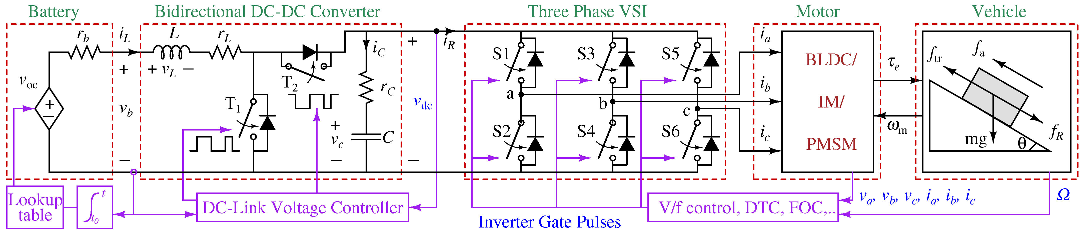
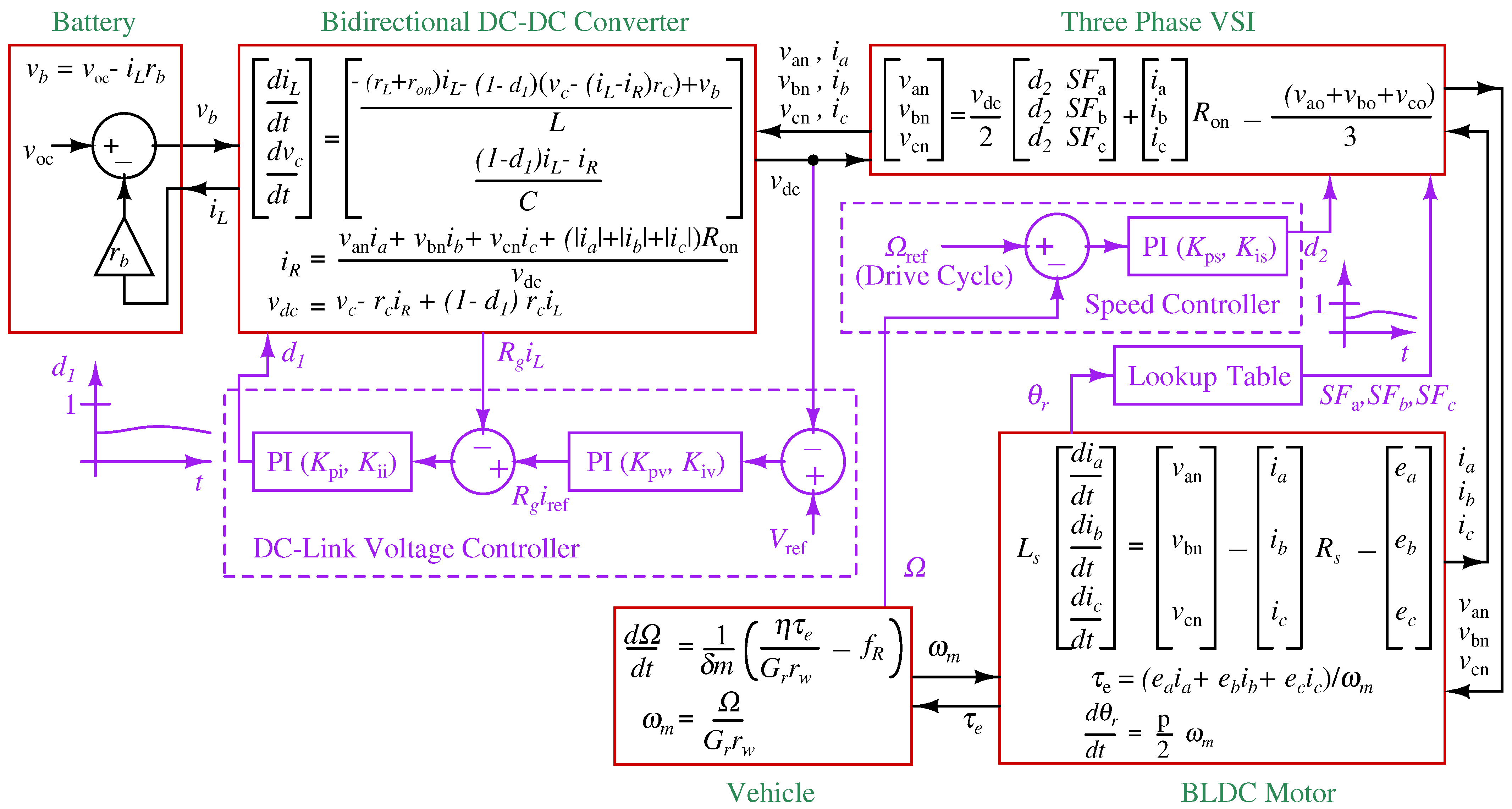
In this paper, the battery model is obtained while considering the SoC-dependent open-circuit voltage with the series internal resistance, as shown in the battery subsystem in Figure 2. The SoC is calculated using the Coulomb counting method by integration of the measured current. Then, the open-circuit voltage is determined from the predefined look-up table. Due to the flat nature of the discharge curve (Figure 3), the two successive points are connected using a straight-line equation.

The equations of the battery are as follows:

$$v_b=v_{\mathrm{oc}}\left(SoC\right)-i_L{r}_b,p_b=i_L^2{r}_b,E_b={\int }_{t_0}^t{p}_{b}d\tau$$

(1)

$$SoC\left(t\right)=SoC\left(t_0\right)-100{\int }_{t_0}^t\frac{i_L\left(\tau \right)}{({\eta }_b\times Q_{\mathrm{bat}}\times 3600)}d\tau$$

(2)

where the battery open circuit voltage ($v_{\mathrm{oc}}$), internal resistance ($r_b$), nominal or rated battery capacity ($Q_{\mathrm{bat}}$), battery efficiency (${\eta }_b$) and initial battery state of charge ($SoC\left(t_0\right)$) are the specified parameters of the battery. As the Coulomb counting method gives the relative change in SoC and not an absolute value, the $SoC\left(t_0\right)$ is calculated by fully charging the battery pack to a known voltage, which is available from the manufacturer’s datasheet. But the current ($i_L$) is calculated from the bidirectional boost–buck DC-DC converter. The battery terminal voltage ($v_b$), power loss ($p_b$), energy transferred ($E_b$) and state of charge of the battery ($SoC$) are calculated over the selected drive cycle to obtain the range of the EV in a single charge.

3.2. Mathematical Model of the Bidirectional DC-DC Converter and DC-Link Voltage Controller

The battery is connected to the DC-link through a bidirectional DC-DC converter. As per the mode of operations, the converter switches (${\mathrm{T}}_1$ and ${\mathrm{T}}_2$ in Figure 2) are turned on alternately to control the current flow bidirectionally by maintaining the DC-link voltage. The inductor current ($i_L$) and capacitor voltage ($v_c$) are calculated as follows [37]:

$$\begin{array}{ccc}\hfill i_L& =& \frac{1}{L}\int \left(v_L-(r_L+r_{\mathrm{on}})i_L\right)dt\hfill \\ \hfill \Rightarrow i_L& =& \frac{1}{L}\int \left(v_{b}F+(v_b-v_{\mathrm{dc}})\overline{F}-(r_L+r_{\mathrm{on}})i_L\right)dt\hfill \end{array}$$

(3)

$$\begin{array}{ccc}\hfill v_c& =& \frac{1}{C}\int i_{C}dt\hfill \\ \hfill \Rightarrow v_c& =& \frac{1}{C}\int (-i_R+i_L\overline{F})dt\hfill \end{array}$$

(4)

$$\begin{array}{ccc}\hfill v_{\mathrm{dc}}& =& v_c-r_c{i}_R+r_c{i}_L\overline{F}\hfill \end{array}$$

(5)

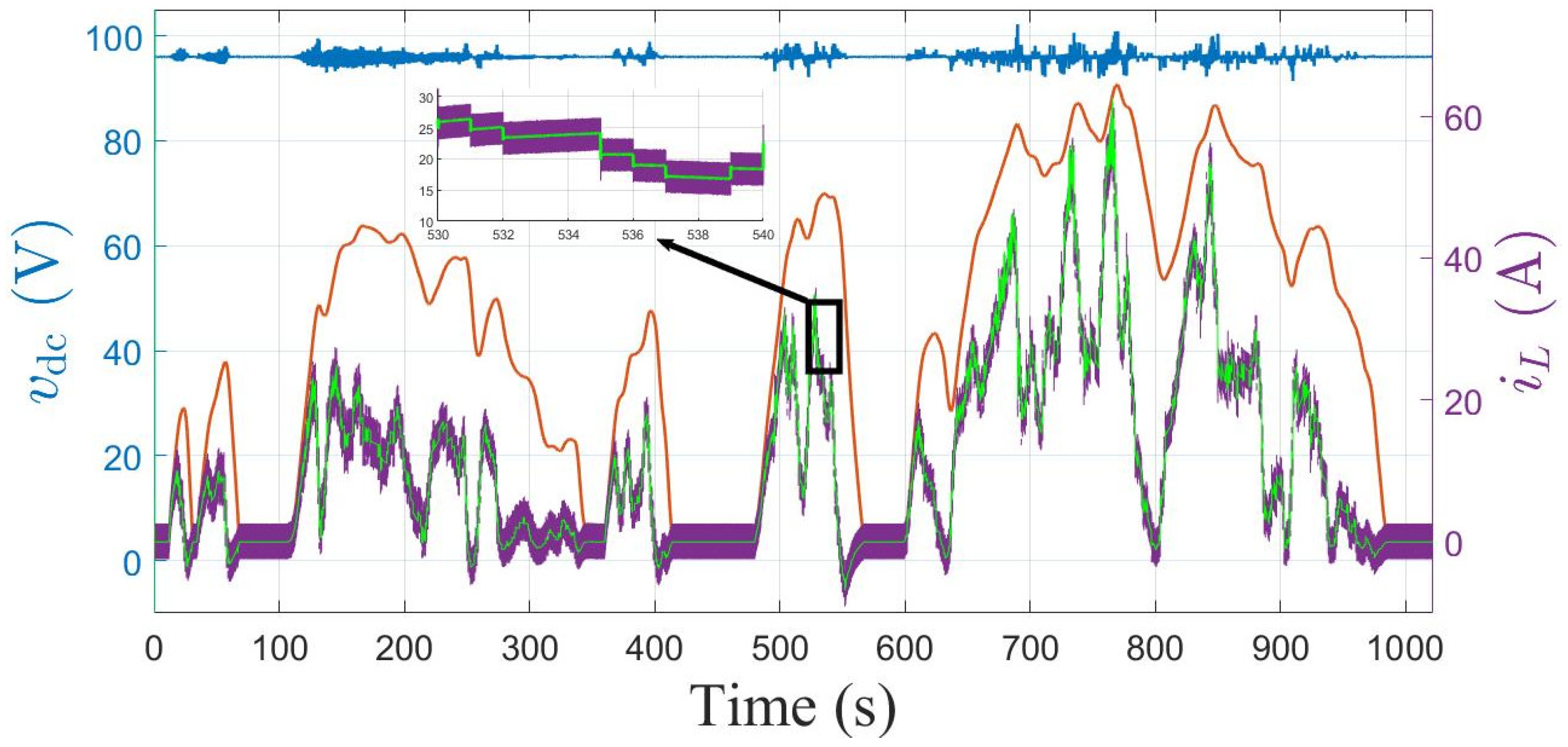
where L, $r_L$, C and $r_C$ are the inductance, series resistance of the inductor, capacitance and its equivalent series resistance (ESR), respectively, F is the switching signal given to $T_1$ based on the feedback control law given in Equation (8), $\overline{F}$ is the complimentary signal for $T_2$ and $i_R$ is the input current of the three-phase VSI. Then, the DC-link voltage ($v_{\mathrm{dc}}$) is calculated, and this is connected to the three-phase VSI (Figure 2). The same equations are solved for motoring (boost mode) as well as regenerative braking (buck mode). The motoring or regenerative braking operation is decided by the sign of $i_R$, which is the load current of the bidirectional DC-DC converter, as shown in Figure 2.

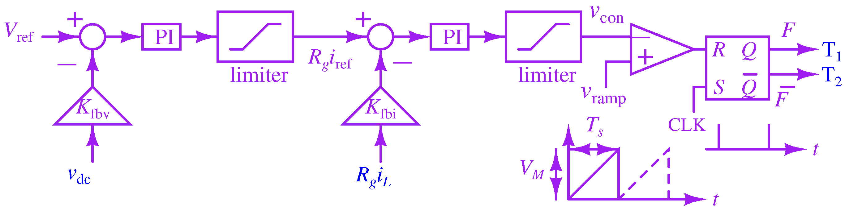
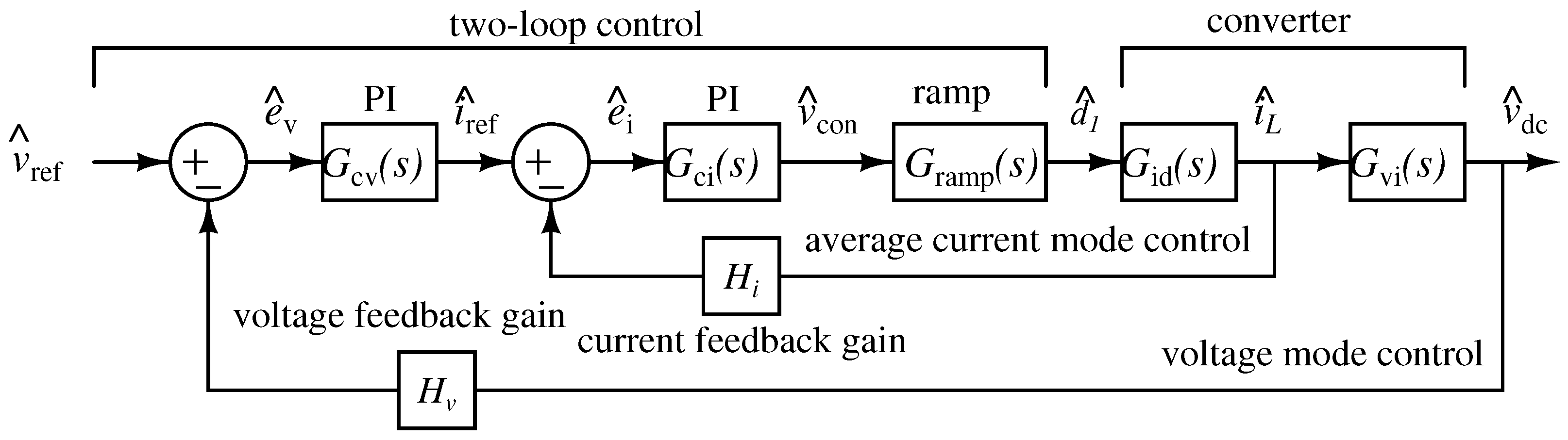
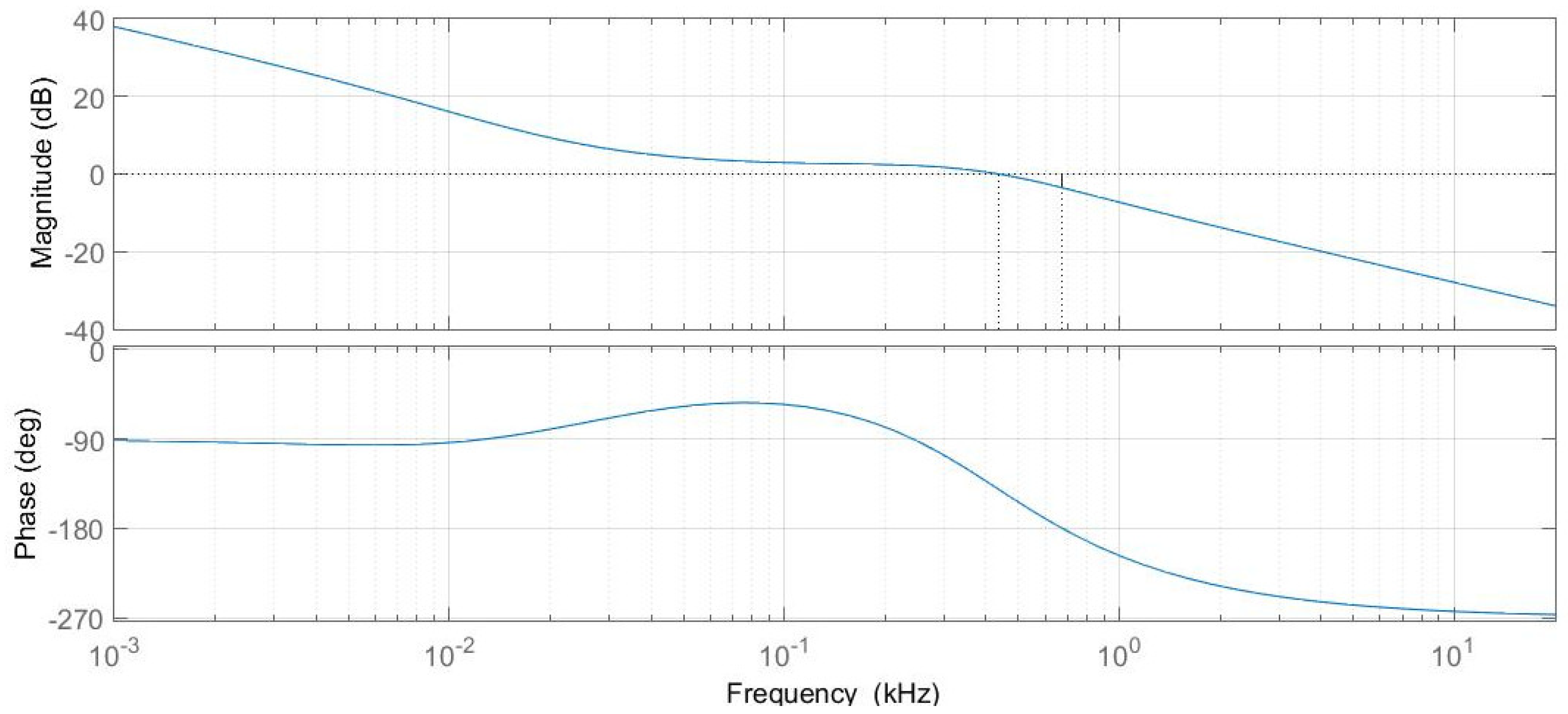
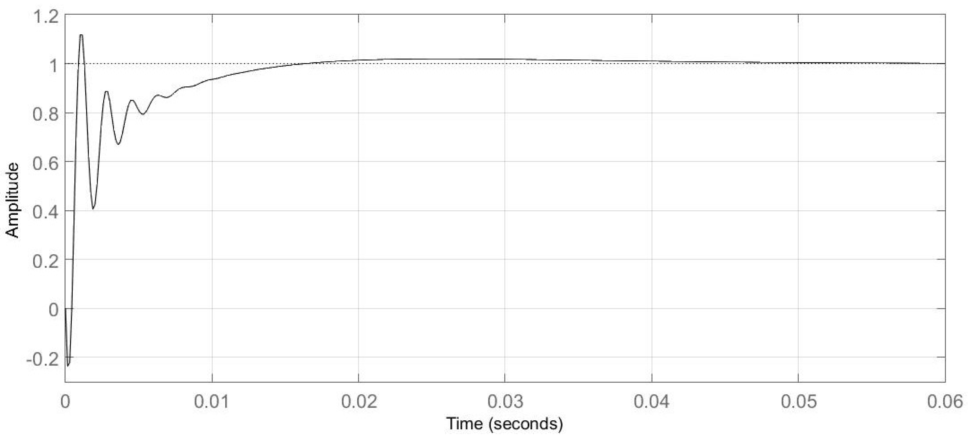
A two-loop control is used to regulate the DC-link voltage as shown in Figure 4. In comparison with the outer voltage loop, the inner current loop has faster dynamics as it considers the faster change in the inductor current dynamics. In the outer voltage control loop, the sensed DC-link voltage is subtracted from the reference voltage ($V_{\mathrm{ref}}$) and passed through a PI compensator to generate the current reference ($R_g{i}_{\mathrm{ref}}$) for the inner loop. Then, the sensed inductor current signal ($R_g{i}_L$) is subtracted from the current reference, where $R_g$ is the sensor gain. The difference is sent through a PI compensator to generate the control voltage ($v_{\mathrm{con}}$). Two PI controllers are designed using a small-signal model, which is given in Section 4. The reference signal and control voltage are as follows:

$$\begin{array}{ccc}\hfill R_g{i}_{\mathrm{ref}}& =& K_{\mathrm{pv}}(V_{\mathrm{ref}}-K_{\mathrm{fbv}}{v}_{\mathrm{dc}})+K_{\mathrm{iv}}\int (V_{\mathrm{ref}}-K_{\mathrm{fbv}}{v}_{\mathrm{dc}})dt\hfill \end{array}$$

(6)

$$\begin{array}{ccc}\hfill v_{\mathrm{con}}& =& K_{\mathrm{pi}}(R_g{i}_{\mathrm{ref}}-K_{\mathrm{fbi}}{R}_g{i}_L)+K_{\mathrm{ii}}\int (R_g{i}_{\mathrm{ref}}-K_{\mathrm{fbi}}{R}_g{i}_L)dt\hfill \end{array}$$

(7)

where $K_{\mathrm{pv}}$, $K_{\mathrm{iv}}$, $K_{\mathrm{pi}}$ and $K_{\mathrm{ii}}$ are the compensator gains and $K_{\mathrm{fbv}}$ and $K_{\mathrm{fbi}}$ are the feedback gains. The switch ${\mathrm{T}}_1$ is periodically turned on at the start of each switching cycle as the clock signal (CLK) is applied to the set pin of the flip-flop. Then, the control voltage is compared with a unipolar sawtooth carrier signal ($v_{\mathrm{ramp}}$) to reset the flip-flop. The flip-flop is used to avoid multiple switching instances within a clock period. In this process, the switching pulses F and $\overline{F}$ are generated for ${\mathrm{T}}_1$ and ${\mathrm{T}}_2$. The control logic is given by

$$\mathrm{if}{v}_{\mathrm{con}}\ge v_{\mathrm{ramp}}\mathrm{then}F=1,\mathrm{otherwise}F=0$$

(8)

where $v_{\mathrm{ramp}}=V_M\left(t\mathrm{mod}{T}_s\right)$, $V_M$ is the amplitude and $T_s$ denotes the switching period.

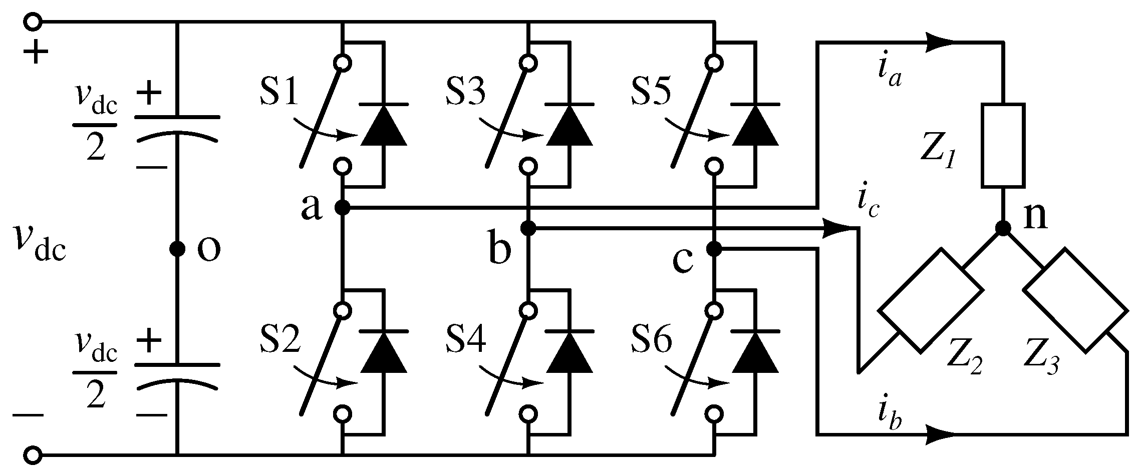
3.3. Mathematical Model of the Three-Phase VSI

By considering the voltage drop across the switch but with zero leakage current and zero for the rise and fall times of the waveforms of the switches, the inverter is simplified. As shown in Figure 5, the relation between the input DC-link voltage ($v_{\mathrm{dc}}$) and output three phase voltages ($v_{\mathrm{an}},v_{\mathrm{bn}},v_{\mathrm{cn}}$) is established using six switching signals. These six signals can simply be used as the three switching functions for three legs of the inverter [38]. The switching functions can be represented in terms of the gate pulses ($u_1$, $u_2$, $u_3$, $u_4$, $u_5$, $u_6$) of six switches ($\mathrm{S}1,\mathrm{S}2,\mathrm{S}3,\mathrm{S}4,\mathrm{S}5,\mathrm{S}6$):

$$S{F}_a=u_1-u_2,S{F}_b=u_3-u_4,S{F}_c=u_5-u_6$$

When the two switches in a leg are off, then the switching functions are zero. In a leg, both switches cannot be turned on simultaneously. Therefore, based on the switching combinations, the switching functions are

$$\begin{array}{c}\hfill S{F}_a=1\left(\mathrm{S}1\mathrm{ON}\mathrm{and}\mathrm{S}2\mathrm{OFF}\right),S{F}_a=-1\left(\mathrm{S}1\mathrm{OFF}\mathrm{and}\mathrm{S}2\mathrm{ON}\right)\\ \hfill S{F}_b=1\left(\mathrm{S}3\mathrm{ON}\mathrm{and}\mathrm{S}4\mathrm{OFF}\right),S{F}_b=-1\left(\mathrm{S}3\mathrm{OFF}\mathrm{and}\mathrm{S}4\mathrm{ON}\right)\\ \hfill S{F}_c=1\left(\mathrm{S}5\mathrm{ON}\mathrm{and}\mathrm{S}6\mathrm{OFF}\right),S{F}_c=-1\left(\mathrm{S}5\mathrm{OFF}\mathrm{and}\mathrm{S}6\mathrm{ON}\right)\end{array}$$

The generated voltage in every phase considering voltage drop due to the resistance when turned on ($R_{\mathrm{on}}$ = 28 m$\mathsf{\Omega }$) for the switch can be written as

$$v_{\mathrm{an}}=v_{\mathrm{ao}}-v_{\mathrm{no}},v_{\mathrm{bn}}=v_{\mathrm{bo}}-v_{\mathrm{no}},v_{\mathrm{cn}}=v_{\mathrm{co}}-v_{\mathrm{no}}$$

(9)

where $v_{\mathrm{ao}}$, $v_{\mathrm{bo}}$, $v_{\mathrm{co}}$ and $v_{\mathrm{no}}$ can be obtained as follows:

$$\left[\begin{array}{c}{v}_{\mathrm{ao}}\\ v_{\mathrm{bo}}\\ v_{\mathrm{co}}\end{array}\right]=\frac{v_{\mathrm{dc}}}{2}\left[\begin{array}{c}S{F}_a\\ S{F}_b\\ S{F}_c\end{array}\right]+\begin{array}{c}\left[\begin{array}{c}{i}_a\\ i_b\\ i_c\end{array}\right]R_{\mathrm{on}}\end{array},\begin{array}{c}{v}_{\mathrm{no}}=\frac{1}{3}(v_{\mathrm{ao}}+v_{\mathrm{bo}}+v_{\mathrm{co}})\end{array}$$

(10)

3.4. Mathematical Model of Motors and Controllers

The most important part of the EV is the motor, which needs to be chosen very carefully by considering the advantages and disadvantages of a specific kind of motor for a particular drive [39,40]. The proposed mathematical framework provides flexibility in the choice of the motor for the vehicle as well as the drive cycle. Two motors are used in this paper with two different kinds of controllers for performance evaluation using the switched nonlinear dynamic model.

3.4.1. BLDC with a Single-Loop Speed Controller

Most electric two- and three-wheelers are using BLDC because of its very low weight, comparative high efficiency and low maintenance [41]. This motor can be modeled using a set of differential equations.

Using Figure 6, the stator currents of the BLDC motor are calculated from the following set of differential equations [42]:

$$\begin{array}{ccc}\hfill \frac{d{i}_a}{dt}& =& \frac{1}{L_s}(v_{\mathrm{an}}-e_a-R_s{i}_a)\hfill \\ \hfill \frac{d{i}_b}{dt}& =& \frac{1}{L_s}(v_{\mathrm{bn}}-e_b-R_s{i}_b)\hfill \\ \hfill \frac{d{i}_c}{dt}& =& \frac{1}{L_s}(v_{\mathrm{cn}}-e_c-R_s{i}_c)\hfill \end{array}$$

(11)

The stator currents of the three phases can also be calculated using the line-line voltages at the input terminal (i.e., the phase voltages of the inverter) along with the stator inductance ($L_s$), stator resistance ($R_s$) and back EMFs:

$$\begin{array}{ccc}\hfill \frac{d{i}_a}{dt}& =& \frac{1}{3L_s}(2v_{\mathrm{ab}}+v_{\mathrm{bc}}-2e_a+e_b+e_c-3R_s{i}_a)\hfill \end{array}$$

(12)

$$\begin{array}{ccc}\hfill \frac{d{i}_b}{dt}& =& \frac{1}{3L_s}(-v_{\mathrm{ab}}+v_{\mathrm{bc}}+e_a-2e_b+e_c-3R_s{i}_b)\hfill \end{array}$$

(13)

$$\begin{array}{ccc}\hfill i_c& =& -i_a-i_b\hfill \end{array}$$

(14)

The back EMFs are calculated as follows:

$$\left[\begin{array}{c}{e}_a\\ e_b\\ e_c\end{array}\right]=\frac{K_E}{2}{\omega }_m\left[\begin{array}{c}cos\left({\theta }_r\right)\\ cos({\theta }_r-\frac{2\pi }{3})\\ cos({\theta }_r+\frac{2\pi }{3})\end{array}\right]$$

(15)

where the back EMF constant is $K_E=2p\lambda$ and $\lambda$ and p denote the maximum amplitude of the flux linkage of each winding and the number of pole pairs, respectively. The angular speed of the rotor (${\omega }_m$) and the electrical rotor position (${\theta }_r$) are related as follows:

$$\frac{d{\theta }_r}{dt}=\frac{p}{2}{\omega }_m$$

(16)

The torque is calculated as follows:

$${\tau }_e=\frac{e_a{i}_a+e_b{i}_b+e_c{i}_c}{{\omega }_m}$$

(17)

In a steady state, the transient commutation process is ignored, and the currents that have the same amplitude but opposite directions only flow through two phases of the star-connected windings of the motor. The expression in Equation (17) can also be represented by the torque constant ($K_T$) and the steady state phase current ($i_s$) as follows:

$${\tau }_e=2p\lambda i_a=K_T{i}_s$$

(18)

where $K_T=K_E$. The flux linkage $\lambda$ can be calculated from the back EMF constant $K_E$ or, equivalently, the torque constant $K_T$.

In Figure 7, the controller takes the vehicle speed ($\mathsf{\Omega }$) and hall sensor signals (i.e., position of the rotor) as the inputs and provides controlled inverter gate pulses [43] to follow the drive cycle. The hall sensor signal-based rotor position and the error signal ${\mathsf{\Omega }}_{\mathrm{err}}$ help to decide the motoring and braking gate pulses for the six switches of the inverter. The absolute value of the speed error signal ${\mathsf{\Omega }}_{\mathrm{err}}$ is fed through the PI compensator to generate control voltage, which is given as follows:

$$v_{\mathrm{con}}^{BLDC}=K_{\mathrm{ps}}|{\mathsf{\Omega }}_{\mathrm{err}}|+K_{\mathrm{is}}\int \left|{\mathsf{\Omega }}_{\mathrm{err}}\right|dt$$

(19)

The control voltage ($v_{\mathrm{con}}^{BLDC}$) is compared with a sawtooth carrier signal $v_r$ to determine the width of the gate pulses. The sawtooth signal is given by $v_r=V_r\left(t\mathrm{mod}{T}_s\right)$, where $V_r$ is the amplitude and $T_s$ denotes the switching period.

3.4.2. Induction Motor with DTC

Conventional direct torque control (DTC) is attractive for the high-performance control of AC machines because of its simple structure, fast torque response and low parameter dependency [44,45,46]. It also has drawbacks such as the variable switching frequency of the inverter with varying operating conditions and hysteresis bands. As DTC is implemented using a digital signal processor (DSP), the high sampling frequency minimizes the torque ripple by reducing the hysteresis bands [24,47]. The electromechanical stator flux of the $dq$-equivalent circuit of the IM (Figure 8) is described by [48]

$$v_{\mathrm{ds}}=R_{\mathrm{sm}}{i}_{\mathrm{ds}}+\frac{d{\psi }_{\mathrm{ds}}}{dt},v_{\mathrm{qs}}=R_{\mathrm{sm}}{i}_{\mathrm{qs}}+\frac{d{\psi }_{\mathrm{qs}}}{dt}$$

(20)

$${\psi }_{\mathrm{ds}}=(L_{\mathrm{sm}}+L_m)i_{\mathrm{ds}}+L_m{i}_{\mathrm{dr}},{\psi }_{\mathrm{qs}}=(L_{\mathrm{sm}}+L_m)i_{\mathrm{qs}}+L_m{i}_{\mathrm{qr}}$$

(21)

where the stator current $i_{\mathrm{sm}}=\left[\begin{array}{c}{i}_{\mathrm{ds}}\\ i_{\mathrm{qs}}\end{array}\right]$, the stator flux ${\psi }_s=\left[\begin{array}{c}{\psi }_{\mathrm{ds}}\\ {\psi }_{\mathrm{qs}}\end{array}\right]$, the rotor current $i_r=\left[\begin{array}{c}{i}_{\mathrm{dr}}\\ i_{\mathrm{qr}}\end{array}\right]$ and the stator voltage

$$v_{\mathrm{sm}}=\left[\begin{array}{c}{v}_{\mathrm{ds}}\\ v_{\mathrm{qs}}\end{array}\right]=\frac{2}{3}\left[\begin{array}{ccc}1& -\frac{1}{2}& -\frac{1}{2}\\ 0& \frac{\sqrt{3}}{2}& -\frac{\sqrt{3}}{2}\end{array}\right]\left[\begin{array}{c}{v}_{\mathrm{an}}\\ v_{\mathrm{bn}}\\ v_{\mathrm{cn}}\end{array}\right]$$

(22)

are in a $2-D$ space vector form and $R_{\mathrm{sm}}$, $L_{\mathrm{sm}}$ and $L_m$ are the per phase stator resistance, leakage inductance and the mutual inductance between the stator and rotor of the IM, respectively.

Similarly, the rotor flux ${\psi }_r=\left[\begin{array}{c}{\psi }_{\mathrm{dr}}\\ {\psi }_{\mathrm{qr}}\end{array}\right]$ is calculated as follows:

$$v_{\mathrm{dr}}=R_r{i}_{\mathrm{dr}}+\frac{d{\psi }_{\mathrm{dr}}}{dt}+{\omega }_m{\psi }_{\mathrm{qr}},v_{\mathrm{qr}}=R_r{i}_{\mathrm{qr}}+\frac{d{\psi }_{\mathrm{qr}}}{dt}-{\omega }_m{\psi }_{\mathrm{dr}}$$

(23)

$${\psi }_{\mathrm{dr}}=L_m{i}_{\mathrm{ds}}+(L_m+L_r)i_{\mathrm{dr}},{\psi }_{\mathrm{qr}}=L_m{i}_{\mathrm{qs}}+(L_m+L_r)i_{\mathrm{qr}}$$

(24)

where ${\omega }_m$, $R_r$ and $L_r$ are the rotor’s angular speed, the rotor’s resistance/phase and the rotor’s leakage inductance/phase, respectively. The rotor voltages ($v_{\mathrm{dr}},v_{\mathrm{qr}}$) are set to zero as the cage bars are shorted.

The induction motor (IM) is controlled using the direct torque control (DTC) algorithm as shown in Figure 9. This algorithm estimates the electromagnetic torque (${\tau }_{\mathrm{em}}$), the stator flux linkage amplitude (${\psi }_s$) and the rotor electrical angle (${\theta }_{\mathrm{rm}}$) using the following equations:

$${\psi }_{\mathrm{ds}}=\int (v_{\mathrm{ds}}-R_{\mathrm{sm}}{i}_{\mathrm{ds}})dt,{\psi }_{\mathrm{qs}}=\int (v_{\mathrm{qs}}-R_{\mathrm{sm}}{i}_{\mathrm{qs}})dt$$

(25)

$${\psi }_s=\sqrt{({\psi }_{\mathrm{ds}}^2+{\psi }_{\mathrm{qs}}^2}),{\theta }_{\mathrm{rm}}={tan}^{-1}\left(\frac{{\psi }_{\mathrm{qs}}}{{\psi }_{\mathrm{ds}}}\right)$$

(26)

The electromagnetic torque developed due to the generation of stator flux and current can be determined as follows:

$${\tau }_{\mathrm{em}}=\frac{3}{2}{p}_m({\psi }_s\times i_{\mathrm{sm}})=\frac{3}{2}{p}_m({\psi }_{\mathrm{ds}}{i}_{\mathrm{qs}}-{\psi }_{\mathrm{qs}}{i}_{\mathrm{ds}})$$

(27)

where $p_m$ denotes the number of pole pairs of the IM. The reference flux (${\varphi }_{\mathrm{ref}}$) is taken from the datasheet of the motor, and the reference toque (${\tau }_{\mathrm{ref}}$) is calculated from the feedback speed loop as follows:

$${\tau }_{\mathrm{ref}}=K_{\mathrm{pim}}({\mathsf{\Omega }}_{\mathrm{ref}}-\mathsf{\Omega })+K_{\mathrm{iim}}\int ({\mathsf{\Omega }}_{\mathrm{ref}}-\mathsf{\Omega }))dt$$

(28)

The DTC lookup table [49] takes three inputs (the flux control voltage (${\psi }_{\mathrm{con}}$), the torque control voltage (${\tau }_{\mathrm{con}}$) and the electrical rotor position (${\theta }_{\mathrm{rm}}$)) for selection of the proper voltage vector (eight different combinations of switching pulses for the eight voltage vectors). The flux and torque control voltages are calculated as follows:

$$\begin{array}{c}\hfill {\psi }_{\mathrm{con}}\left(n\right)=\{\begin{array}{cc}1\hfill & \mathrm{if}{\psi }_{\mathrm{err}}\left(n\right)\ge h_{\psi }\hfill \\ {\psi }_{\mathrm{con}}(n-1)\hfill & \mathrm{if}-h_{\psi }<{\psi }_{\mathrm{err}}\left(n\right)<h_{\psi },\left|{\psi }_{\mathrm{err}}(n-1)\right|\ge h_{\varphi }\hfill \\ -1\hfill & \mathrm{if}{\psi }_{\mathrm{err}}\left(n\right)\le -h_{\varphi }\hfill \end{array}\end{array}$$

(29)

$$\begin{array}{c}\hfill {\tau }_{\mathrm{con}}\left(n\right)=\{\begin{array}{cc}1\hfill & \mathrm{if}{\tau }_{\mathrm{err}}\left(n\right)\ge h_{\tau }\hfill \\ {\tau }_{\mathrm{con}}(n-1)\hfill & \mathrm{if}0<|{\tau }_{\mathrm{err}}\left(n\right)|<h_{\tau },\left|{\tau }_{\mathrm{err}}(n-1)\right|\ge h_{\tau }\hfill \\ 0\hfill & \mathrm{if}{\tau }_{\mathrm{err}}\left(n\right)=0,0<\left|{\tau }_{\mathrm{err}}(n-1)\right|<h_{\tau }\hfill \\ -1\hfill & \mathrm{if}{\tau }_{\mathrm{err}}\left(n\right)\le -h_{\tau }\hfill \end{array}\end{array}$$

(30)

where n and $(n-1)$ are integers corresponding to the present and previous sampling instants, respectively. The corrective measures for flux are taken only when the error is outside the two-level hysteresis band. But in case of torque, the corrections are performed when the errors are outside as well as inside of the three-level hysteresis band.

3.5. Mathematical Model of the Vehicle Dynamics

As shown in the vehicle subsystem of Figure 2, the accelerating force ($f_a$) of a vehicle depends on the force exerted on the wheel ($f_{\mathrm{tr}}$) overcoming all the resistive forces ($f_R$) (rolling resistance force ($f_{\mathrm{rr}}$), aerodynamic drag force ($f_{\mathrm{ad}}$) and hill climbing force ($f_{\mathrm{hc}}$)) acting on a vehicle. By neglecting the aerodynamic lift and wind velocity, it can be derived from Newton’s second law of motion as follows:

$$\begin{array}{ccc}\hfill f_{\mathrm{tr}}-f_R& =& f_a\hfill \\ \hfill \Rightarrow f_{\mathrm{tr}}-(f_{\mathrm{rr}}+f_{\mathrm{ad}}+f_{\mathrm{hc}})& =& f_a\hfill \\ \hfill \Rightarrow f_{\mathrm{tr}}-({\mu }_{\mathrm{rr}}mgcos\theta +\frac{1}{2}{C}_D\rho A_f{\mathsf{\Omega }}^2+mgsin\theta )& =& \delta m\frac{d\mathsf{\Omega }}{dt}\hfill \end{array}$$

(31)

where the rolling resistance coefficient (${\mu }_{rr}$), climbing slope ($\theta$), drag coefficient ($C_D$), air density ($\rho$), vehicle frontal area ($A_f$), vehicle velocity ($\mathsf{\Omega }$), gross (curb plus passenger plus cargo) vehicle weight (m) and rotational inertia factor ($\delta$) are used for calculation of the resistive forces acting on an EV running on a road. The rolling resistance force $f_{\mathrm{rr}}$ is primarily due to the friction of the vehicle’s tires while rotating on the road. The aerodynamic drag force ($f_{\mathrm{ad}}$) is due to the friction of the vehicle body moving through the air. The hill climbing force ($f_{\mathrm{hc}}$) is required to drive the vehicle up a slope, and it is the component of the vehicle’s weight that acts along the slope. Note that $f_a$ is negative if the vehicle speed is slowing down (i.e., decelerating) and $f_{\mathrm{hc}}$ will be negative if it is going downhill. In this study, the slope ($\theta$) of the road is considered to be zero.

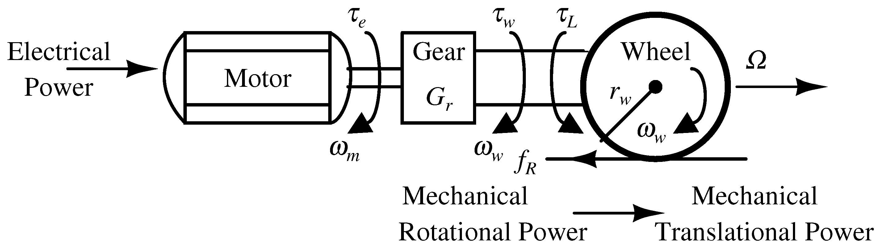
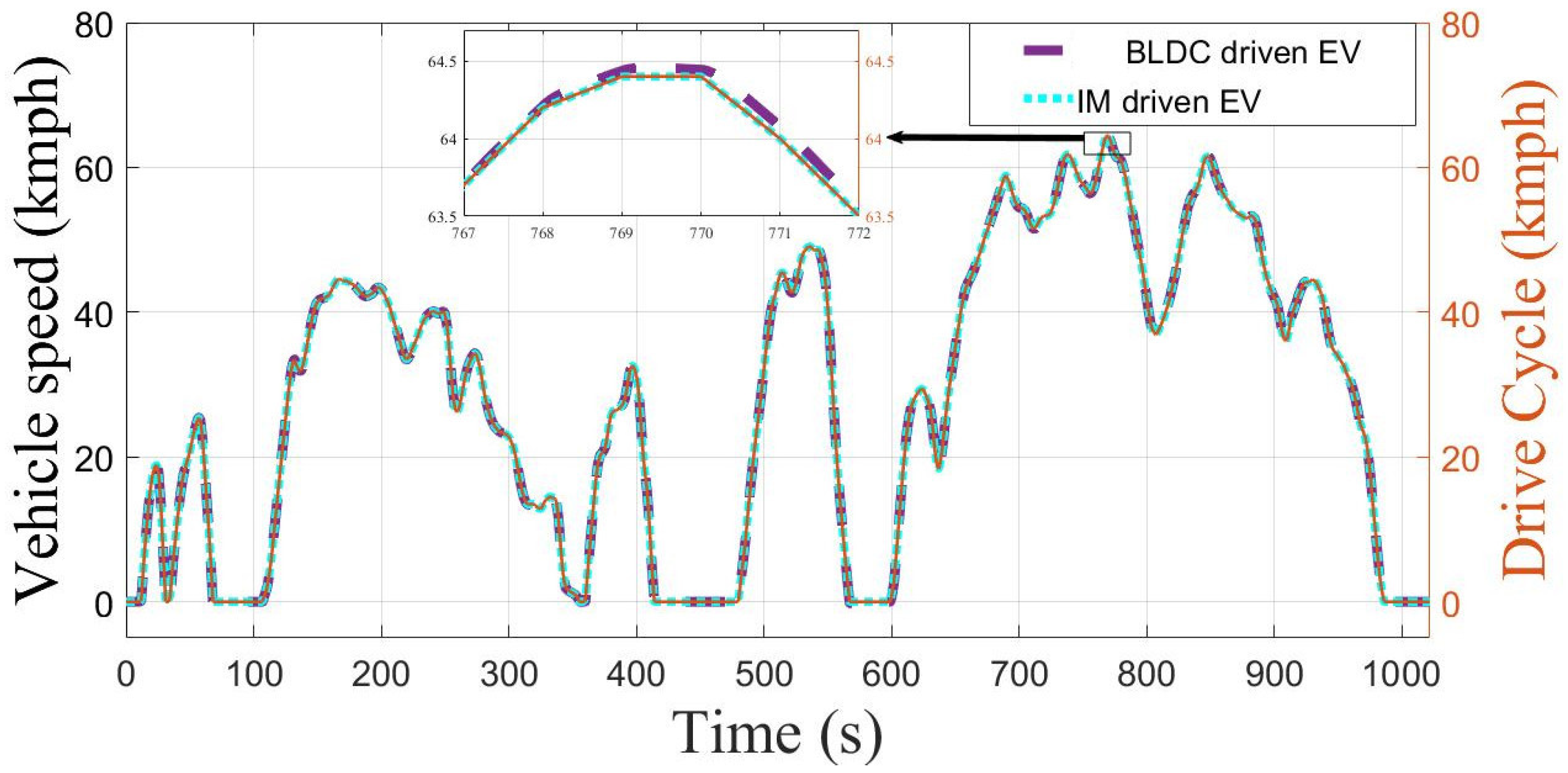
As the motor is coupled with the vehicle body, the mathematical model can be derived by using the coupled system altogether. The motor transforms the electrical power to mechanical power in the motor shaft, which is connected to the wheel of the vehicle through a transmission system consisting of a gear box, as shown in Figure 10. Using the developed electromagnetic torque from the motor (${\tau }_e$ for BLDC and ${\tau }_{\mathrm{em}}$ for IM), the wheel torque as well as the force exerted on the wheel are calculated. The wheel torque is responsible for generation of the tractive force $f_{\mathrm{tr}}$. By considering the transmission efficiency ($\eta$), the radius of wheel ($r_w$) and the gear ratio ($G_r$), the tractive torque or wheel torque (${\tau }_w$) and the tractive force ($f_{tr}$) supplied to the wheel are calculated as follows:

$${\tau }_w=\frac{\eta {\tau }_e}{G_r},f_{\mathrm{tr}}=\frac{{\tau }_w}{r_w}$$

(32)

The gear ratio can be described as a torque multiplier or speed reducer. Therefore, the rotational speed of the motor and rotational speed of the wheel of the vehicle are related by ${\omega }_w={\omega }_m{G}_r$. By neglecting the slipping of the running wheel, now the rotational speed of the wheel (${\omega }_w$) is transformed into the translational speed of the vehicle ($\mathsf{\Omega }$), and the acceleration force ($f_a$) can be calculated as follows:

$$\mathsf{\Omega }={\omega }_w{r}_w=\left({\omega }_m{G}_r\right)r_w,f_a=\delta m\frac{d\mathsf{\Omega }}{dt}=\delta m{r}_w\frac{d{\omega }_w}{dt}$$

(33)

It is worth noting that the transmission efficiency $\eta$ is not used for the speed conversion calculation. Moreover, the acceleration force ($f_a$) combines both the linear and rotational acceleration forces. In this context, the calculation of the rotational inertia factor ($\delta$) or mass factor is highly important. It requires the knowledge of the mass and distribution of the mass, form, position and dimensions of each rotating component within the vehicle, mainly the wheel and the rotor drive line of the motor. This is represented by [50]

$$\delta =1+\frac{I_w}{m{r}_w^2}+\frac{I_m{G}_r^2}{m{r}_w^2}$$

(34)

where $I_w$ and $I_m$ denote the total rotational inertia of the wheels and rotor drive line, respectively. As the vehicle could be all wheel drive, front wheel drive or rear wheel drive, the rotational inertia of the wheels and rotor drive line have almost the same values in motoring mode. But in the case of regenerating braking mode, it varies with the type of the drive [51]. In this study, a constant regeneration factor is used to simplify the analysis. Moreover, the rotational inertia is different for different vehicle types, depending on the number of wheels, coupling arrangements and gear ratio. If these values are not known, then the mass factor can be estimated using the following empirical relation [50]:

$$\delta =1+{\delta }_1+{\delta }_2{G}_r^2=1+0.04+0.0025G_r^2$$

(35)

Therefore, the equivalent mass ($\delta m$) is a function of the vehicle mass (m) and gear ratio ($G_r$). In this study, the effect of all the rotational inertia of the rotating components is considered by increasing the mass of the vehicle (m) by 1.05 times [50,52]. As shown in Figure 10, the load torque (${\tau }_L$) at the wheels is the sum of the resistive toque (${\tau }_R$) and the torque due to acceleration force (i.e., ($f_a{r}_w$)).

The tractive force ($f_{\mathrm{tr}}$) delivered to the wheel to move the vehicle can also be established from the torque equation calculated at the wheels by considering the equivalent rotational inertia ($J_{\mathrm{ew}}$) as follows [53]:

$$\begin{array}{ccc}\hfill {\tau }_w-{\tau }_R& =& J_{\mathrm{ew}}\frac{d{\omega }_w}{dt}\hfill \\ \hfill \Rightarrow \frac{\eta {\tau }_e}{G_r}-f_R{r}_w& =& \left(\delta m{r}_w^2\right)\frac{d}{dt}\left(\frac{\mathsf{\Omega }}{r_w}\right)\hfill \\ \hfill \Rightarrow \mathsf{\Omega }& =& \frac{1}{\delta m}\int \left(\frac{\eta {\tau }_e}{G_r{r}_w}-f_R\right)dt\hfill \end{array}$$

(36)

Therefore, a first-order differential equation is used to calculate the vehicle speed from the motor’s electromagnetic torque according to Equation (36).

3.6. Interaction among the Subsystems of the EV

It has been shown (Figure 2) that the EV powertrain is a nonlinear, dynamical integrated electromechanical system providing the power source for transportation. The interaction among different subsystems is important to reflect the EV’s dynamics on a mathematical framework, as shown in Figure 11. Therefore, starting from the battery and up to the vehicle dynamics, the steps in the analysis of the EV are as follows:

• The battery provides the terminal voltage ($v_b$) by solving Equations (1) and (2) using the parameters from

  Table A2. Battery specifications and parameters.

  Specification	Value	Parameter	Value
  Type	${\mathrm{LiFeO}}_4$	Internal resistance ($r_b$)	20 m$\mathsf{\Omega }$
  Voltage range	40–58.4 V	Nominal capacity ($Q_{\mathrm{bat}}$)	50 Ah
  Nominal energy	2.4 kWh	Battery nominal voltage ($V_{\mathrm{nb}}$)	48 V
  Cycle life (0.5C@25 ${}^{\circ }$C)	≥4000	Charge/discharge current ($I_b$)	60 A
  Max. discharge current ($I_{\mathrm{bp}}$)	100 A	Initial state of charge ($SoC\left(t_0\right)$)	100%
  		Battery efficiency (${\eta }_b$)	90%

  with the collected battery discharge current (Equation (3)) from the bidirectional DC-DC converter.
• Using Equations (3) and (4), the variables $i_L$ and $v_c$ of the bidirectional DC-DC converter are calculated with the component values from

  Table A3. Bidirectional DC-DC converter specifications and parameters.

  Specification	Value	Parameter	BLDC	IM
  Input voltage	40–58.4 V	Inductance (L)	200 µH	625  µH
  Current ripple	10%	ESR of inductor ($r_L$)	20 m$\mathsf{\Omega }$	60 m$\mathsf{\Omega }$
  DC-link voltage ripple	5%	Capacitance (C)	447 µF	247 µF
  Load	0–30 A	ESR of capacitor ($r_C$)	2 m$\mathsf{\Omega }$	5 m$\mathsf{\Omega }$
  		Switch on resistance ($r_{\mathrm{on}}$)	13.8 m$\mathsf{\Omega }$	13.8 m$\mathsf{\Omega }$
  		Switching frequency ($f_s$)	20 kHz	20 kHz

  and the switching signals provided by the DC-link voltage controller. These switching signals are generated by solving Equation (8) with the help of Equations (6) and (7). The control parameters are also given in

  Table A4. DC-link voltage controller parameters.

  Parameter	BLDC	IM
  DC-link voltage reference ($V_{\mathrm{ref}}$)	$3\mathrm{V}$	$5\mathrm{V}$
  Voltage feedback gain ($K_{\mathrm{fbv}}$)	1/32	1/44
  Current feedback gain ($K_{\mathrm{fbi}}$)	1/60	1/30
  Voltage loop proportional gain ($K_{\mathrm{pv}}$)	1	0.4
  Voltage loop integral gain ($K_{\mathrm{iv}}$)	200  s${}^{-1}$	100 s${}^{-1}$
  Current loop proportional gain ($K_{\mathrm{pi}}$)	0.5	0.2
  Current loop integral gain ($K_{\mathrm{ii}}$)	50 s${}^{-1}$	50 s${}^{-1}$
  Ramp amplitude ($V_M$)	1 V	1 V
  Current sensed resistance ($R_g$)	1 $\mathsf{\Omega }$	1 $\mathsf{\Omega }$

  . The variable $i_R$ acting on the DC link during motoring as well as regenerative braking is calculated from the power taken or given, respectively, by the motor.
• The DC-link voltage ($v_{\mathrm{dc}}$) is converted to three phase voltages in the inverter model by solving Equation (9) with the help of Equation (10), which needs six gate pulses from the speed controller. In the case of BLDC, the pulses are calculated as given in [43] using Equation (19) and

  Table A6. BLDC motor controller parameters.

  Parameter	Value
  Speed loop proportional gain ($K_{\mathrm{ps}}$)	10
  Speed loop integral gain ($K_{\mathrm{is}}$)	100  s${}^{-1}$
  Switching frequency ($f_s=1/T_s$)	20 kHz
  Sawtooth amplitude ($V_r$)	1 V

  . In the case of an IM, the pulses are calculated as given in [49] using Equations (25)–(30) and

  Table A8. Induction motor controller parameters.

  Parameter	Value
  Speed loop proportional gain ($K_{\mathrm{pim}}$)	100
  Speed loop integral gain ($K_{\mathrm{iim}}$)	50 s${}^{-1}$
  Torque hysteresis band ($h_{\tau }$)	0.1  Nm
  Flux hysteresis band ($h_{\psi }$)	0.01 Wb
  Flux reference (${\psi }_{\mathrm{ref}}$)	0.996 Wb

  .
• The three phase voltages from the inverter are fed to the two different motors to produce the electromagnetic torque (${\tau }_e$ for BLDC and ${\tau }_{\mathrm{em}}$ for the IM). In the case of a BLDC motor, this is calculated by solving Equations (12)–(17) using

  Table A5. BLDC motor specification and parameters.

  Specification	Value	Parameter	Value
  Rated power	3.3 kW	Stator resistance ($R_s$)	7 m$\mathsf{\Omega }$
  Rated torque	10 Nm	Stator inductance ($L_s$)	105 µH
  Rated speed	3200 rpm	Amplitude of flux linkage ($\lambda$)	0.031 Wb
  Rated voltage	96 V	Number of pole pair (p)	4
  Rated current	36 A	Back EMF constant and torque constant ($K_E=K_T$)	0.248 V-s/rad
  Peak torque	25 Nm	Rotor inertia (J)	0.009 kg-m${}^2$
  Working efficiency	90%	Viscous coefficient (B)	0.000302 Nm-s/rad

  , and for IM, this is calculated by solving Equations (20)–(27) using

  Table A7. Induction motor specifications and parameters.

  Specification	Value	Parameter	Value
  Rated power	3.7 kW	Stator resistance ($R_{\mathrm{sm}}$)	0.08 $\mathsf{\Omega }$
  Rated torque	50 Nm	Rotor resistance ($R_r$)	0.10 $\mathsf{\Omega }$
  Rated speed	710 rpm	Stator leakage inductance ($L_{\mathrm{sm}}$)	0.0073 H
  Rated voltage	220 V	Rotor leakage inductance ($L_r$)	0.0073 H
  Rated current	15 A	Magnetizing inductance ($L_m$)	0.93 H
  Peak torque	75 Nm	Number of pole pair ($p_m$)	4
  Working efficiency	85%	Rotor inertia ($J_m$)	0.09  kg-m${}^2$
  		Viscous coefficient ($B_m$)	0.000302 Nm-s/rad

  . The motor takes the rotor angular velocity (${\omega }_m$) from the vehicle model.
• The wheel torque (${\tau }_w$) is calculated using Equation (32). This provides the tractive force applied to the vehicle. Therefore, the angular velocity of the rotor (${\omega }_m$) is translated into the vehicle’s speed ($\mathsf{\Omega }$), which is calculated using Equation (36) with the help of

  Table A9. Two-wheeler vehicle parameters.

  Parameter	Value
  Gross vehicle weight (m)	200 kg
  Gravitational acceleration (g)	9.8 m/s${}^2$
  Rolling coefficient (${\mu }_{\mathrm{rr}}$)	0.006
  Drag coefficient ($C_D$)	$0.9$
  Air density ($\rho$)	1.2 kg/m${}^3$
  Vehicle frontal area ($A_f$)	0.6 m${}^2$
  Wheel radius ($r_w$)	0.28 m
  Slope of the road $\left(\theta \right)$	$0^{\circ }$
  Gear ratio $\left(G_r\right)$	1:5 (BLDC) and 1:1 (IM)
  Transmission efficiency ($\eta$)	0.8 (BLDC) and 0.8 (IM)

  .

4. State-Space Averaged and Small-Signal Models of the EV

For a BLDC motor-driven EV, the state-space averaged model is derived from the switched nonlinear model shown in Figure 11. The number of differential equations in each subsystem and the interactions among the subsystems can be clearly identified. Similarly, the state-space averaged model for the IM-driven EV can be derived. As the high-frequency switching signals are replaced by average value in terms of the duty ratios of the bidirectional DC-DC converter and the three-phase VSI $d_1$ and $d_2$ ($0\le d_1,d_2\le 1$), the ripple information in the waveforms is lost. The advantages of this model are that the overall dynamics are captured in less time compared with the switched model and a control-oriented small-signal model [54] can be derived. As the drive cycle is a time-varying reference, the system is analyzed at the worst case constant reference (64.4 km/h for WLTC Class 1) to obtain the steady state response. The small-signal model is derived by perturbing the state variables and the duty ratios around their steady state values. This model is particularly useful for selection of the controller parameters of the two-loop control for a bidirectional DC-DC converter and the motor control, as given in Table A4, Table A6 and Table A8. The powertrain parameters of each subsystem are designed as shown in the literature [55,56]. The following method has been used for the selection as well as tuning of the PI controller parameters. The small-signal transfer functions have been obtained for the two-loop controlled bidirectional DC-DC converter. The corresponding block diagram is shown in Figure 12. This diagram is obtained based on the control circuit diagram given in Figure 4. The loop gain of the two-loop controlled boost converter is calculated as follows:

$$T_{\mathrm{LG}}\left(s\right)=G_{\mathrm{cv}}\left(s\right)\left[\frac{G_{\mathrm{ci}}\left(s\right)G_{\mathrm{ramp}}\left(s\right)G_{\mathrm{id}}\left(s\right)}{1+G_{\mathrm{ci}}\left(s\right)G_{\mathrm{ramp}}\left(s\right)G_{\mathrm{id}}\left(s\right)H_i\left(s\right)}\right]G_{\mathrm{vi}}\left(s\right)H_v\left(s\right)$$

(37)

where $G_{\mathrm{vi}}\left(s\right)=\left(K_{\mathrm{pv}}+\frac{K_{\mathrm{iv}}}{s}\right)$, $G_{\mathrm{ci}}\left(s\right)=\left(K_{\mathrm{pi}}+\frac{K_{\mathrm{ii}}}{s}\right)$, $G_{\mathrm{ramp}}\left(s\right)=\frac{1}{V_M}$, $H_v\left(s\right)=K_{\mathrm{fbv}}$ and $H_i\left(s\right)=K_{\mathrm{fbi}}$. By neglecting all the parasitic elements, the transfer functions from the converter are calculated from the bidirectional DC-DC subsystem block in Figure 11:

$$G_{\mathrm{id}}\left(s\right)=\frac{{\widehat{i}}_L\left(s\right)}{{\widehat{d}}_1\left(s\right)}=\frac{\frac{I_L}{1-D_1}+\frac{sC{V}_{\mathrm{dc}}}{{(1-D_1)}^2}}{1+\frac{s^{2}LC}{{(1-D_1)}^2}},G_{\mathrm{vi}}\left(s\right)=\frac{{\widehat{v}}_{\mathrm{dc}}\left(s\right)}{{\widehat{i}}_L\left(s\right)}=\frac{\frac{V_{\mathrm{dc}}}{L}-\frac{sL}{1-D_1}}{1+\frac{sC{V}_{\mathrm{dc}}}{I_L(1-D_1)}}$$

(38)

where $I_L$ and $D_1$ are the steady state inductor current and duty ratio, respectively. The closed-loop transfer function is given by

$$\frac{H_v.{\widehat{v}}_{\mathrm{ref}}}{{\widehat{v}}_{\mathrm{dc}}}=\frac{T_{\mathrm{LG}}\left(s\right)}{1+T_{\mathrm{LG}}\left(s\right)}$$

(39)

The Bode plot of the loop gain (gain margin = 3.52 dB and phase margin = 39.1${}^{\circ }$) and the step response of the closed-loop transfer function of the boost converter (rise time = 0.9 ms, maximum overshoot = 11.9% and settling time = 13.1 ms) are shown in Figure 13 and Figure 14, respectively. By tuning or adjusting the values of the PI controller gains, the desired gain and phase margins can be achieved. This analysis can be extended to other subsystems of the EV for tuning the controller gains [57]. There are sophisticated small-signal analysis tools [58,59] for the switched model which are not used in this paper.

5. Performance Evaluation Using the Switched and Averaged Models

The switched nonlinear model of the complete two-wheeler EV (Figure 2) was simulated with two different motors, namely a single-loop speed-controlled BLDC and DTC IM for the speed tracking of the WLTC Class 1 drive cycle. This simulation was performed on an automatically controlled two-wheeler EV while considering two modes of operation: motoring and regenerative braking. Comparison of the performances of the two motors and controllers is not performed in this paper.

5.1. Two-Wheeler EV with a BLDC Motor

The BLDC motor was controlled using a single-loop speed controller (Figure 7), and the speed tracking performance is shown in Figure 15.

The DC-link voltage (96 V ± 5% ripple) and the battery discharge current during the drive cycle (Figure 16) are the key parameters for the motor performance and battery stress observation, respectively. As shown in the inset of Figure 16, due to the switching in the switched nonlinear model, transition spikes and steady state ripples were clearly observed throughout the drive cycle. The state-space averaged model performed the simulation with a substantially reduced computation time at the price of losing ripple information.

The torque delivered to the transmission system by the BLDC motor is shown in Figure 17. It is interesting to note that while tracking the drive cycle, spikes were inevitable during the transitions between idling, the steady state, acceleration and deceleration. But the magnitude of the spikes could vary with the topology and controller used in the EV.

The most important advertising factor of an EV is the SoC, which is shown in Figure 18. The end point of the SoC of the battery calculation for a drive cycle is required for obtaining the range of the EV, as shown below:

$$\begin{array}{ccc}\hfill \mathrm{range}\mathrm{of}\mathrm{EV}/\mathrm{charge}& =& \frac{\mathrm{available}\mathrm{energy}\mathrm{of}\mathrm{battery}}{\mathrm{energy}\mathrm{required}\mathrm{by}\mathrm{EV}\mathrm{per}\mathrm{km}}\hfill \\ \hfill \Rightarrow \mathrm{range}\mathrm{of}\mathrm{EV}/\mathrm{charge}& =& \frac{(V_{\mathrm{nb}}\times Q_{\mathrm{bat}}\times {\eta }_b)}{\left(\frac{\mathrm{energy}\mathrm{consumed}\mathrm{by}\mathrm{EV}}{\mathrm{total}\mathrm{distance}\mathrm{covered}\mathrm{in}\mathrm{km}}\right)}=\frac{(V_{\mathrm{nb}}\times Q_{\mathrm{bat}}\times {\eta }_b)}{\left[\frac{\left(1-\frac{\%\mathrm{SoC}\mathrm{at}\mathrm{end}}{100}\right)\times V_{\mathrm{nb}}{Q}_{\mathrm{bat}}}{\mathrm{total}\mathrm{distance}\mathrm{covered}\mathrm{in}\mathrm{km}}\right]}\hfill \end{array}$$

(40)

where ${\eta }_b$ is the battery’s capability to transfer energy from the input of the battery to the output. For example, if 2.4 kWh is stored in the battery while charging, then one can effectively retrieve only 2.16 kWh while discharging. Therefore, the round trip efficiency of the battery is 90%. When considering 90% battery efficiency $\left({\eta }_b\right)$ and a regeneration factor of 20% during regenerative braking throughout the drive cycle, the selected BLDC motor-driven two-wheeler provides a range of 121.365 km/charge. For this calculation, the percentage of SoC at the end of the WLTC class 1 drive cycle (Table A1) is used from Figure 18, which is 94. The inset of Figure 18 shows that during regenerative braking, the battery was charging for both cases.

5.2. Comparison of Simulation Time with the Commercial Software MATLAB- and Simulink-Based EV Model

In the commercial software of matlab’s Simulink R2023b, the overall EV switched model was built by combining the built-in components, such as the inductor, capacitor, switch and diode, for the bidirectional DC-DC converter, two-loop DC-link voltage controller and the three-leg, six-switch inverter. Nonidealities such as the ESR and on switch resistance were also selected accordingly. The battery model (look-up table-based), BLDC motor and two-wheeler vehicle dynamics were available in Simscape, which helped to simulate multi-domain physical systems within matlab’s Simulink environment. The tabulated battery model from the Simscape is used to match a characteristic directly from a datasheet. It can be used to represent any battery chemistry. A brushless DC (BLDC) motor was implemented using a permanent magnet synchronous motor (PMSM). The hall sensors and commutation logic (motoring and braking) were also implemented. The two-wheeler vehicle dynamics included built-in simulation blocks, which were the simple gear, the two tires and the vehicle body. In this modeling, instead of considering the wheel inertia, the externally defined additional mass parameter was set to the on position (inside the vehicle body) to include an additional 5% mass, as considered in this paper. The parameters for the other subsystems were taken from the parameter tables.

In the proposed equation-based model, the state variables are governed by differential equations, and switching conditions are formed using an algebraic equation. To test the performance of the equation-based switched model given in the paper with the switched model developed in the commercial software matlab and Simulink, a 5 s drive cycle was developed as shown in Figure 19.

This 5 s drive cycle consists of 0.5 s of idling, 2 s of acceleration at 0.75 m/s${}^2$, 1 s of a constant speed of 5.4 km/h and 1.5 s of deceleration at −1 m/s${}^2$. Both models follow the drive cycle extremely closely, with errors of less than 0.5%. The simulation is run by a desktop with the following configuration: an Intel (R) Core i5-10500 CPU@3.1 GHz processor, 3096 MHz, 6 core(s), 12 logical processors, 64-bit system, x64-based processor and 16 GB of installed RAM.

The proposed equation-based modeling technique took 112 s for the 5 s drive cycle for the switched model. In the case of matlab and Simulink model, the simulation was completed in 292 s. For running the simulation in matlab and Simulink, there are three modes: normal, accelerator and rapid accelerator. In the simulation, the accelerator mode was used. For both compared models, a 1 µs step size was considered. With the used switching frequency of 20 kHz (switching period = 50 µs), 50 samples were taken within a switching period. Similarly, in the case of the state-space averaged model, the proposed technique took 12 s with a 25 µs step size. The simulation step size in this case was selected from the natural period of the converter and inverter (whichever one was smaller). From the calculation, we found 25 µs (i.e., two samples were taken within a switching period of 50 µs). In matlab and Simulink, a similar averaged model was developed using the built-in average value switch module for the converter and the inverter for the design of the overall EV. This average value switch module was based on the equivalent circuit model of the switch using the dependent (controlled) voltage and current sources. This is also called circuit averaging or averaged switch modeling. This technique also yields equivalent results, but the derivation involves manipulation of a circuit rather than equations. This matlab and Simulink model took 22 s to complete the process.

5.3. Two-Wheeler EV with an Induction Motor

The speed tracking response of the EV with an IM-driven transmission system is shown in Figure 15. The DC-link voltage (220 V) and the battery discharge current can be observed in Figure 20. The average value of the battery discharge current was the same in both models (BLDC- and IM-driven EVs) as the power requirement to drive the vehicle was the same. The electromagnetic torque generated by the IM subsystem is shown in Figure 21. The range was also calculated for this EV while observing the SoC at the end to be 94.06 (Figure 18), which was 122.6 km/charge using Equation (40).

5.4. Short-Term Simulation for the DTC IM Two-Wheeler EV

To check the performance of each subsystem of the EV, a short time drive cycle was constructed. In this drive cycle (164 s), the idle time, acceleration (0.226 m/s${}^2$) time, constant speed (64.4 km/h) time and deceleration (0.226 m/s${}^2$) time were 1 s, 79 s, 5 s and 79 s, respectively.

As shown in Figure 22, the battery terminal voltage monotonically decreased as the vehicle accelerated. Then, the terminal voltage increased at the transition to the constant speed phase. In this phase, the terminal voltage decreased slowly, but at the decelerating phase, the terminal voltage continuously increased due to the regenerative braking. Due to the low regeneration factor of 20%, only a small amount of energy was fed back to the battery.

In the case of the bidirectional DC-DC converter, the inductor current (Figure 23) increased during the acceleration phase of the vehicle due to the increasing demand of the torque of the motor. At a constant speed, the current was also constant, but during the deceleration phase, the average current started decreasing and even became negative (i.e., charging the battery). In the inset of Figure 23, the inductor current and DC-link voltage waveforms are shown for 10 switching cycles at a constant speed.

In Figure 24, the waveforms of the three phase voltages of the inverter at a constant speed are shown. According to the switching signals of the six switches, the phase voltages were determined.

Similar to the inductor current of the bidirectional DC-DC converter, the electromagmetic torque (Figure 25) increased during the acceleration phase of the vehicle due to the increasing demand of the torque of the motor. At a constant speed, the torque was also constant, but then the torque started decreasing and even became negative.

To check the performance of the DTC, the locus of the direct and quadrature axis fluxes were drawn in the state-space as shown in Figure 26.

6. Conclusions

In this paper, a general mathematical framework for EVs was developed using a switched nonlinear model. Different motors with controllers were used for two-wheelers, keeping all other subsystems such as the battery, DC-DC bidirectional converter, inverter and vehicle body fixed. Due to the small time step, this model captured the essential switching dynamics. It is interesting to note that this equation-based switched model took less simulation time compared with the other module-based EV model available in commercial software. This switched model also considers the nonidealities of the system and interaction among subsystems and is applicable for all operating conditions (e.g., motoring and regenerative braking). The averaged model and a small signal model were derived from the switching model for capturing long-term behavior and selecting the controller parameters, respectively.

The switched model and averaged model are used for the performance measures of an EV (i.e., the tracking of the drive cycle, SoC of the battery, battery discharge current, DC-link voltage and motor torque waveforms). This general mathematical framework can be extended to multiple sources, different converter topologies, motor drives and their controllers and different vehicle bodies (e.g., four-wheeler, bus or truck) with a more realistic subsystem model of the overall EV. The advanced optimal control algorithms can be tested in this model. Moreover, the switched model can be useful for identifying different types of instabilities related to the nonlinear switching dynamics with variation in the disturbance parameters.

References

1. Ehsani, M.; Singh, K.V.; Bansal, H.O.; Mehrjardi, R.T. State of the art and trends in electric and hybrid electric vehicles. Proc. IEEE 2021, 109, 967–984. [Google Scholar] [CrossRef]
2. Mo, T.; Li, Y.; tak Lau, K.; Poon, C.K.; Wu, Y.; Luo, Y. Trends and emerging technologies for the development of Electric Vehicles. Energies 2022, 15, 6271. [Google Scholar] [CrossRef]
3. Amrhein, M.; Krein, P.T. Dynamic simulation for analysis of hybrid electric vehicle system and subsystem interactions, including power electronics. IEEE Trans. Veh. Technol. 2005, 54, 825–836. [Google Scholar] [CrossRef]
4. Adegbohun, F.; von Jouanne, A.; Phillips, B.; Agamloh, E.; Yokochi, A. High Performance Electric Vehicle Powertrain Modeling, Simulation and Validation. Energies 2021, 14, 1493. [Google Scholar] [CrossRef]
5. Butler, K.L.; Ehsani, M.; Kamath, P. A Matlab-based modeling and simulation package for electric and hybrid electric vehicle design. IEEE Trans. Veh. Technol. 1999, 48, 1770–1778. [Google Scholar] [CrossRef] [Green Version]
6. Vidal-Bravo, S.; De La Cruz-Soto, J.; Arrieta Paternina, M.R.; Borunda, M.; Zamora-Mendez, A. Light electric vehicle powertrain: Modeling, simulation, and experimentation for engineering students using PSIM. Comput. Appl. Eng. Educ. 2020, 28, 406–419. [Google Scholar] [CrossRef]
7. Mousazadeh, H.; Keyhani, A.; Javadi, A.; Mobli, H.; Abrinia, K.; Sharifi, A. Design, simulation and construction of two synchronized DC motors’ driver for EVs. In Proceedings of the WSEAS International Conference on Mathematics and Computers in Science and Engineering, Rodos, Greece, 22–24 July 2009; pp. 19–24. [Google Scholar]
8. Kumar, R.; Saxena, R.; Srivastava, A. Modeling, simulation and energy-flow study of a battery electric vehicle in Labview. In Proceedings of the 2019 IEEE International Conference on Electrical, Computer and Communication Technologies (ICECCT), Tamil Nadu, India, 20–22 February 2019; IEEE: Piscataway Township, NJ, USA, 2019; pp. 1–7. [Google Scholar]
9. Cole, G. SIMPLEV: A Simple Electric Vehicle Simulation Program, Version 1.0; Technical Report; EG and G Idaho, Inc.: Idaho Falls, ID, USA, 1991. [Google Scholar]
10. Wipke, K.B.; Cuddy, M.R.; Burch, S.D. ADVISOR 2.1: A user-friendly advanced powertrain simulation using a combined backward/forward approach. IEEE Trans. Veh. Technol. 1999, 48, 1751–1761. [Google Scholar] [CrossRef]
11. Rahman, Z.; Butler, K.; Ehsani, M. Designing parallel hybrid electric vehicles using V-ELPH 2.01. In Proceedings of the 1999 American Control Conference (Cat. No. 99CH36251), San Diego, CA, USA, 2–4 June 1999; IEEE: Piscataway Township, NJ, USA, 1999; Volume 4, pp. 2693–2697. [Google Scholar]
12. Markel, T.; Brooker, A.; Hendricks, T.; Johnson, V.; Kelly, K.; Kramer, B.; O’Keefe, M.; Sprik, S.; Wipke, K. ADVISOR: A systems analysis tool for advanced vehicle modeling. J. Power Sources 2002, 110, 255–266. [Google Scholar] [CrossRef]
13. Jones-Jackson, S.; Rodriguez, R.; Yuhang Yang, L.L.; Emadi, A. Overview of current thermal management of automotive power electronics for traction purposes and future directions. IEEE Trans. Transp. Electrif. 2022, 8, 2412–2428. [Google Scholar] [CrossRef]
14. Liu, W.; Placke, T.; Chau, K. Overview of batteries and battery management for electric vehicles. Energy Rep. 2022, 8, 4058–4084. [Google Scholar] [CrossRef]
15. Kotb, R.; Chakraborty, S.; Tran, D.D.; Abramushkina, E.; Baghdadi, M.E.; Hegazy, O. Power electronics converters for electric vehicle auxiliaries: State of the art and future trends. Energies 2023, 16, 1753. [Google Scholar] [CrossRef]
16. Klerk, M.L.D.; Saha, A.K. A comprehensive review of advanced traction motor control techniques suitable for electric vehicle applications. IEEE Access 2021, 9, 125080–125108. [Google Scholar] [CrossRef]
17. Yang, G.; Yao, J.; Dong, Z. Neuroadaptive learning algorithm for constrained nonlinear systems with disturbance rejection. Int. J. Robust Nonlinear Control 2022, 32, 6127–6147. [Google Scholar] [CrossRef]
18. Yang, G. Asymptotic tracking with novel integral robust schemes for mismatched uncertain nonlinear systems. Int. J. Robust Nonlinear Control 2023, 33, 1988–2002. [Google Scholar] [CrossRef]
19. Wang, Z.; Ching, T.W.; Huang, S.; Wang, H.; Xu, T. Challenges faced by electric vehicle motors and their solutions. IEEE Access 2020, 9, 5228–5249. [Google Scholar] [CrossRef]
20. Karki, A.; Phuyal, S.; Tuladhar, D.; Basnet, S.; Shrestha, B.P. Status of pure electric vehicle power train technology and future prospects. Appl. Syst. Innov. 2020, 3, 35. [Google Scholar] [CrossRef]
21. Hamada, A.T.; Orhan, M.F. An overview of regenerative braking systems. J. Energy Storage 2022, 52, 105033. [Google Scholar] [CrossRef]
22. Saha, S.; Nishanth, M.; Praveen, T.; Rajalekshmi, N.; Prabu, T. Comparative analysis between direct torque control and v/f control for electric vehicles. In Proceedings of the 2020 11th International Conference on Computing, Communication and Networking Technologies (ICCCNT), Kharagpur, India, 1–3 July 2020; IEEE: Piscataway Township, NJ, USA, 2020; pp. 1–6. [Google Scholar]
23. Lipu, M.S.H.; Faisal, M.; Ansari, S.; Hannan, M.A.; Karim, T.F.; Ayob, A.; Hussain, A.; Miah, M.S.; Saad, M.H.M. Review of electric vehicle converter configurations, control schemes and optimizations: Challenges and suggestions. Energies 2021, 10, 477. [Google Scholar] [CrossRef]
24. Hassan, M.; Mossa, M.; Dousoky, G. Evaluation of electric dynamic performance of an electric vehicle system using different control techniques. Electronics 2021, 10, 2586. [Google Scholar] [CrossRef]
25. Teoh, J.X.; Stella, M.; Chew, K.W. Performance analysis of electric vehicle in worldwide harmonized light vehicles test procedure via vehicle simulation models in ADVISOR. In Proceedings of the 2019 IEEE 9th International Conference on System Engineering and Technology (ICSET), Shah Alam, Malaysia, 7 October 2019; IEEE: Piscataway Township, NJ, USA, 2019; pp. 215–220. [Google Scholar]
26. Addendum 15: Global Technical Regulation No. 15. Worldwide Harmonized Light Vehicles Test Procedure; UNECE: Geneva, Switzerland, 2015.
27. Buchmann, I. Batteries in a Portable World—A Handbook on Rechargeable Batteries for Non-Engineers; Cadex Electronics Inc.: Richmond, BC, Canada, 2016. [Google Scholar]
28. Fotouhi, A.; Auger, D.J.; Propp, K.; Longo, S.; Wild, M. A review on electric vehicle battery modelling: From Lithium-ion toward Lithium–Sulphur. Renew. Sustain. Energy Rev. 2016, 56, 1008–1021. [Google Scholar] [CrossRef] [Green Version]
29. Campagna, N.; Castiglia, V.; Miceli, R.; Mastromauro, R.A.; Spataro, C.; Trapanese, M.; Viola, F. Battery models for battery powered applications: A comparative study. Energies 2020, 13, 4085. [Google Scholar] [CrossRef]
30. Cao, Y.; Kroeze, R.C.; Krein, P.T. Multi-timescale parametric electrical battery model for use in dynamic electric vehicle simulations. IEEE Trans. Transp. Electrif. 2016, 2, 432–442. [Google Scholar] [CrossRef]
31. Wang, Q.; Gao, T.; Li, X. SOC estimation of lithium-ion battery based on equivalent circuit model with variable parameters. Energies 2022, 15, 5829. [Google Scholar] [CrossRef]
32. Tran, M.K.; DaCosta, A.; Mevawalla, A.; Panchal, S.; Fowler, M. Comparative study of equivalent circuit models performance in four common Lithium-Ion batteries: LFP, NMC, LMO, NCA. Batteries 2021, 7, 51. [Google Scholar] [CrossRef]
33. Potrykus, S.; Kutt, F.; Nieznański, J.; Morales, F.J.F. Advanced lithium-ion battery model for power system performance analysis. Energies 2020, 13, 2411. [Google Scholar] [CrossRef]
34. Wang, Z.; Feng, G.; Zhen, D.; Gu, F.; Ball, A. A review on online state of charge and state of health estimation for lithium-ion batteries in electric vehicles. Energy Rep. 2021, 7, 5141–5161. [Google Scholar] [CrossRef]
35. Tremblay1, O.; Dessaint, L.A. Experimental validation of a battery dynamic model for EV applications. In Proceedings of the EVS24 International Battery, Hybrid and Fuel Cell Electric Vehicle Symposium, Stavanger, Norway, 13–16 May 2009; pp. 289–298. [Google Scholar]
36. Available online: https://www.solacity.com/how-to-keep-lifepo4-lithium-ion-batteries-happy/ (accessed on 20 July 2023).
37. Erickson, R.W.; Maksimovic, D. Fundamentals of Power Electronics; Springer Science & Business Media: Berlin/Heidelberg, Germany, 2007. [Google Scholar]
38. Lee, B.K.; Ehsani, M. A simplified functional simulation model for three-phase voltage-source inverter using switching function concept. IEEE Trans. Ind. Electron. 2001, 48, 309–321. [Google Scholar]
39. Yildirim, M.; Polat, M.; Kürüm, H. A survey on comparison of electric motor types and drives used for electric vehicles. In Proceedings of the 2014 16th International Power Electronics and Motion Control Conference and Exposition, Antalya, Turkey, 21–24 September 2014; IEEE: Piscataway Township, NJ, USA, 2014; pp. 218–223. [Google Scholar]
40. Liu, C.; Chau, K.; Lee, C.H.; Song, Z. A critical review of advanced electric machines and control strategies for electric vehicles. Proc. IEEE 2020, 109, 1004–1028. [Google Scholar] [CrossRef]
41. Sreejith, R.; Rajagopal, K.; Singh, B. Modelling and analysis of PMBLDC motor based three wheeler EV for closed loop optimum operation. In Proceedings of the 2016 IEEE International Conference on Power Electronics, Drives and Energy Systems (PEDES), Trivandrum, India, 14–17 December 2016; IEEE: Piscataway Township, NJ, USA, 2016; pp. 1–5. [Google Scholar]
42. Catata, E.O.H.; dos Santos Neto, P.J.; Barros, T.A.S.; Filho, E.R. Modeling, control and regenerative braking of BLDC machines in electric bycicles. In Proceedings of the Congresso Brasileiro de Automática-CBA, Virtual Event, 23–26 November 2020; Volume 2. [Google Scholar]
43. Lee, S.; Lemley, T.; Keohane, G. A comparison study of the commutation methods for the three-phase permanent magnet brushless DC motor. In Proceedings of the Electrical Manufacturing Technical Conference 2009: Electrical Manufacturing and Coil Winding Expo, EMCWA, Nashville, TN, USA, 29 September–1 October 2009; pp. 49–55. [Google Scholar]
44. Jääskeläinen, E.; Pohjalainen, P. DTC A Motor Control Technique for All Seasons; Technical Report; ABB: Zurich, Switzerland, 2015. [Google Scholar]
45. Kumar, R.H.; Iqbal, A.; Lenin, N.C. Review of recent advancements of direct torque control in induction motor drives—A decade of progress. IET Power Electron. 2018, 11, 1–15. [Google Scholar] [CrossRef]
46. Alsofyani, I.M.; Idris, N.R.N.; Lee, K.B. Dynamic Hysteresis Torque Band for Improving the Performance of Lookup-Table-Based DTC of Induction Machines. IEEE Trans. Power Electron. 2018, 33, 7959–7970. [Google Scholar] [CrossRef]
47. Sutikno, T.; Idris, N.R.N.; Jidin, A.; Cirstea, M.N. An Improved FPGA Implementation of Direct Torque Control for Induction Machines. IEEE Trans. Ind. Inform. 2013, 9, 1280–1290. [Google Scholar] [CrossRef]
48. Mohan, N. Advanced Electric Drives: Analysis, Control, and Modeling Using MATLAB/Simulink®; John Wiley & Sons, Inc.: Hoboken, NJ, USA, 2014. [Google Scholar]
49. Reza, C.; Islam, M.D.; Mekhilef, S. A review of reliable and energy efficient direct torque controlled induction motor drives. Renew. Sustain. Energy Rev. 2014, 37, 919–932. [Google Scholar] [CrossRef]
50. Ehsani, M.; Gao, Y.; Gay, S.E.; Emadi, A. Modern Electric, Hybrid Electric, and Fuel Cell Vehicles: Fundamentals, Theory, and Design; CRC Press: Boca Raton, FL, USA, 2005. [Google Scholar]
51. Lee, J.; Nelson, D.J. Rotating inertia impact on propulsion and regenerative braking for electric motor driven vehicles. In Proceedings of the 2005 IEEE Vehicle Power and Propulsion Conference, Chicago, IL, USA, 7–9 September 2005; IEEE: Piscataway Township, NJ, USA, 2005; pp. 308–314. [Google Scholar]
52. Larminie, J.; Lowry, J. Electric Vehicle Technology Explained; John Wiley & Sons: Hoboken, NJ, USA, 2012. [Google Scholar]
53. Fajri, P.; Prabhala, V.A.K.; Ferdowsi, M. Emulating On-Road Operating Conditions for Electric-Drive Propulsion Systems. IEEE Trans. Energy Convers. 2016, 31, 1–11. [Google Scholar] [CrossRef]
54. Raga, C.; Lázaro, A.; Barrado, A.; Martín-Lozano, A.; Quesada, I. Step-by-step small-signal modeling and control of a light hybrid electric vehicle propulsion system. Energies 2019, 12, 4082. [Google Scholar] [CrossRef] [Green Version]
55. Maksimovic, D. Power Electronics for Electric Drive Vehicles; Technical Report; Power Electronics Seminar at IIT Kharagpur: Kharagpur, India, 2016. [Google Scholar]
56. Jhunjhunwala, A.; Kaur, P.; Jha, K.K.; Kannan, L. Fundamentals of Electric Vehicles: Technology & Economics, IIT Madras. Available online: https://nptel.ac.in/courses/108106170 (accessed on 20 July 2023).
57. Chauhan, A.; Mandal, K.; Panda, A. Performance improvement of electric vehicle using reset switch and bias. IFAC-PapersOnLine 2022, 55, 144–149. [Google Scholar] [CrossRef]
58. Mandal, K.; Banerjee, S.; Chakraborty, C. A new algorithm for small-signal analysis of DC-DC converters. IEEE Trans. Ind. Informatics 2014, 10, 628–636. [Google Scholar] [CrossRef]
59. Al-Turki1, Y.; El Aroudi, A.; Mandal, K.; Giaouris, D.; Abusorrah, A.; Hindawi, M.A.; Banerjee, S. Non-averaged cntrol-oriented modeling and relative stability analysis of DC-DC switching converters. Int. J. Circuit Theory Appl. 2018, 46, 565–580. [Google Scholar] [CrossRef]
Figure 1. Interconnection of different subsystems of an EV through a block diagram.
Electronics 12 03173 g001
Figure 2. The powertrain and control stage block diagram of the EV. Different subsystems are shown with dashed squares.
Electronics 12 03173 g002
Figure 3. The battery v oc vs. SoC curve and table of the battery from the manufacturer’s datasheet [36].
Electronics 12 03173 g003
Figure 4. Two-loop control for the DC-link voltage of the bidirectional DC-DC converter. The limiters are used for compensation of the integrator wind-up problem of the PI compensators.
Electronics 12 03173 g004
Figure 5. Circuit diagram of a three-phase VSI with a star-connected balanced load. For different motors, the load ( Z 1 , Z 2 and Z 3 ) will be replaced by the stator circuit of the motor. The two capacitors are used for analysis purposes.
Electronics 12 03173 g005
Figure 6. The equivalent circuit diagram of the stator winding of a BLDC motor.
Electronics 12 03173 g006
Figure 7. Schematic diagram of single-loop speed controller for BLDC motor.
Electronics 12 03173 g007
Figure 8. The d q -winding equivalent circuit of an induction motor (IM) in a stationary reference frame. The stationary d axis is aligned with the a axis of the stator.
Electronics 12 03173 g008
Figure 9. Schematic diagram of direct torque control (DTC) of an induction motor (IM).
Electronics 12 03173 g009
Figure 10. The rotor of the motor to the wheel of the vehicle dynamics and power flow through the gear box.
Electronics 12 03173 g010
Figure 11. State-space averaged model of an EV with a single-loop speed-controlled BLDC motor. The feedback gains are omitted for simplicity.
Electronics 12 03173 g011
Figure 12. Transfer function block diagram of two-loop controlled bidirectional DC-DC converter in boost mode. The small letter ’s’ denotes the Laplace variable.
Electronics 12 03173 g012
Figure 13. The Bode plot of the loop gain of the two-loop controlled DC-DC boost converter with I L = 36 A. Other parameters are given in Table A3 and Table A4.
Electronics 12 03173 g013
Figure 14. Step response of closed-loop boost converter.
Electronics 12 03173 g014
Figure 15. The speed tracking performance of BLDC- and IM-driven two-wheeler vehicles for the WLTC Class 1 drive cycle.
Electronics 12 03173 g015
Figure 16. Waveforms of the DC-link voltage (blue) and the battery discharge current (using the switched nonlinear model (purple) and the averaged model (green)) for the single-loop speed-controlled BLDC motor-driven EV.
Electronics 12 03173 g016
Figure 17. The electromagnetic torque delivered by BLDC (using the switched nonlinear model (blue) and the averaged model (green)) to the vehicle while tracking the WLTC Class 1 drive cycle.
Electronics 12 03173 g017
Figure 18. The SoC of the battery over the WLTC Class 1 drive cycle for the BLDC motor-driven EV (blue) and IM motor-driven EV (pink).
Electronics 12 03173 g018
Figure 19. Tracking performance of the proposed model (BLDC) and Simulink model (BLDC) for a 5 s drive cycle.
Electronics 12 03173 g019
Figure 20. Waveforms of the DC-link voltage (blue) and the battery discharge current (using the switched nonlinear model (purple) and the averaged model (green)) for the DTC-controlled IM-driven EV.
Electronics 12 03173 g020
Figure 21. Electromagnetic torque delivered by the IM to the vehicle while tracking the WLTC Class 1 drive cycle.
Electronics 12 03173 g021
Figure 22. The battery terminal voltage over the newly constructed drive cycle.
Electronics 12 03173 g022
Figure 23. The inductor current and DC-link voltage over the constructed drive cycle.
Electronics 12 03173 g023
Figure 24. The three phase voltages at a steady state at 80 s with a 64.4 km/h speed in the constructed drive cycle.
Electronics 12 03173 g024
Figure 25. The electromagnetic torque over the constructed drive cycle.
Electronics 12 03173 g025
Figure 26. The evolution of the d q fluxes in the state-space for the constructed drive cycle.
Electronics 12 03173 g026
Disclaimer/Publisher’s Note: The statements, opinions and data contained in all publications are solely those of the individual author(s) and contributor(s) and not of MDPI and/or the editor(s). MDPI and/or the editor(s) disclaim responsibility for any injury to people or property resulting from any ideas, methods, instructions or products referred to in the content.