Q-Learning and Efficient Low-Quantity Charge Method for Nodes to Extend the Lifetime of Wireless Sensor Networks

Abstract

With the rapid development of the Internet of Things (IoT), improving the lifetime of nodes and networks has become increasingly important. Most existing medium access control protocols are based on scheduling the standby and active periods of nodes and do not consider the alarm state. This paper proposes a Q-learning and efficient low-quantity charge (QL-ELQC) method for the smoke alarm unit of a power system to reduce the average current and to improve the lifetime of the wireless sensor network (WSN) nodes. Quantity charge models were set up, and the QL-ELQC method is based on the duty cycle of the standby and active times for the nodes and considers the relationship between the sensor data condition and the RF module that can be activated and deactivated only at a certain time. The QL-ELQC method effectively overcomes the continuous state–action space limitation of Q-learning using the state classification method. The simulation results reveal that the proposed scheme significantly improves the latency and energy efficiency compared with the existing QL-Load scheme. Moreover, the experimental results are consistent with the theoretical results. The proposed QL-ELQC approach can be applied in various scenarios where batteries cannot be replaced or recharged under harsh environmental conditions.

1. Introduction

Internet of Things (IoT) technology enables machines, such as home appliances, medical equipment, and industrial instruments, to interact with users and other machines via the Internet [1]. Wireless sensor networks (WSNs) are a broad category of IoT applications. WSNs can send and receive data via the Internet using a sink node [2,3]. The successful operation of a power system requires the support of communication networks with massive node access and latency-critical two-way reliable transmission [4]. However, power management in WSNs poses a significant challenge when the WSN must operate continuously for sustained periods without a consistent power source. In such contexts, the nodes have specific limitations regarding their memory, processing capacity, radio communication range, and energy supply [5]. One type of node uses batteries that cannot be replaced or recharged under harsh environmental conditions [6].

Although many complex communication protocols and routing algorithms have been proposed for WSNs, disadvantages, such as power dissipation, network complexity, and high costs, must be overcome for hardware and software implementation [7]. For long-term operation, the power-constrained condition is strict and limited, and a back-end circuit system is required to obtain the sensor information and to transmit the acquired data [8]. As the network scales up and the number of nodes increases, certain fundamental problems, such as energy-efficient data transmission, scalability, data gathering, and aggregation, become concerns [9]. Thus, an effective low-power circuit system is indispensable to ensure the long-term operation of WSNs [10,11,12]. To improve the WSN’s lifetime, the high-coverage communication of targets must be ensured before performing a sensor-node duty cycle [13,14]. The Cooperative Medium Access Control (C-MAC) [15] method for improving the duty cycle-based MAC with idle listening has been proposed. However, an additional channel is required to synchronize the nodes which consume additional energy.

Recently, reinforcement learning (RL) has been widely employed to address resource management problems in next-generation wireless networks [16]. The Q-learning technique is an RL approach in which the algorithm continuously learns by interacting with the environment, gathering information to take certain actions and to improve a specific policy [17]. It is based on iterative offline operations that predict the next optimal step based on obtained experience. Hence, the lifetimes of nodes and WSNs have been extended using Q-learning [18,19], and low power consumption has been achieved via energy management [20,21]. A novel Q-learning-based data-aggregation-aware energy-efficient routing algorithm was proposed in [22]. A runtime-decentralized self-optimization framework based on deep RL for configuring the parameters of a multi-hop network was presented in [23]. This maximizes the performance by determining the optimal result from the environment [24,25]. However, in using a Q-learning algorithm that has too many actions or states to control throughout the duty cycle of a WSN, both the storage requirement and dimensions of the problem become intractable for the end node [26]. Furthermore, a systematic literature review revealed that energy consumption is the most fundamental problem in WSNs [27]. However, this has not been sufficiently considered by scholars and practitioners [28]. Therefore, a low-power-consumption method must be designed to improve the long-term operation of nodes in WSNs by considering various performance metrics with relatively few states and actions.

This study proposed a Q-learning, efficient low-quantity charge (QL-ELQC) method with a small number of states and actions to extend the lifetime of a photoelectric smoke end node (PSEN) in the WSN of a power system. Mathematical models were established to describe the relationships between the main parameters and the principal charge consumption. The outcome of the mathematical analysis formed the basis for the measures taken to optimize the PSEN system and to improve its lifetime. Furthermore, Q-learning-based ELQC was applied to self-adjust the standby time of the modules to optimize the duty cycle of the sensor and RF module’s standby time to reduce the average current of the node system. The proposed method effectively overcomes the limitations of Q-learning by solving the problem of a continuous state–action space using the state classification method based on the relationship between the sensor data and the threshold. A lifetime testing system for a wireless photoelectric smoke sensor end node is introduced.

The remainder of this paper is organized as follows. In Section 2, we describe the proposed system architecture. In Section 3, we propose an ELQC model. Section 4 presents the proposed QL-ELQC method. The testing of the modules is provided in Section 5, and the experiment on the node system is discussed in Section 6. Finally, the conclusions are presented in Section 7.

2. Architecture

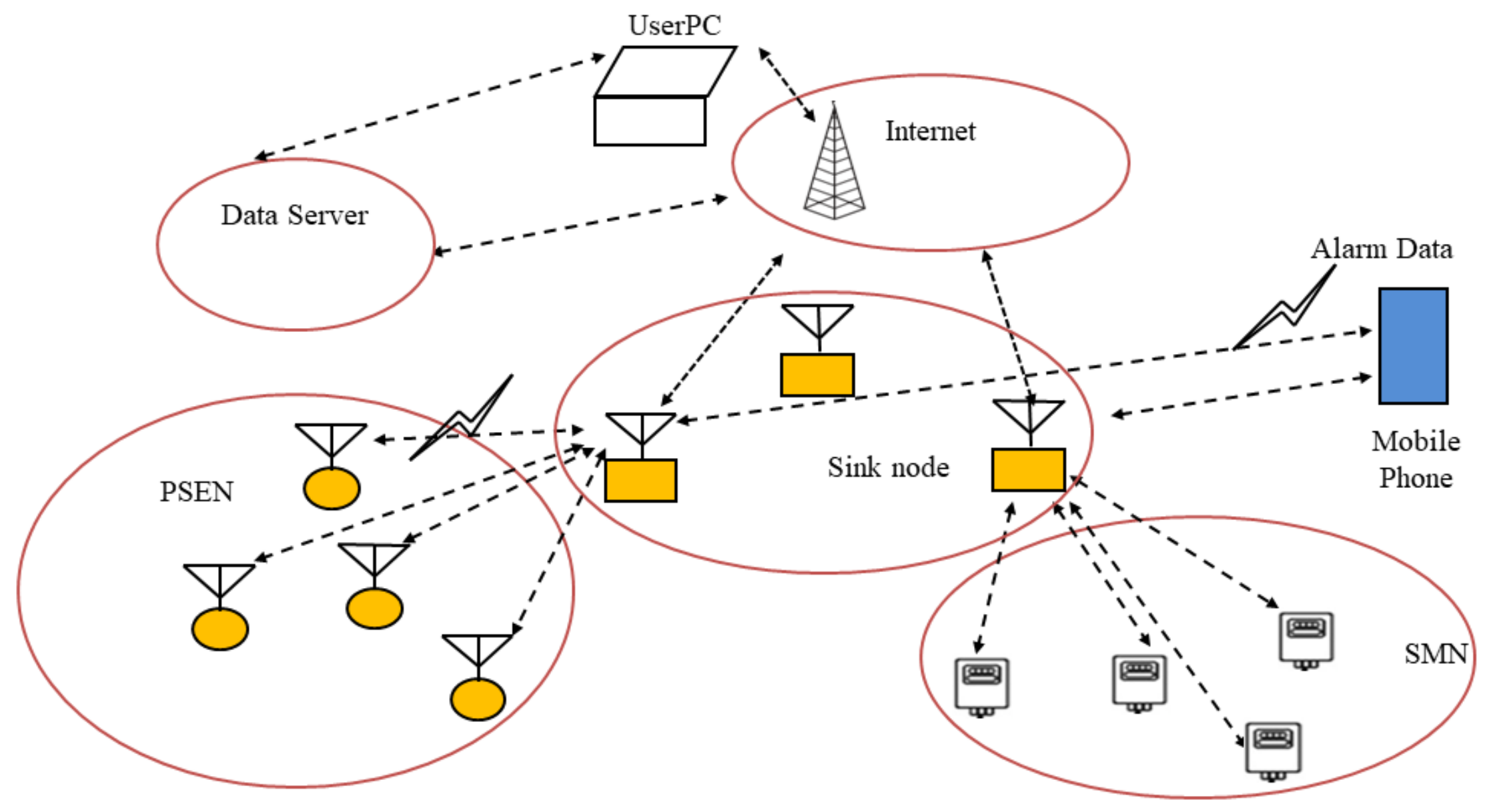
2.1. WSN PSEN-SM System Architecture

As depicted in Figure 1, the WSN smoke and smart meter system has three hierarchy levels and relationships. The first level comprises the PSENs and SMNs, which monitor the smoke, humidity, ambient temperature, and electricity consumption and send the related compressed data to the sink nodes. The PSENs and SMNs receive commands or acknowledgments from the sink nodes. The second level represents the sink nodes (always in an active state), which receive the PSEN and SMN data and send acknowledgments or commands back to them via the radio frequency (RF) module. The sink nodes receive layer commands from the PC via the Internet and simultaneously send related data to the PC via the Internet and alarm signals to the mobile device of an operator. The third level comprises a PC with Internet access and a data server, which receives data from the sink nodes and sends commands back via the Internet. The following section introduces how the PSEN is used. The SMN method is not involved here.

A time-sharing communication protocol is used between the PSENs and the sink node. Each node and module applies a duty-cycling method to reduce charge consumption. Moreover, the sink node of the WSN has high performance, which can reduce the communication time with the PSEN. When all PSENs have a long lifetime, the total lifetime of the WSN can be extended.

2.2. PSEN System Architecture

The PSEN system architecture is illustrated in Figure 2. The system comprises a microcontroller (MCU), an RF module, a power module, and a sensor module. To reduce the charge consumption, each module has a quantity charge model associated with the dominant charge consumer. A component can be regarded as a functional block, and the operational state of various modules is dynamically adapted to the required performance level, which can minimize the power wasted by idle or underutilized components [29]. The PSEN integrates temperature and humidity sensors to detect environmental changes rapidly. For the smoke sensor, we used an ultralow-power photoelectric amplifier with a low supply voltage.

The PSEN is set to a low power state after the interrupt is initialized and opened. When there is an interrupt signal, the MCU wakes up to execute the interrupt events. Since a node battery’s charge is limited, we define three states for the PSEN, namely, the ordinary, warning, and alarm states. The proposed node system can optimize the hardware and software systems, simplify the protocol, and compress signal data.

3. Proposed ELQC Model

Each node in a WSN consists of multiple modules, which can be abstracted as a series, such as 1, 2, …, m, and each module has multiple states, which can also be seen as a sequence 1, 2, …, n. We can encode them as m × n matrices, as expressed in Equation (1). Hence, we can determine the charge consumption of each module in each state.

$$Q_{total}=\left[\begin{array}{c}{Q}_{11} Q_{12} \dots Q_{1j} \dots Q_{1n} \\ Q_{21} Q_{22} \dots Q_{2j} \dots Q_{2n}\\ \cdots \cdots \\ Q_{i1} Q_{i2} \dots Q_{ij} \dots Q_{in}\\ \cdots \cdots \\ Q_{m1} Q_{m2} \dots Q_{mj}\dots Q_{mn} \end{array}\right].$$

(1)

The charge consumption $Q_{ij}$ of the i-th module in the j-th state is the time integral of the current, and its average current $I_{ij}$ at quantum time $T_{ij}$ can be represented by the following:

$$Q_{ij}=\int i_{ij}dt=I_{ij}{T}_{ij},i=1,2\dots m;j=1,2\dots n$$

(2)

The node total charge consumption is the time integral of the current (total sum method), which is the sum of the time integrals of the current for each component at different states and can be represented as follows:

$$Q_{total}={{\displaystyle \sum }}_{i=1}^m{{\displaystyle \sum }}_{j=1}^n{Q}_{ij}={{\displaystyle \sum }}_{i=1}^m{{\displaystyle \sum }}_{j=1}^n\int i_{ij}dt={{\displaystyle \sum }}_{i=1}^m{{\displaystyle \sum }}_{j=1}^n{I}_{ij}{T}_{ij},i=1,2\dots m,j=1,2\dots n$$

(3)

The average current $I_{total-aver.}$ and time $T_{total}$ matrices for the nodes in various states are represented by the following:

$$I_{total-aver.}=\left[\begin{array}{c}{I}_{11} I_{12} \dots I_{1j} \dots I_{1n} \\ I_{21} I_{22} \dots I_{2j} \dots I_{2n}\\ \cdots \cdots \\ I_{i1} I_{i2} \dots I_{ij} \dots I_{in}\\ \cdots \cdots \\ I_{m1} I_{m2} \dots I_{mj}\dots I_{mn} \end{array}\right], T_{total}=\left[\begin{array}{c}{T}_{11} T_{12} \dots T_{1j} \dots T_{1n} \\ T_{21} T_{22} \dots T_{2j} \dots T_{2n}\\ \cdots \cdots \\ T_{i1} T_{i2} \dots T_{ij} \dots T_{in}\\ \cdots \cdots \\ T_{m1} T_{m2}\dots T_{mj}\dots T_{mn} \end{array}\right].$$

(4)

The total charge consumption of the node is the sum of the consumption of each module, and $Q_{Mi}=\left[Q_{i1}{Q}_{i2}\dots Q_{ij}\dots Q_{in}\right]$ denotes the charge consumption of the i-th module including n states. These are abbreviated as follows:

$$Q_{total}={{\displaystyle \sum }}_{i=1}^m{Q}_{Mi},i=1,2\dots m$$

(5)

First, we study the calculations of the i-th module. The charge consumption $Q_{Mi}$ is the sum of the i-th module in the different n states, which is the sum of the corresponding item scores of the two matrices in the i-th row in Equation (4), represented as follows:

$$Q_{Mi}={{\displaystyle \sum }}_{j=1}^n{Q}_{ij}={{\displaystyle \sum }}_{j=1}^n\int i_{ij}dt={{\displaystyle \sum }}_{j=1}^n{I}_{ij}{T}_{ij},i=1,2\dots m,j=1,2\dots n$$

(6)

During the period of the i-th module in all states, the average current and period $I_{Mi} \mathrm{and} T_{Mi}$ for the i-th module of the node is given by the following:

$$I_{Mi}=\frac{Q_{Mi}}{T_{Mi}}=\frac{{{\displaystyle \sum }}_{j=1}^n{I}_{ij}{T}_{ij}}{{{\displaystyle \sum }}_{j=1}^n{T}_{ij}},T_{Mi}={{\displaystyle \sum }}_{j=1}^n{T}_{ij},j=1,2\dots m,j=1,2\dots n,$$

(7)

Similar to real-world node implementations, we divided the states of the i-th module into working, idle listening, and standby states.$\left(I_{wi},T_{wi}\right), (I_{sti}, T_{sti}), \mathrm{and} (I_{li}, T_{li})$ are the currents and times corresponding to the working, standby, and idle listening states, respectively. In general, $I_{li}>I_{sti}$. In the sleep state, the current is almost zero and consumes almost no charge; therefore, it is ignored. These can then be represented as follows:

$$\begin{gathered} I_{Mi}=\frac{ I_{wi}{T}_{wi}+I_{sti} T_{sti}+I_{li}{T}_{li}}{T_{wi}+T_{sti}+T_{li}}=I_{wi}-\left(I_{wi}-I_{li}\right)R_{li}-\left(I_{wi}-I_{sti}\right)R_{sti},i=1, 2\dots m, \\ {R}_{sti}=T_{sti}/T_{Mi}, R_{li}=T_{li}/T_{Mi}=1-(T_{sti}+T_{wi})/T_{Mi},T_{Mi}=T_{wi}+T_{sti}+T_{li}, i=1,2\dots m, \end{gathered}$$

(8)

where $R_{sti} and R_{li}$ denote the standby and idle listening time duty cycle of the i-th module.

If $T_{wi} and I_{wi}$ are fixed, $R_{sti}$ ($1\ge R_{sti}\ge 0$) and $R_{li}$ ($1\ge R_{li}\ge 0$) increase as the standby time $T_{sti}$ and idle listening $T_{li}$ increase. When the other parameters remain unchanged and the standby time is known, then the idle listening duration can be obtained, and vice versa. When $R_{sti}$ and $R_{sli}$ increase, the average current and the charge consumption of the i-th module decrease. The average current and period of the module are represented by the following:

$$I_M=\left[\begin{array}{c}{I}_{M1}\\ I_{M2}\\ \cdots \\ I_{Mi}\\ \cdots \\ I_{Mm}\end{array}\right], T_M=\left[\begin{array}{c}{T}_{M1}\\ T_{M2}\\ \cdots \\ T_{Mi}\\ \cdots \\ T_{Mm}\end{array}\right].$$

(9)

The node’s total average current can be obtained as follows:

$$I_{node-aver}={{\displaystyle \sum }}_{i=1}^m{I}_{Mi},i=1,2\dots m.$$

(10)

The total node charge consumption during the battery’s lifetime is equal to the available battery charge. The quantity of charge Q_battery, availability rate η of the battery, and self-discharge rate R_{self-dischage} can be obtained from the datasheets of the battery. We can then obtain the battery life $T_{batt.life}$ of the WSN node as follows:

$$I_{node-aver.}{T}_{batt.life}=Q_{battery}\eta {\left(1-R_{self-discharge}\right)}^{T_{batt.life}}.$$

(11)

For η of 0.72 and R_{self-discharge} of 3%, the lifetime graph from 0 to 20 years and charge consumption from 950 to 2800 mAh are illustrated in Figure 3. It can be seen that as the current I decreases, the lifetime t of the node increases, as the yellow color in the figure deepens. As the battery capacity Q increases, the allowable current for node with the same lifespan increases, and the light yellow parts in the figure become more numerous.

4. Proposed QL-ELQC Method

To minimize the average current and to extend the node’s life, the designed communication distance is greater than the actual distance, so all nodes can communicate directly with the sink nodes. If other parameters are not changed, when implementing multi-hops between adjacent nodes to the sink node, one data transmission exchanges twice the receiving and transmitting data with the upper and next nodes, but when the node communicates directly with the sink node, it need only exchange once, which can eliminate the charge consumption according to the ELQC model (8).

In special circumstances, some nodes require multi-hops to communicate with the sink node. Since a routing table is used for data transfer, Q-table is used for the next idle listening duration and standby time of a node in WSN. Therefore, this can minimize the time for changing the radio state to RX. The QL-ELQC scheduling method adaptively adjusts the idle listening duration and standby times of the nodes according to the alarm level, which reduces the delay and energy consumption required for data transmission. Here, the QL-ELQC will mainly focus on standby time.

4.1. Proposed QL-ELQC Block Diagram

QL is based on iterative offline operations that predict the next optimal step based on obtained experience. To alert the node in time and to extend its lifetime, we used a QL-ELQC method for duty cycle optimization to determine its operating and propagation strategy in a dynamic environment.

For the proposed QL-ELQC method, the atmospheric sensor data are defined as “state”, while the standby time in the entire period is regarded as an “action”. The level of alarm and the reduction in the average current are the “reward”. In this paper, each node is regarded as an agent that interacts with the environment, calculates the reward, updates the Q-value, self-learns, and selects the optimal state and action, as depicted in Figure 4. Then, the optimal transition between states can send alarm data in time and reduce the quantity of charge consumed to extend the lifetime of the node.

Because the state of the environment is significantly large, the state space is also large. Concurrently, the different duty cycles of standby time in the entire period are considered environmental actions. This renders the typical implementation of QL infeasible. To address this problem, the state classification method adopted in this paper aims to limit the acceptable computational overhead and to reduce the energy and time consumption caused by excessive computational complexity. One of its distinctive features compared with other MAC protocols is that the standby time is modified based on the relationship between the atmospheric sensor data and the threshold. The data compression method can be used when the data are in the same state. Simultaneously, carrier detections exist for “listening before transmitting” protocols and transmissions are repeated if the data are not received. This ensures fast point-to-point communication during alarm states.

4.2. Proposed QL-ELQC Model

4.2.1. QL-ELQC of Standby Time Optimization

Owing to the complexity of atmospheric data in WSNs, the duty cycle must be dynamically altered based on the variable sensor data. The node determines the transmission frequency based on state vector S = (s₁, s₂,…, s_N) and sends the results to the RF module. In this paper, a model with three states and one optimal action was created using a self-learning process and interaction with the atmosphere to satisfy the rapid alarm and early warning requirements of the system. This overcomes the problem caused by major atmospheric conditions and action spaces. Based on the relationship between the monitored data values V and thresholds $V_{th}$, which are set in many experiments, the environmental states are divided into three categories, alarm, warning, and normal states, which can be expressed as follows:

$$S=\left\{\begin{array}{c}{s}_1,V\ge V_{th}, continuous 3 times,in alarm state\\ s_2,V\ge V_{th}, 1-2 times, in warning state \\ s_3,V\le V_{th}, in normal state\end{array}\right..$$

(12)

If the measurement data are larger than the threshold by one time, the node enters the warning state and the sensors immediately increase the monitoring frequency to continuously determine whether it has exceeded the threshold to lessen the error alarm. Subsequently, if one of the data points is still larger than the related threshold, the node system is in an alarm state. The node system then sends the data continuously until the alarm state is cleared, and the sink node system (always active) sends the alarm data to the user PC and the mobile phone of the worker on duty. It continuously reduces the latency through Q-learning training in the alarm state. If the measured data do not exceed the threshold, the node system is in the normal state and the data are processed using the QL-ELQC method to optimize the duty cycle of the node.

In general, the data monitored by sensors do not change significantly in a short period or fluctuate within an allowed range within a certain period. As opposed to continuous monitoring, this can considerably reduce charge consumption. Meanwhile, data aggregation substantially reduces energy consumption compared with transmitting all raw data to the sink node and can reduce traffic and improve the sensing quality for this type of smoke alarm system. The sensors and RF module duty cycles were then optimized using the QL-ELQC method to reduce the charge consumption, considering parameters such as communication distance, operating frequency band, voltage, and current. Therefore, the PSEN with the QL-ELQC quantity charge function to predict the next duration can trigger the alarm in time and can minimize charge consumption.

This policy is crucial for handling the priority relationship between alarms in time and reducing charge consumption. The shorter the standby time, the faster the node system reacts to an alarm state. However, the greater the standby time, the smaller the charge consumption for the node system. The maximum standby time does not exceed the sensitivity requirements of the system. Concurrently, the standby times of the sensor and RF module are not necessarily zero because each module has a minimum time interval. Moreover, in the alarm state, real-time monitoring and communication are superior to the quantity of charge consumed by the smoke alarm system. In an ordinary state, data compression and the duty-cycling algorithm should be prioritized to reduce charge consumption. Based on the sensor data state and policy, QL-ELQC selects an optimal action from the action set A = [T_st1, T_st2, T_st3, T_st4]. The duty cycle of standby time R_st can then be calculated using $R_{sti}=T_{sti}/T_{Mi},$ i = 1, 2,…m:

$$R_{st}=\left[R_{st.al.}, R_{st.war.1},R_{st.war.2},R_{st.nor.}\right],$$

(13)

where $R_{st.al.}, R_{st.war.1},R_{st.war.2}, \mathrm{and} R_{st.nor.}$ are the duty cycles for the standby time of the RF module and sensor module during the alarm, warning 1–2 times, and normal action states, respectively.

In this model, reductions in the node’s average current and the times that the sensor data continuously exceed the threshold are used as reward values to guide the next steps. The more the average current is reduced, the greater the reward in the normal state. The greater the number of times that the data exceed the threshold, the greater the reward value for the alarm level and the smaller the standby time. Using linear regression and function approximation [26], the reward at time t, R_t, can be determined as follows:

$$R_t=\delta I_t+\left(1-\delta \right)l_t+\varnothing ,$$

(14)

where I_t denotes the average current and l_t indicates the level of alarm of the node at time t and the initialization of t = 0. Furthermore, $\delta$ symbolizes the weight of I_t. The reward computed by both the average current and alarm levels ensures an alarm in time and prolongs the lifetime of the node.

The Q function for a node with standby time T_st is represented as $Q_t\left(s_t,R_{st}\right)$, which represents the real value at time t. It is updated based on a dynamic programming concept. If the objective value function $Q_{target}$ at time t is $Q_{target}=R_t+\beta {\max }_{a\in A}{Q}_t\left(s_{t+1},R_{st+1} \right)$, then $\beta$ indicates the discount factor of the node. If A represents a set of actions, ${\mathrm{Max}}_{a\in A}{Q}_t\left(s_{t+1},R_{st+1} \right)$ indicates the largest Q function in the corresponding state s_t+1 at standby time T_st+1. The learning rate $\alpha$ is set as the step size for each update to reduce the difference between the two values; the specific update formula is as follows:

$$Q_{t+1}\left(s_t,T_{st}\right)=Q_t\left(s_t,T_{st}\right)+\alpha [R_t+\beta {\max }_{a\in A}{Q}_t\left(s_{t+1},T_{st+1} \right)-Q_t\left(s_t,T_{st}\right)].$$

(15)

The node adopts the $\epsilon$—greedy strategy to optimize its standby time, rather than directly selecting the maximum Q value as the setting. When Q-table converges, selecting action $a$ in any state $s$ to maximize $Q\left(s,a\right)$ can yield the optimal control strategy $a^{*}={ \mathrm{argmax}}_{a\in A}Q\left(s,a\right)$. An optimization control scheme based on Q-learning is presented in the algorithm.

The values of parameters $\alpha , \beta , \mathrm{and} \epsilon$ are crucial for the algorithm to work properly. If $\alpha$ is too small, the convergence speed of the algorithm will slow down; if $\alpha$ is too high, it may prevent the algorithm from converging or it may experience oscillations. These parameter values were selected by initialization, dynamic adjustment, and experimental verification, based on the Algorithm 1’s performance and convergence.

Algorithm 1: Standby time optimization control scheme based on QL-ELQC

1: Initialization $\epsilon =0.1, \alpha =0.1, \beta =0.9, t=0, Q\left(s,R_{st}\right)=0$; 2: Observation sensor data and status st Equation (12); 3: Select standby time optimization action value control scheme based on the $\epsilon$—greedy strategy Tst; 4: Set the standby time according to policy and calculate Rst Equation (13); 5: Obtain the instant reward value Equation (14); 6: Update $Q_t\left(s_t,T_{st}\right), Q_t\left(s_{t+1},T_{st+1}\right)$. according to Equation (15); 7: Determine whether the learning process has ended. If not, set t = t + 1 and return to step 2, else end the learning procedure.

4.2.2. Simulation Results

To verify the algorithm, ten nodes were deployed at distances of 30 m using a tree topology. The transmission distance for each node was set to 55 m. One node is a sink node (always active). The other node sensor modules detect the environment and generate data at intervals of 10 s in the normal state and 1 s in the alarm state. As analyzed above, the three different atmospheric states were classified based on the relationship between the data, threshold, and state set S = [s₁, s₂, s₃]. The different standby time choices of the RF module and sensor module were considered environmental actions. Action set A = [a₁, a₂, a₃, a₄], initialization at t = 0, the node learning rate $\alpha =0.1,$ discount factor $\beta =0.9$, $\varnothing =4, \delta =2,$ and $\epsilon =0.1$ were set. The transmitting, receiving, and standby currents of the RF module were $I_{w.tr}=16 \mathrm{mA},$ $I_{w.rx}=12.5 \mathrm{mA},$ and $I_{st}=0.68 \mathsf{\mu }\mathrm{A}$. Carrier detection exists for “listen before transmit” protocols, and each node sends data based on the allocated time slot to reduce collisions.

As shown in Figure 5, using the two methods, the PSEN’s lifetime was compared in the alarm and normal states. In the alarm state, the PSEN’s lifetime using the two methods is identical. In the normal state, the PSEN’s lifetime under QL-ELQC is longer than that for the QL-Load [26]. This indicates that the QL-ELQC scheme is suitable for the duty cycle of alarm nodes in response to dynamic environmental changes in the WSN. QL-ELQC makes self-adaptive decisions based on the classification of states, actions, and function approximations in a dynamic environment and prolongs the lifetime of the node and the WSN.

This study used the data compression method for the case when the sensor data were in the same state. End-to-end latency in packet transmission is occasionally caused by re-transmissions. Due to the carrier detection measures for “listening before transmitting” protocols and the alarm channel, the delay is generally less than 1 s, which is much smaller than that of other QL schemes.

5. Experimentation

According to the ELQC model, when the PSEN is in a different state, the charge consumption is different. For experimental convenience and to verify that the QL-ELQC prolongs the lifetimes of PSENs, we divided the mode of the i-th module into two categories, namely, working mode $I_{wi},T_{wi}$ and standby mode $I_{sti}, T_{sti}$. Since the current in the sleep state is almost zero, it was ignored. The operating voltage (VCC) was fixed, and the power consumption was calculated from the current in the module connection path. Thus, the low dropout regulator (LDO) fixed the VCC to measure the current of each module circuit using an oscilloscope (RIGOL DS1074). In the figures, the relation between the I_w values in the tables and the voltage values registered by the oscilloscope is 10 mV/mA and 1 mV/μA.

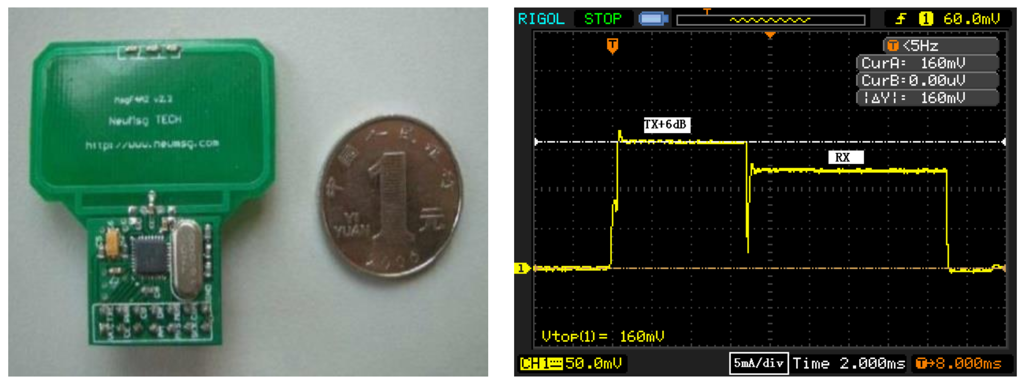
5.1. RF Module

The RF module is integrated via an nRF905 Nordic chip, as depicted in Figure 6; the specifications and measured currents of the RF module are listed in

Table 1. RF module parameters of the PSEN in different states.

State		Iw	Time			Dist.(m)
			TW (ms)	TNor-st. (s)	Tal.st (ms)
RX		12.5 mA	10	86,400	220
TX	+6 dBm	16.0 mA	7	86,400	220	40–55
Standby		0.68 μA	All time		0	0

. T_Nor.lt. indicates the maximum time of the RF module in standby mode under normal environmental conditions, and T_al.lt indicates the minimum value of the RF module in the alarm state. This means that the range of standby time $T_{RF.st}$ for the RF module is $0.22\le T_{RF.st}\le \mathrm{86,400} \mathrm{s}.$ In this experiment, the TX current was 16 mA, and the transmission time was T_tx = 7 ms, while the RX current was 12.5 mA, and the receiving time was T_rx = 10 ms. Thus, the working time and average current of the RF module were approximately T_tx-rx = 17 ms and I_tx-rx = 13,941 μA, respectively.

5.2. Sensor Module

Here, we only list the experimental results for the smoke sensors. The varying current and operating times of the A5303 smoke sensor at different stages were measured in several experiments, as shown in Figure 7.

Table 2. Smoke sensor experimental data for different states (power: 3.3 V).

State		Iw (μA)	Time	Iw.aver. (μA)
			TW (ms)
Smoke sensor during one period	Start	300	10	33
	signal MAX.	500	0.2
	Attenua. meas.	50	100
		25	100
		20	100
		10	100
Standby		2.6	All time	2.6

lists the varying currents to the smoke sensors. With a large value at the starting point, the signals promptly increased to the maximum value and then gradually slowed down. The average current was 33 μA, which can be calculated using Equation (7), and the operating time was approximately 410 ms when it detected the environment once. With values lower than the threshold, the operational interval is 10 s, and the sensor is in standby mode. When the value exceeds the threshold, the sensor measures the environment three times repeatedly at 1 s intervals. This means that the standby time $T_{sen.st}$ range for the sensor is $1\le T_{sen.st}\le 10 \mathrm{s}.$

5.3. MCU

Microcontrollers are widely used in terminal devices. Therefore, they are listed separately and discussed herein. The PSEN system used a low-power-consumption MCUMSP430 from Texas Instruments. The software uses the interrupts of the MCU to awaken the standby state to execute the QL-ELQC period monitoring, to compress data, to set the alarm, to transmit data, and to receive commands or acknowledgments from the sink node. The clock system is specifically designed for battery-powered applications.

Table 3. MCU experimental data of the PSEN in different states (power: 3.3 V).

State	Iw.aver	Tw
Low battery detect	420 μA	120 ms
Environment detect	420 μA	120 ms
Environ. detect & RF	500 μA	250 ms
Standby	1.96 μA	10 s

presents the experimental results for the MSP430 when the PSEN was in different states. Environmental monitoring included monitoring the temperature, humidity, and smoke.

5.4. Power Management

In this study, we used the analog-to-digital converter (ADC) feature of an MCU MSP430F149 to detect the battery voltage periodically (10 s in the normal state and 1 s in the alarm state). The reference voltage of the ADC was 2.5 V, and resistors R1 and R2 were used to distribute the battery voltage. The circuit of the low-battery detector is shown on the left-hand side of Figure 8.

The new battery’s voltage is slightly higher than the nominal voltage, and the AD VBAT voltage is greater than the break-over voltage for the clamp diode of the AD VBAT input buffer, which is the circuit in the MCU. In the experiment, when the AD STROBE was set with a high resistance input, the current in decades of μA could be detected through R1. To solve this problem, a new low-battery circuit was designed, as shown in Figure 9.

When the MCU does not detect the battery voltage, AD_STROBE is low and Q3 is off. Simultaneously, the grid voltage of Q4 becomes high and Q4 is off. When Q3 and Q4 are in the off state, AD_VBAT is reduced by R2. Thus, the detection circuit does not consume charge. When the MCU detects the battery voltage, AD_STROBE is high. In this case, Q3 is turned on, which pulls down the grid voltage of Q4, turning Q4 on. In this instance, R1 and R2 distribute the battery voltage, and the MCU detects the voltage of AD_VBAT to obtain the battery voltage.

Table 4. Low-voltage detector experimental data of the PSEN (power: 3.3 V).

Compo.	Stage	Iw (μA)	TW (ms)	Iw.aver. (μA)
Low voltage	IR	1980	12	0.0083
	AD	900	2
	MCU	420	10

lists the low-voltage detector experimental current and operating time of the PSEN. The average current is 0.0083 μA, which can be calculated using Equation (7).

6. PSEN System Measurements and Discussion

Table 5. Experimental data for each module in the normal or alarm state (VCC = 3.3 V).

Module	Iw (μA)	Ist (μA)	Tw (s)	Tnorm-st/lt (s)	Tal.-st (s)	Itotal-ave. (μA)	Ial.ave. (μA)
LDO	11	1.54	0.200	86,400	1	3.14	5.06
	2.5		0.721	10	1
Low-vol.	2488	0	0.012	3600	1	0.0083	29.50
MCU	420	2	0.120	10	1	6.47	46.79
Smoke	33	2.6	0.410	10	1	3.79	11.44
SHT10	386	0.1	0.103	10	1	4.08	36.14
RF-module	16,000	0.68	0.200	86,400	1	0.717	2667.23
Total	6.8					18.65	2796.16

lists the experimental average current for each module and the total average current of the PSEN system. The actual communication time T_tx-rx of the RF module in Table 1 was 17 ms, and the average current of I_tx-rx is 13,941 μA. Note that the redundant RF module’s operational time (200 ms) and the current (16,000 μA) were calculated for the average current I_total-ave. and I_al.ave., considering the collision and retransmitting. The LDO current has three components, among which 1.54 μA was the standby current, 2.5 μA was the PSEN’s current for monitoring the environment, and 11 μA was the PSEN’s current for communicating with the sink node. Based on these currents, as well as T_w and T_st, the average LDO current under normal and alarm states was determined as 3.14 μA and 5.06 μA using Equation (7), respectively.

From the module measurements, we obtained the average current for different components using Equation (7), and then, the total average standby current of all components was calculated to be 6.92 μA, which is close to the PSEN’s total system standby current of 6.8 μA obtained from the experiment. As shown in

Table 6. Theoretical and experimental data of the PSEN standby current.

Standby Parameters of the Node System	I (μA)
Experimental	6.8
Theoretical calculation	6.92
Error (%)	1.73

, the error between the measurements and calculation with ELQC was 1.73%, which verifies the accuracy of the ELQC model.

Meanwhile, the PSEN’s total normal average current was 18.65 μA, and the total average current was 2.79 mA in the alarm state. As shown in Figure 10, the standby time (86,400 s) set by the QL-ELQC in the normal state was much longer than that (1 s) in the alarm state, and the current in the normal state was approximately 1/150 times lower than that in the alarm state. The advantage is not reflected enough within 10 s, and the longer the standby time, the more obvious the advantage. When power equipment operates normally, the probability of smoke occurrence remains extremely low; therefore, the QL-ELQC method used in the normal state significantly extends the total lifespan of the PSEN.

The simulation lifetime of the PSEN is 9.2 years for E91 in Figure 5, which is similar to a theoretical lifetime of 9.29 years but so long that we cannot test it for approximately 10 years, based on a practical system current of 18.65 μA. Using Equation (7), we can vary the current and change the lifetime of the PSEN to test the low-quantity charge design method; namely, we can select a small Q_battery and shorten the lifetime for the test. Here, we used three E92 (not ordinary E91) small batteries, which have an approximately 950-mAh charge ranging from 1.6 to 1.2 V. The relevant data for the tested system are presented in

Table 7. Measurement and theoretical lifetime of the PSEN with increasing transmission times.

Battery Type	E92
Quantity charge from 1.6 to 1.2 V	950 mAh
Tested practical lifetime (h)	181
Calculation lifetime (h)	173.35
Error (%)	4

. By increasing the communication times of the PSEN to every half second with sensors continuously monitoring the environment, the current of the PSEN can be increased. Thus, the current of the tested system is 5.48 mA (not 18.65 μA) to shorten the lifetime of the test, and the calculation lifetime is 173.35 h. When the voltage decreased to 1.2 V, the practical lifetime of our tested system was 181 h, and the error was 7.64 h, which is approximately 4%. As our proposed method considers redundancy, the tested system ran slightly longer than the calculated lifetime. Through practical experiments and algorithms, we tested the lifetime of a photoelectric smoke node and verified that our method, which is based on the charge quantity, is reasonable. Our proposed approach is general and can be applied to alarm scenarios where the node requires long-term operation.

7. Conclusions

In this paper, a Q-learning and efficient low-quantity charge (QL-ELQC) method is presented for the smoke alarm unit of a power system to reduce the average current and to improve the lifetime of the nodes of wireless sensor networks (WSNs). Analytical functions were derived to describe the behavior of the parameters versus those with which they were compared. The Q-learning-based ELQC method was applied to self-adjust the standby time of the modules to optimize the duty cycle of the sensor and RF modules to prolong the lifetime of the node system. This could effectively overcome the continuous state–action space limitations of Q-learning using the state classification method. Methods were used to extend the lifetime of PSENs in WSNs by reducing the average current in each module and every state, respectively. The simulation results reveal that the proposed scheme significantly improves the lifetime compared with the existing QL-Load scheme. Furthermore, the experimental results are consistent with the theoretical results. The model appears to be accurate for nodes in WSNs. The experimental results show that the proposed QL-ELQC method extends the lifetime of the PSEN, which is capable of long-term operation. We concluded that the QL-ELQC method proposed in this paper can be used for reference to prolong the lifetime of the node in alarm scenarios where batteries cannot be replaced or recharged under harsh environmental conditions.

References

- Bhuiyan, M.N.; Rahman, M.M.; Billah, M.M.; Saha, D. Internet of Things (IoT): A review of its enabling technologies in healthcare applications, standards protocols, security, and market opportunities. IEEE Internet Things J. 2021, 8, 10474–10498. [Google Scholar] [CrossRef]
- Ghayvat, H.; Mukhopadhyay, S.; Gui, X.; Suryadevara, N. WSN- and IOT-based smart homes and their extension to smart buildings. Sensors 2015, 15, 10350–10379. [Google Scholar] [CrossRef] [PubMed]
- Lazarescu, M.T. Design of a WSN platform for long-term environmental monitoring for IoT applications. IEEE J. Emerg. Sel. Topics Circuits Syst. 2013, 3, 45–54. [Google Scholar] [CrossRef]
- Zhang, Y.; Wang, W.; Xie, H.; Du, S.; Ma, M.; Zeng, Q. Wireless multi-node uRLLc B5G/6G networks for critical services in electrical power systems. Energies 2022, 15, 9437. [Google Scholar] [CrossRef]
- Tarighi, R.; Farajzadeh, K.; Hematkhah, H. Prolong network lifetime and improve efficiency in WSNUAV systems using new clustering parameters and CSMA modification. Int. J. Commun. Syst. 2020, 33, e4324. [Google Scholar] [CrossRef]
- Hatime, H.; Namuduri, K.; Watkins, J.M. OCTOPUS: An on-demand communication topology updating strategy for mobile sensor networks. IEEE Sens. J. 2011, 11, 1004–1012. [Google Scholar] [CrossRef]
- Yu, C.M.; Ku, M.L.; Wang, L.C. Balanced Routing Algorithm with Transmission Range Adjustment for Network Lifetime Improvement in WSNs. In Proceedings of the IEEE 13th Annual Ubiquitous Computing, Electronics and Mobile Communication Conference (UEMCON), New York, NY, USA, 26–29 October 2022; pp. 308–312. [Google Scholar]
- Wang, W.S.; Huang, H.Y.; Chen, S.C.; Ho, K.C.; Lin, C.Y.; Chou, T.C.; Hu, C.H.; Wang, W.F.; Wu, C.F.; Luo, C.H. Real-time telemetry system for amperometric and potentiometric electrochemical sensors. Sensors 2011, 11, 8593–8610. [Google Scholar] [CrossRef]
- Koo, B.; Shon, T. Implementation of a WSN-based structural health monitoring architecture using 3D and AR mode. IEICE Trans. Commun. 2010, E93.B, 2963–2966. [Google Scholar] [CrossRef]
- Mahdi Elsiddig Haroun, F.; Mohamad Deros, S.N.; Ahmed Alkahtani, A.; Md Din, N. Towards self-powered WSN: The design of ultra-low-power wireless sensor transmission unit based on indoor solar energy harvester. Electronics 2022, 11, 2077. [Google Scholar] [CrossRef]
- Hassan, A.A.; Shah, W.M.; Habeb, A.-H.H.; Othman, M.F.I.; Al-Mhiqani, M.N. An improved energy-efficient clustering protocol to prolong the lifetime of the WSN-based IoT. IEEE Access 2020, 8, 200500–200517. [Google Scholar] [CrossRef]
- Li, N.; Xiao, M.; Rasmussen, L.K.; Hu, X.; Leung, V.C.M. On resource allocation of cooperative multiple access strategy in energy-efficient industrial Internet of things. IEEE Trans. Ind. Inf. 2021, 17, 1069–1078. [Google Scholar] [CrossRef]
- Panhwar, M.A.; Liang, D.Z.; Memon, K.A.; Khuhro, S.A.; Abbasi, M.A.K.; Noor-ul-Ain, Z.A.; Ali, Z. Energy-efficient routing optimization algorithm in WBANs for patient monitoring. J. Ambient Intell. Hum. Comput. 2021, 12, 8069–8081. [Google Scholar] [CrossRef]
- Xie, J.Z.; Zhang, B.J.; Zhang, C.P. A novel relay node placement and energy efficient routing method for heterogeneous wireless sensor networks. IEEE Access 2020, 8, 202439–202444. [Google Scholar] [CrossRef]
- Liu, S.; Fan, K.W.; Sinha, P. CMAC: An energy-efficient MAC layer protocol using convergent packet forwarding for wireless sensor networks. ACM Trans. Sens. Netw. (TOSN) 2009, 5, 29. [Google Scholar] [CrossRef]
- Khoramnejad, F.; Joda, R.; Sediq, A.B.; Abou-Zeid, H.; Atawia, R.; Boudreau, G.; Erol-Kantarci, M. Delay-aware and energy-efficient carrier aggregation in 5G using double Deep Q-networks. IEEE Trans. Commun. 2022, 70, 6615–6629. [Google Scholar] [CrossRef]
- Wu, Z.; Pan, P.; Liu, J.; Shi, B.; Yan, M.; Zhang, H. Environmental perception Q-learning to prolong the lifetime of poultry farm monitoring networks. Electronics 2021, 10, 3024. [Google Scholar] [CrossRef]
- Tarasia, N.; Swain, A.R.; Roy, S.; Kar, U.N. Improved localized sleep scheduling techniques to prolong WSN lifetime. Scalable Comput. Pract. Exp. 2021, 22, 81–92. [Google Scholar] [CrossRef]
- Yao, Y.-D.; Wang, C.; Li, X.; Zeng, Z.; Zhao, B.; Su, Z.; Li, H. Multihop clustering routing protocol based on improved coronavirus herd immunity optimizer and Q-learning in WSNs. IEEE Sens. J. 2023, 23, 1645–1659. [Google Scholar] [CrossRef]
- Tao, J.; Zhang, R.; Qiao, Z.; Ma, L. Q-Learning-based fuzzy energy management for fuel cell/supercapacitor HEV. Trans. Inst. Meas. Control 2022, 44, 1939–1949. [Google Scholar] [CrossRef]
- Hsu, R.C.; Lin, T.-H.; Su, P.-C. Dynamic energy management for perpetual operation of energy harvesting wireless sensor node using fuzzy Q-learning. Energies 2022, 15, 3117. [Google Scholar] [CrossRef]
- Karunanayake, P.N.; Könsgen, A.; Weerawardane, T.; Förster, A. Q learning based adaptive protocol parameters for WSNs. J. Commun. Netw. 2023, 25, 76–87. [Google Scholar] [CrossRef]
- Hajizadeh, H.; Nabi, M.; Goossens, K. Decentralized configuration of TSCH-based IoT networks for distinctive QoS: A deep reinforcement learning approach. IEEE Internet Things J. 2023, 10, 16869–16880. [Google Scholar] [CrossRef]
- Al-Jerew, O.; Bassam, N.A.; Alsadoon, A. Reinforcement learning for delay tolerance and energy saving in mobile wireless sensor networks. IEEE Access 2023, 11, 19819–19835. [Google Scholar] [CrossRef]
- Redhu, S.; Hegde, R.M. Cooperative network model for joint mobile sink scheduling and dynamic buffer management using Q-learning. IEEE Trans. Netw. Serv. Manage. 2020, 17, 1853–1864. [Google Scholar] [CrossRef]
- Huang, H.Y.; Kim, K.T.; Youn, H.Y. Determining node duty cycle using Q-learning and linear regression for WSN. Front. Comput. Sci. 2021, 15, 151101. [Google Scholar] [CrossRef]
- Shafiq, M.; Ashraf, H.; Ullah, A.; Tahira, S. Systematic literature review on energy efficient routing schemes in WSN—A survey. Mobile Netw. Appl. 2020, 25, 882–895. [Google Scholar] [CrossRef]
- Kamble, A.A.; Patil, B.M. Systematic analysis and review of path optimization techniques in WSN with mobile sink. Comput. Sci. Rev. 2021, 41, 100412. [Google Scholar] [CrossRef]
- Chen, H.; Qin, Y.; Lin, K.; Luan, Y.; Wang, Z.; Yu, J.; Li, Y. PWEND: Proactive wakeup based energy-efficient neighbor discovery for mobile sensor networks. Ad. Hoc. Netw. 2020, 107, 102247. [Google Scholar] [CrossRef]