
Graph- and Machine-Learning-Based Texture Classification


Abstract
:1. Introduction
- This study employed a modified visibility graph to classify a texture dataset using a graph-based classification method.
- The degree distribution information extracted from the IHVG and INVG was used as the input for a specialized classifier.
- This analysis primarily focused on capturing minor substructures by examining the clustering coefficient with the degree distribution for the IHVG and INVG.
2. Related Work
2.1. Texture Classification Based on Traditional Methods
2.2. Texture Classification Based on CNN

| References | Purpose | Features | Model | Dataset | Accuracy (%) |
|---|---|---|---|---|---|
| [27] | Land use classification from satellite images | Image texture features | Depth feature extraction using customized CNN | PaviaU dataset, Salinas dataset, Indian Pines | CNN ELEM 90 |
| [28] | Texture classification | Feature optimization | CNN optimized through WOA | Kylberg Brodatz OutexTC00012 | 99.71 97.43 97.70 |
| [29] | Texture classification | Fusion of AlexNet and VGG | AlexNet layer VGG net layer | Brodatz KTH-TIPS CUReT | 98.76 100 99.76 |
| [13] | Texture classification | CNN features and Gabor features | CaffeNet | Cifar10 dataset | 79.16 |
| [30] | Texture classification | CNN features | New CNN proposed | Brodatz texture database | Error rate (mean) 17.2 |
| [31] | Classification of different ship types | Multiscale rotation invariance CNN features | New CNN developed based on CaffeNet | BCCT200- RESIZE data | 98.33 |
| [32] | Classify benign and malignant masses | Deep texture features | SVM classifier and ELM | Breast CAD of 400 cases | 80.6 to 91 |
| [12] | Texture classification | CNN features | Pre-trained CNN model | KTH-TIPS CURET-Gray | ResNet 98.75, 97.22 DenseNet 99.35, 98.06 |
2.3. Limitations of Traditional and CNN-Based Texture Classification
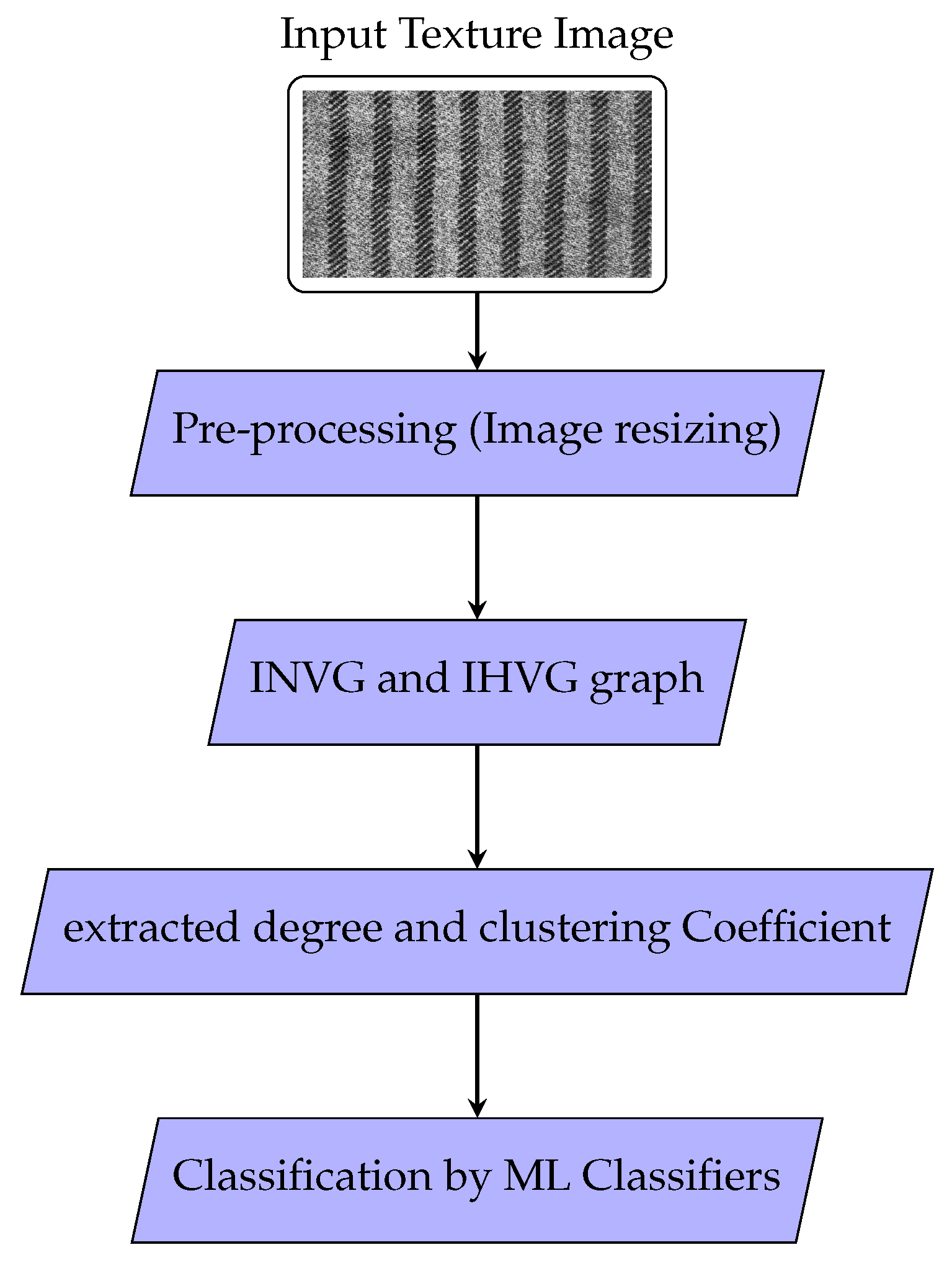
3. Methodology
3.1. Complex Network
3.2. Visibility Graph (VG)
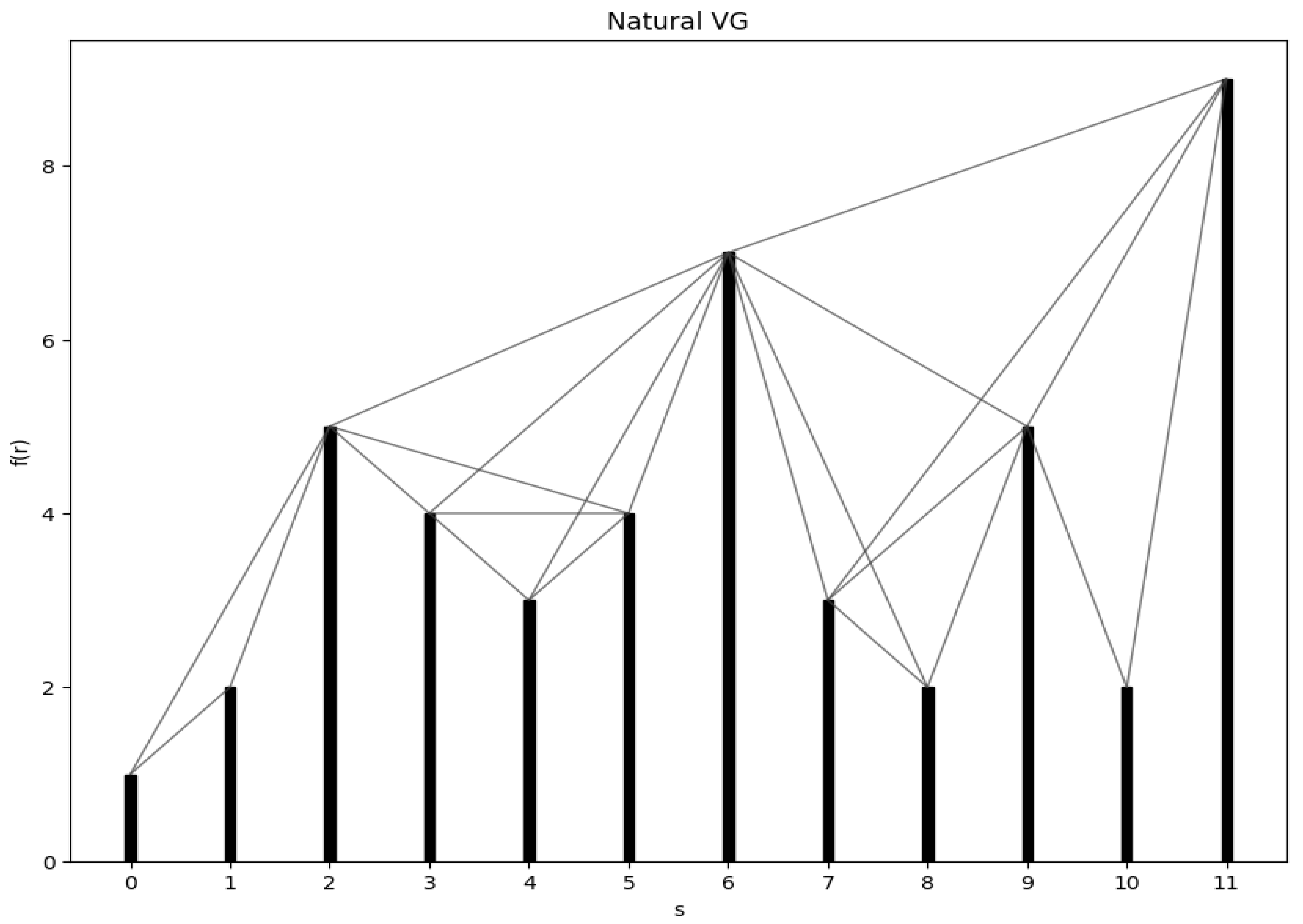
3.2.1. Natural Visibility Graph
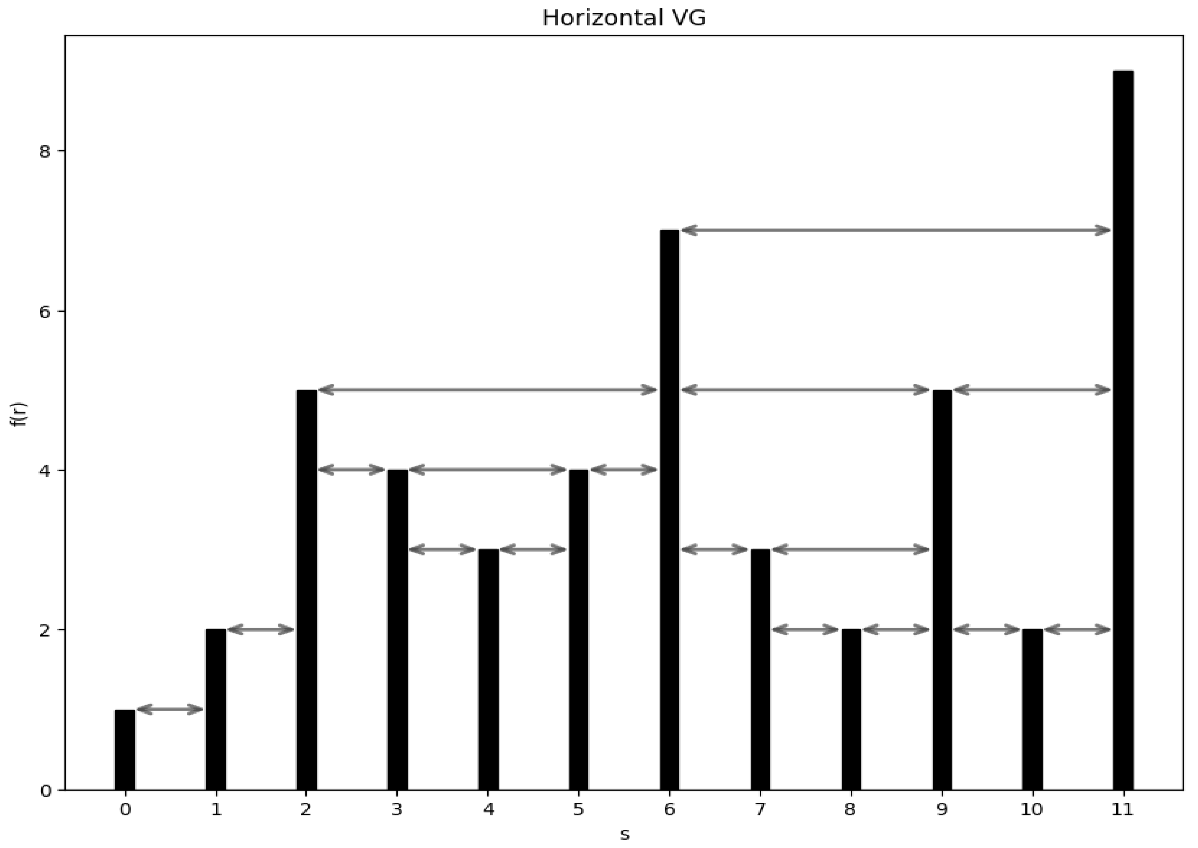
3.2.2. Horizontal Visibility Graph
3.3. Image Visibility Graph
3.3.1. Image Natural Visibility Graph
- OR OR for some integer t and
- the NVG definition algorithm establishes a connection between and . This algorithm is executed on an ordered sequence that comprises and .
3.3.2. Image Horizontal Visibility Graph
- OR OR for some integer t and
- the HVG definition algorithm establishes a connection between and , both of which are included in an ordered sequence.
3.4. Feature Extraction
3.4.1. Degree Distribution
3.4.2. Clustering Coefficient
3.5. Classifiers for Texture Classification
4. Experimental Results and Discussion
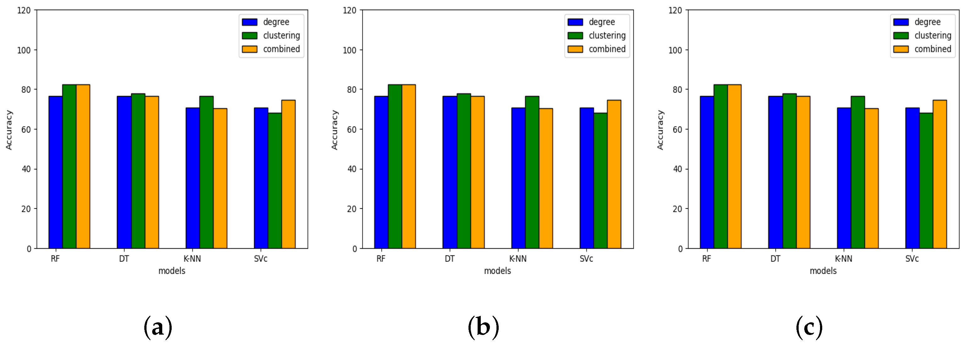
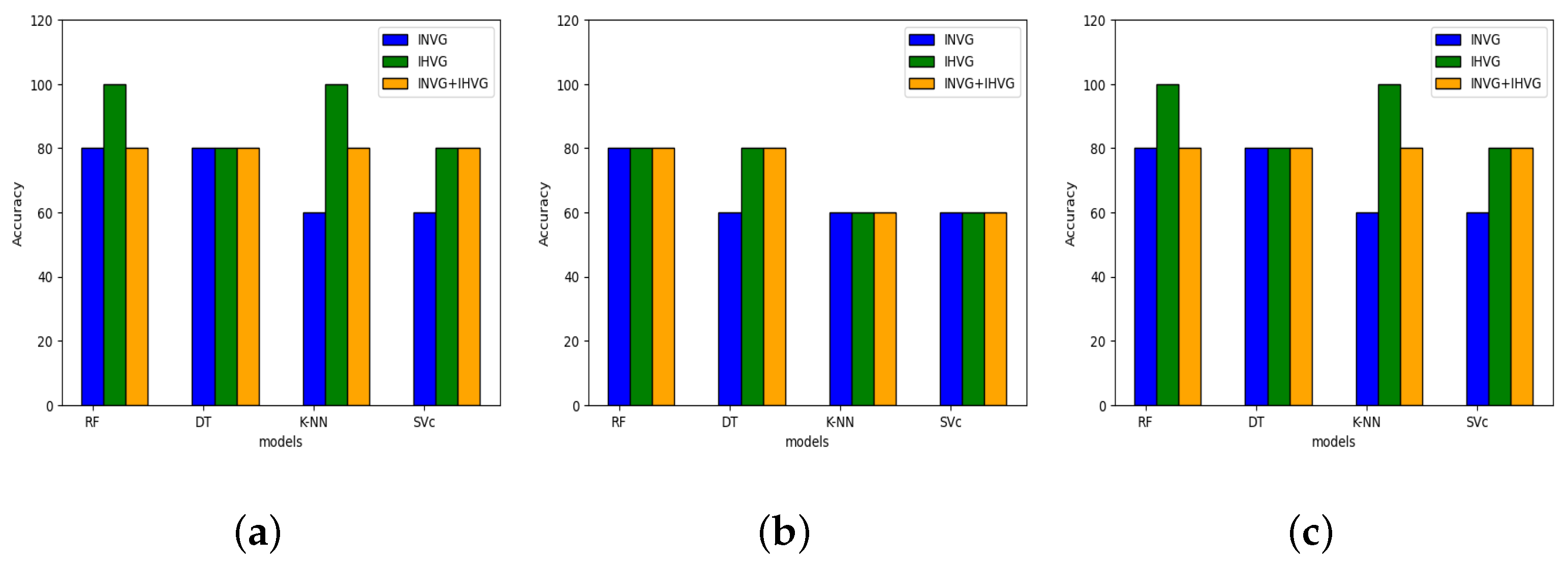
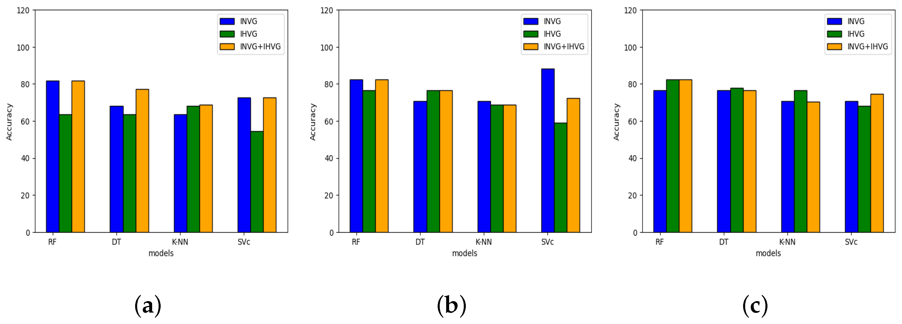
4.1. Classification Results on Brodatz Texture Image Dataset
4.2. Classification Results on Salzburg Texture Image Dataset
4.3. Comparison with Some Existing Methods
5. Conclusions and Future Work
Author Contributions
Funding
Data Availability Statement
Conflicts of Interest
References
- Ataky, S.T.M.; Saqui, D.; de Matos, J.; de Souza Britto Junior, A.; Lameiras Koerich, A. Multiscale Analysis for Improving Texture Classification. Appl. Sci. 2023, 13, 1291. [Google Scholar] [CrossRef]
- Backes, A.R.; Casanova, D.; Bruno, O.M. Texture analysis and classification: A complex network-based approach. Inform. Sci. 2013, 219, 168–180. [Google Scholar] [CrossRef]
- Tuceryan, M.; Jain, A.K. Texture analysis. In Handbook of Pattern Recognition and Computer Vision; World Scientific Publishing Company: Singapore, 1993; pp. 235–276. [Google Scholar]
- Liu, L.; Chen, J.; Fieguth, P.; Zhao, G.; Chellappa, R.; Pietikäinen, M. From BoW to CNN: Two decades of texture representation for texture classification. Int. J. Comput. Vis. 2019, 127, 74–109. [Google Scholar] [CrossRef]
- Iqbal, N.; Mumtaz, R.; Shafi, U.; Zaidi, S.M.H. Gray level co-occurrence matrix (GLCM) texture based crop classification using low altitude remote sensing platforms. PeerJ Comput. Sci. 2021, 7, e536. [Google Scholar] [CrossRef] [PubMed]
- Haralick, R.M.; Shanmugam, K.; Dinstein, I.H. Textural features for image classification. IEEE Trans. Syst. Man Cybernet. 1973, SMC-3, 610–621. [Google Scholar] [CrossRef]
- Arivazhagan, S.; Ganesan, L. Texture classification using wavelet transform. Pattern Recognit. Lett. 2003, 24, 1513–1521. [Google Scholar] [CrossRef]
- Salinas, R.; Gomez, M. A new technique for texture classification using markov random fields. Int. J. Comput. Commun. Control 2006, 1, 41–51. [Google Scholar] [CrossRef]
- Luimstra, G.; Bunte, K. Adaptive Gabor Filters for Interpretable Color Texture Classification. In Proceedings of the 30th European Symposium on Artificial Neural Networks (ESANN), Bruges, Belgium, 5–7 October 2022; pp. 61–66. [Google Scholar]
- Luo, Q.; Su, J.; Yang, C.; Silven, O.; Liu, L. Scale-selective and noise-robust extended local binary pattern for texture classification. Pattern Recognit. 2022, 132, 108901. [Google Scholar] [CrossRef]
- Ataky, S.T.M.; Koerich, A.L. A novel bio-inspired texture descriptor based on biodiversity and taxonomic measures. Pattern Recognit. 2022, 123, 108382. [Google Scholar] [CrossRef]
- Simon, P.; Uma, V. Deep learning based feature extraction for texture classification. Procedia Comput. Sci. 2020, 171, 1680–1687. [Google Scholar] [CrossRef]
- Tianyu, Z.; Zhenjiang, M.; Jianhu, Z. Combining cnn with hand-crafted features for image classification. In Proceedings of the 2018 14th IEEE International Conference on Signal Processing (ICSP), Beijing, China, 12–16 August 2018; pp. 554–557. [Google Scholar]
- Van Hoai, D.P.; Hoang, V.T. Feeding Convolutional Neural Network by hand-crafted features based on Enhanced Neighbor-Center Different Image for color texture classification. In Proceedings of the 2019 International Conference on Multimedia Analysis and Pattern Recognition (MAPR), Ho Chi Minh City, Vietnam, 9–10 May 2019; pp. 1–6. [Google Scholar]
- Pei, L.; Li, Z.; Liu, J. Texture classification based on image (natural and horizontal) visibility graph constructing methods. Chaos Interdisciplin. J. Nonlinear Sci. 2021, 31, 013128. [Google Scholar] [CrossRef]
- Iacovacci, J.; Lacasa, L. Visibility graphs for image processing. IEEE Trans. Pattern Anal. Mach Intell. 2019, 42, 974–987. [Google Scholar] [CrossRef] [PubMed]
- Saini, D.; Kumar, S.; Singh, M.K.; Ali, M. Two view NURBS reconstruction based on GACO model. Complex Intell. Syst. 2021, 7, 2329–2346. [Google Scholar] [CrossRef]
- Kumar, S.; Kumar, S.; Sukavanam, N.; Raman, B. Human visual system and segment-based disparity estimation. AEU-Int. J. Electron. Commun. 2013, 67, 372–381. [Google Scholar] [CrossRef]
- Kumar, S.; Bhatnagar, G.; Raman, B. Security of stereo images during communication and transmission. Adv. Sci. Lett. 2012, 6, 173–179. [Google Scholar] [CrossRef]
- Cavalin, P.; Oliveira, L.S. A review of texture classification methods and databases. In Proceedings of the 2017 30th SIBGRAPI Conference on Graphics, Patterns and Images Tutorials (SIBGRAPI-T), Niteroi, Brazil, 17–18 October 2017; pp. 1–8. [Google Scholar]
- Ojala, T.; Pietikäinen, M. Unsupervised texture segmentation using feature distributions. Pattern Recognit. 1999, 32, 477–486. [Google Scholar] [CrossRef]
- Liao, S.; Law, M.W.; Chung, A.C. Dominant local binary patterns for texture classification. IEEE Trans. Image Process. 2009, 18, 1107–1118. [Google Scholar] [CrossRef]
- Kumar, S.; Kumar, S.; Raman, B. Image disparity estimation based on fractional dual-tree complex wavelet transform: A multi-scale approach. Int. J. Wavelets Multiresolut. Inform. Process. 2013, 11, 1350004. [Google Scholar] [CrossRef]
- Suresh, A.; Shunmuganathan, K.L. Image texture classification using gray level co-occurrence matrix based statistical features. Eur. J. Sci. Res. 2012, 75, 591–597. [Google Scholar]
- Hosny, K.M.; Magdy, T.; Lashin, N.A.; Apostolidis, K.; Papakostas, G.A. Refined Color Texture Classification Using CNN and Local Binary Pattern. Math. Probl. Eng. 2021, 2021, 5567489. [Google Scholar] [CrossRef]
- Lacasa, L.; Iacovacci, J. Visibility graphs of random scalar fields and spatial data. Phys. Rev. E 2017, 96, 012318. [Google Scholar] [CrossRef] [PubMed]
- Huang, F.; Lu, J.; Tao, J.; Li, L.; Tan, X.; Liu, P. Research on optimization methods of ELM classification algorithm for hyperspectral remote sensing images. IEEE Access 2019, 7, 108070–108089. [Google Scholar] [CrossRef]
- Dixit, U.; Mishra, A.; Shukla, A.; Tiwari, R. Texture classification using convolutional neural network optimized with whale optimization algorithm. SN Appl. Sci. 2019, 1, 655. [Google Scholar] [CrossRef]
- Roy, S.K.; Dubey, S.R.; Chanda, B.; Chaudhuri, B.B.; Ghosh, D.K. Texfusionnet: An ensemble of deep cnn feature for texture classification. In Proceedings of the 3rd International Conference on Computer Vision and Image Processing: CVIP 2018; Springer: Berlin/Heidelberg, Germany, 2020; Volume 2, pp. 271–283. [Google Scholar]
- Tivive, F.H.C.; Bouzerdoum, A. Texture classification using convolutional neural networks. In Proceedings of the TENCON 2006—2006 IEEE Region 10 Conference, Hong Kong, China, 14–17 November 2006; pp. 1–4. [Google Scholar]
- Shi, Q.; Li, W.; Zhang, F.; Hu, W.; Sun, X.; Gao, L. Deep CNN with multi-scale rotation invariance features for ship classification. IEEE Access 2018, 6, 38656–38668. [Google Scholar] [CrossRef]
- Wang, Z.; Li, M.; Wang, H.; Jiang, H.; Yao, Y.; Zhang, H.; Xin, J. Breast cancer detection using extreme learning machine based on feature fusion with CNN deep features. IEEE Access 2019, 7, 105146–105158. [Google Scholar] [CrossRef]
- Kumar, S.; Kumar, S.; Raman, B.; Sukavanam, N. Human action recognition in a wide and complex environment. In Proceedings of the Real-Time Image and Video Processing 2011, San Francisco, CA, USA, 24–25 January 2011; Volume 7871, pp. 176–187. [Google Scholar]
- Wen, T.; Chen, H.; Cheong, K.H. Visibility graph for time series prediction and image classification: A review. Nonlinear Dyn. 2022, 110, 2979–2999. [Google Scholar] [CrossRef]
- Zou, Y.; Donner, R.V.; Marwan, N.; Donges, J.F.; Kurths, J. Complex network approaches to nonlinear time series analysis. Phys. Rep. 2019, 787, 1–97. [Google Scholar] [CrossRef]
- Lacasa, L.; Luque, B.; Ballesteros, F.; Luque, J.; Nuno, J.C. From time series to complex networks: The visibility graph. Proc. Nat. Acad. Sci. USA 2008, 105, 4972–4975. [Google Scholar] [CrossRef]
- Luque, B.; Lacasa, L.; Ballesteros, F.; Luque, J. Horizontal visibility graphs: Exact results for random time series. Phys. Rev. E 2009, 80, 046103. [Google Scholar] [CrossRef]
- Luque, B.; Lacasa, L. Canonical horizontal visibility graphs are uniquely determined by their degree sequence. Eur. Phys. J. Spec. Top. 2017, 226, 383–389. [Google Scholar] [CrossRef]
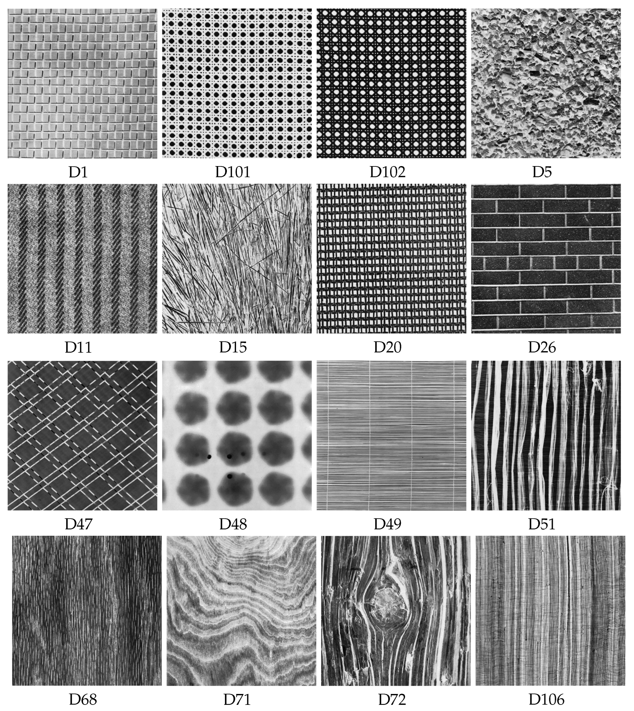
- Abdelmounaime, S.; Dong-Chen, H. New Brodatz-based image databases for grayscale color and multiband texture analysis. Int. Sch. Res. Not. 2013, 2013, 876386. [Google Scholar] [CrossRef]
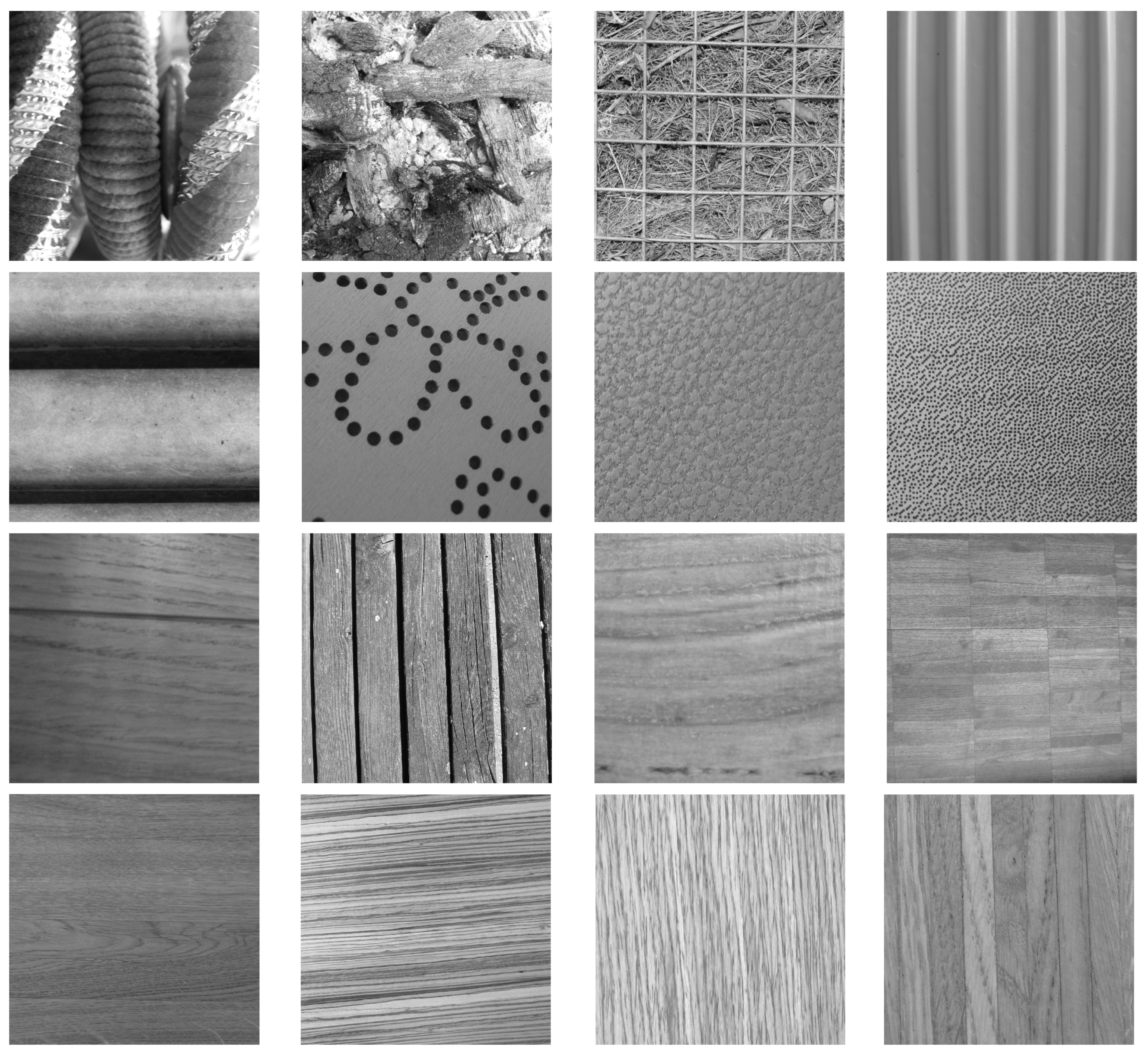
- Hofbauer, H.; Huber, S. Salzburg Texture Image Database (STex). 2019. Available online: https://wavelab.at/sources/STex/ (accessed on 1 October 2023).
- Bergillos, C. ts2vg 1.2.2. 2023. Available online: https://pypi.org/project/ts2vg/ (accessed on 1 October 2023).
- Ahmadvand, A.; Daliri, M.R. Invariant texture classification using a spatial filter bank in multi-resolution analysis. Image Vis. Comput. 2016, 45, 1–10. [Google Scholar] [CrossRef]
- Goyal, V.; Sharma, S. Texture classification for visual data using transfer learning. Multimedia Tools Appl. 2023, 82, 24841–24864. [Google Scholar] [CrossRef] [PubMed]
- Bello-Cerezo, R.; Bianconi, F.; Di Maria, F.; Napoletano, P.; Smeraldi, F. Comparative evaluation of hand-crafted image descriptors vs. off-the-shelf CNN-based features for colour texture classification under ideal and realistic conditions. Appl. Sci. 2019, 9, 738. [Google Scholar] [CrossRef]


| References | Purpose | Features | Model | Dataset | Accuracy (%) |
|---|---|---|---|---|---|
| [5,24] | Image texture classification | Statistical features, correlation | GLCM | Brodatz texture images | 99.043 |
| [7] | Texture classification | Wavelet statistical features | Wavelet transform | VisTex image dataset | Mean-97.80 |
| [10] | Texture classification | SNELBP features | SNELBP | KTH-TIPS | 95.97 |
| [1] | Texture characterization | GLCM Haralick | CatBoost classifier | Outex | 99.30 99.84% |
| [1] | Texture characterization | GLCM Haralick | CatBoost classifier LDA classifier | KTH-TIPS | 92.01 98.35 |
| [8] | Texture classification | Order statistics, histogram of configuration | Markov random field | Brodatz texture database | 87 |
| [9] | Color texture classification | Local class | GaRCIA | VisTex | Train-98.4 Test-89.2 |
| [11] | Texture descriptor quantify | BiT descriptor | SVM classifier | Salzburg Outex KTH-TIPS | 92.33 99.88 97.87 |
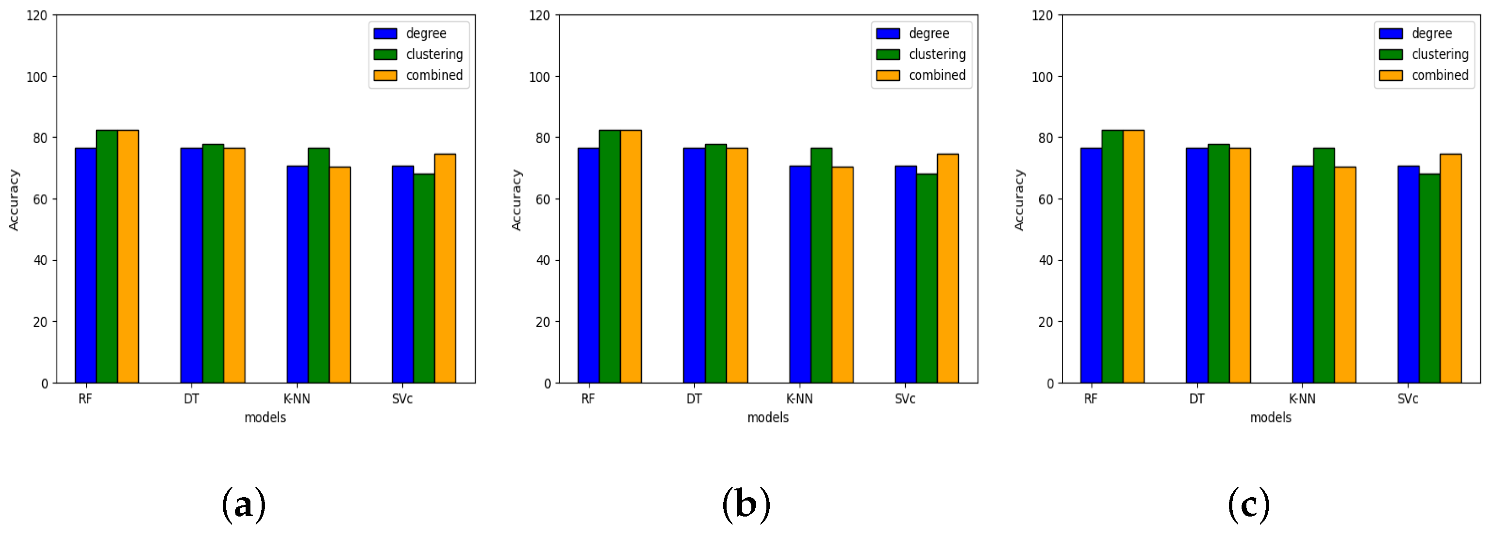
| Dataset | Graph | Feature | Machine Learning Classifier | |||
|---|---|---|---|---|---|---|
| RF (%) | DT (%) | KNN (%) | SVM (%) | |||
| Brodatz | INVG | Degree distribution | 80 | 80 | 60 | 60 |
| Clustering coefficient | 80 | 60 | 60 | 60 | ||
| Combination of both | 80 | 80 | 60 | 60 | ||
| IHVG | Degree distribution | 100 | 80 | 100 | 80 | |
| Clustering coefficient | 80 | 80 | 60 | 60 | ||
| Combination of both | 100 | 80 | 100 | 80 | ||
| INVG + IHVG | Degree distribution | 80 | 80 | 80 | 80 | |
| Clustering coefficient | 80 | 80 | 60 | 60 | ||
| Combination of both | 80 | 80 | 80 | 80 | ||
| Dataset | Graph | Feature | Machine Learning Classifier | |||
|---|---|---|---|---|---|---|
| RF (%) | DT (%) | KNN (%) | SVM (%) | |||
| STex | INVG | Degree distribution | 81.81 | 68.18 | 63.63 | 72.72 |
| Clustering coefficient | 82.35 | 70.58 | 70.58 | 88.23 | ||
| Combination of both | 76.47 | 76.47 | 70.58 | 70.58 | ||
| IHVG | Degree distribution | 63.63 | 63.64 | 68.18 | 54.54 | |
| Clustering coefficient | 76.58 | 76.47 | 68.88 | 58.88 | ||
| Combination of both | 82.35 | 77.77 | 76.47 | 68.18 | ||
| INVG + IHVG | Degree distribution | 81.81 | 77.27 | 68.81 | 72.72 | |
| Clustering coefficient | 82.35 | 76.47 | 68.18 | 72.27 | ||
| Combination of both | 82.35 | 76.47 | 70.47 | 74.71 | ||
| Dataset | Feature | Accuracy (%) |
|---|---|---|
| Brodatz | Gabor [24] | 43.429 |
| Gabor and GLCM [24] | 48.995 | |
| Hybrid feature [42] | 89.28 | |
| MobileNetV3 [43] | 99.67 | |
| InceptionV3 [43] | 99.33 | |
| IHVG (degree feature) | 100 | |
| IHVG (combination of degree and clustering) | 100 | |
| Salzburg | VGG-M-FC [44] | 82.5 |
| IHVG (combination of degree and clustering) | 82.35 | |
| VGG-VD-16-FC [44] | 83.3 | |
| INVG (clustering feature) | 88.23 |
Disclaimer/Publisher’s Note: The statements, opinions and data contained in all publications are solely those of the individual author(s) and contributor(s) and not of MDPI and/or the editor(s). MDPI and/or the editor(s) disclaim responsibility for any injury to people or property resulting from any ideas, methods, instructions or products referred to in the content. |
© 2023 by the authors. Licensee MDPI, Basel, Switzerland. This article is an open access article distributed under the terms and conditions of the Creative Commons Attribution (CC BY) license (https://creativecommons.org/licenses/by/4.0/).
Share and Cite
Ali, M.; Kumar, S.; Pal, R.; Singh, M.K.; Saini, D. Graph- and Machine-Learning-Based Texture Classification. Electronics 2023, 12, 4626. https://doi.org/10.3390/electronics12224626
Ali M, Kumar S, Pal R, Singh MK, Saini D. Graph- and Machine-Learning-Based Texture Classification. Electronics. 2023; 12(22):4626. https://doi.org/10.3390/electronics12224626
Chicago/Turabian StyleAli, Musrrat, Sanoj Kumar, Rahul Pal, Manoj K. Singh, and Deepika Saini. 2023. "Graph- and Machine-Learning-Based Texture Classification" Electronics 12, no. 22: 4626. https://doi.org/10.3390/electronics12224626