Adaptive Satellite Navigation Anti-Interference Algorithm Based on Inverse Cosine Function

Abstract

Contrasting the dilemma that the traditional time-domain least mean square (LMS) algorithm in the existing satellite navigation receiver anti-interference system cannot satisfy the convergence time is short and maintain a low level of steady-state error at the same time, an inverse cosine variable step size LMS algorithm (ICVS-LMS) is proposed. To begin with, the LMS algorithm, with a fixed step size focuses on its effectiveness in attenuating and suppressing interference signals, is analyzed, and then the proposed ICVS-LMS algorithm is analyzed. In conclusion, both the ICVS-LMS algorithm and the traditional algorithm are simulated and compared in terms of their effectiveness in suppressing interference in satellite navigation signals. The experimental results demonstrate that the improved algorithm significantly reduces convergence time while maintaining a small steady-state error. The improved algorithm demonstrates high robustness and an obvious suppression effect on interference signals. The anti-interference performance is 8.41–12.22% higher than that of the proposed algorithm.

1. Introduction

Satellite navigation signals need to travel a long distance to reach the ground to be received, and the ground reception signal power is weak, making it susceptible to many sorts of interference, whether deliberate or accidental [1,2,3,4,5]. For systems that rely on the global navigation satellite system (GNSS), even a small amount of interference might have disastrous results [6,7,8]. Satellite navigation system adopts spread spectrum communication technology and has certain anti-interference ability [9], but the receiver will malfunction if the interfering signal is too powerful and exceeds the system’s tolerance limitations [10]. Narrowband interference is a common form of interference signal utilized by a variety of interference equipment because it is simple to produce, cheap, and has a strong interference impact [11]. The three basic processing domains used for narrowband interference suppression are time, frequency, and combined domain [12,13,14,15]. One of the most popular methods for reducing narrowband interference in navigation receivers is time-domain anti-interference processing [16]. The time-domain anti-interference technology is now the more appropriate option for the future development trend in the BeiDou RDSS system, which has miniaturization and low power consumption as its aims [17]. Adaptive filters are primarily used in the time domain for interference suppression [18,19,20]. Adaptive algorithms modify their processes and parameters based on data traits, without full upfront information [21]. This ensures optimal convergence and maintains low error levels [22].

An algorithm with a good performance can ensure that the interference suppression effect is optimal, and the LMS algorithm is the classical algorithm [23]. Because the conventional LMS algorithm cannot accurately select the appropriate step size value according to the situation, the steady-state error and convergence speed cannot be optimized simultaneously. The problem of low applicability of a fixed step size LMS algorithm in many scenarios needs to be solved urgently. Qin et al. [24] proposed a filtering algorithm with a variable step size that can be automatically adjusted. The convergence and tracking effects are improved in the algorithm, but the error cannot be controlled in a small range. Zhang et al. [25] obtained a new function model by improving the Sigmoid function, which greatly shorten the convergence time without losing accuracy. Markala Karthik et al. [26] improved the LMS algorithm by using the hyperbolic secant cost function, which reinforces the system’s ability to cope with harsh environments and reduces the oscillation amplitude. D. Li et al. [27] proposed an improved LMS filtering algorithm with higher stability based on the hyperbolic tangent function. B. Jalal et al. [28] introduced a step size compensation factor according to the normalized sigmoid function. The algorithm automatically adjusts the step size value without changing the parameters, and the calculation is simple, but the convergence time of this method is too long, and the error value is large. Huo et al. [29] employed the inverse hyperbolic tangent function to construct a new formula, and achieved good results in system identification, noise removal, and other applications.

The above algorithm reduces the waiting time during the convergence period and maintains a low steady-state error value, but there are still problems, such as that both factors cannot be balanced, the computation is large, and the tracking performance is poor. To obtain a reasonable algorithm that can solve the existing problems, a novel LMS algorithm leveraging the inverse cosine function is proposed to enhance convergence speed and achieve a reduced error level. This algorithm demonstrates its efficacy in effectively suppressing narrow-band interference in satellite navigation signals.

The paper is structured into the following chapters: Section II explains the principle of suppressing interference using an LMS algorithm. Section III illustrates the improved ICVS-LMS algorithm and compares it with the three existing algorithms. In Section IV, the algorithm is applied to weaken the navigation interference signal, and the results prove the effectiveness of the algorithm. Finally, the conclusion expounds the main work content and contribution of this paper.

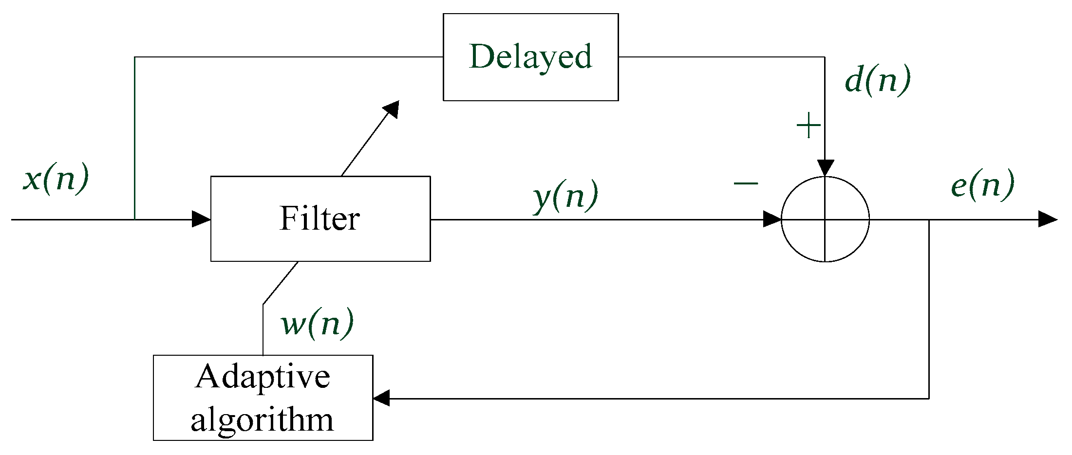
2. LMS Algorithm Interference Suppression Principle

The fundamental concept of an adaptive filter for interference suppression is depicted in Figure 1, which illustrates the core principle behind its operation. $x(n)$ is the received signal of the receiver, including the satellite navigation signal, narrowband interference signal, and noise signal, $d(n)$ denotes the delay of $x(n)$ which is used as the reference signal of the adaptive filter, $y(n)$ is the output of the adaptive filter after processing, $e(n)$ denotes that the difference between the output signal and the reference signal is the error signal, and the error signal automatically adjusts the tap weight $w(n)$ of the adaptive filter according to the adaptive algorithm [30]. The input satellite navigation signals and noise signals are time domain broadband signals with small sample time delay correlation, but the correlation of the narrowband interference sample value is much stronger than that of the broadband signal, and the current signal value can be estimated using the past signal value [31]. Depending on the correlation, the estimated signal of narrowband interference can be generated through an adaptive filter, canceling it out from the input signal to achieve narrowband interference suppression [32].

The receiver receives the satellite navigation signal and down-converts it to obtain the intermediate frequency signal (IF signal), which is digitally sampled by the analog-to-digital convert (ADC) to obtain the input signal as follows:

$$x(n)=s(n)+j(n)+n(n)$$

(1)

where $s(n)$ is the received satellite navigation sign, $j(n)$ is the narrowband interference sign and $n(n)$ is the noise sign. The reference signal $d(n)$ is the delay of the input signal $x(n)$. $x(n)$ and $d(n)$ will cancel the signal with correlation and the signal without correlation will be unaffected, where:

$$e(n)=d(n)-y(n)$$

(2)

The LMS algorithm replaces the mean square error (MSE) $E({\left|e(n)\right|}^2)$ by a single sample of data ${\left|e(n)\right|}^2$ [33], and the gradient estimate during the iteration needs to satisfy the following [34]:

$$\begin{array}{l}\stackrel{\wedge }{\nabla }(n)=\partial {\left|e(n)\right|}^2/\partial W(n)\\ =\partial \{{\left|x(n)\right|}^2+W^H(n)X(n)W(n)\\ -2\mathrm{Re}[x(n)X^T(n)W(n)]\}/\partial W(n)\\ =2W^H(n)X(n)W(n)-2x(n)X(n)\\ =-2e(n)X(n)\end{array}$$

(3)

Therefore, the filter weight coefficient vector iterative formula of the LMS algorithm is as follows [34]:

$$W(n+1)=W(n)+2\mu e(n)X(n)$$

(4)

where $W(n)$ is the filter coefficient vector, $X(n)$ is the input vector, $e(n)$ is the error signal, and $\mu$ is the key to determine the convergence and error level of LMS algorithm, which can reduce the time required for convergence and limit the error in a small range [35].

The main implementation process of the LMS algorithm is as follows:

$$y(n)=\mathit{W}{(n)}^H\mathit{X}(n)$$

(5)

$$e(n)=d(n)-y(n)$$

(6)

$$\mathit{W}(n+1)=\mathit{W}(n)+2\mu (n)e(n)\mathit{X}(n)$$

(7)

where $\mathit{X}(n)$ is the input signal at moment $n$, $\mathit{W}(n)$ is the weight coefficient of the filter at moment $n$, and $\mu (n)$ is the iteration step size factor. The condition that the LMS algorithm must satisfy to achieve the convergence effect is: $0<\mu <1/{\lambda }_m$, and ${\lambda }_m$ is the maximum eigenvalue of the filter input signal autocorrelation matrix.

3. Improved Variable Step Size LMS Algorithm

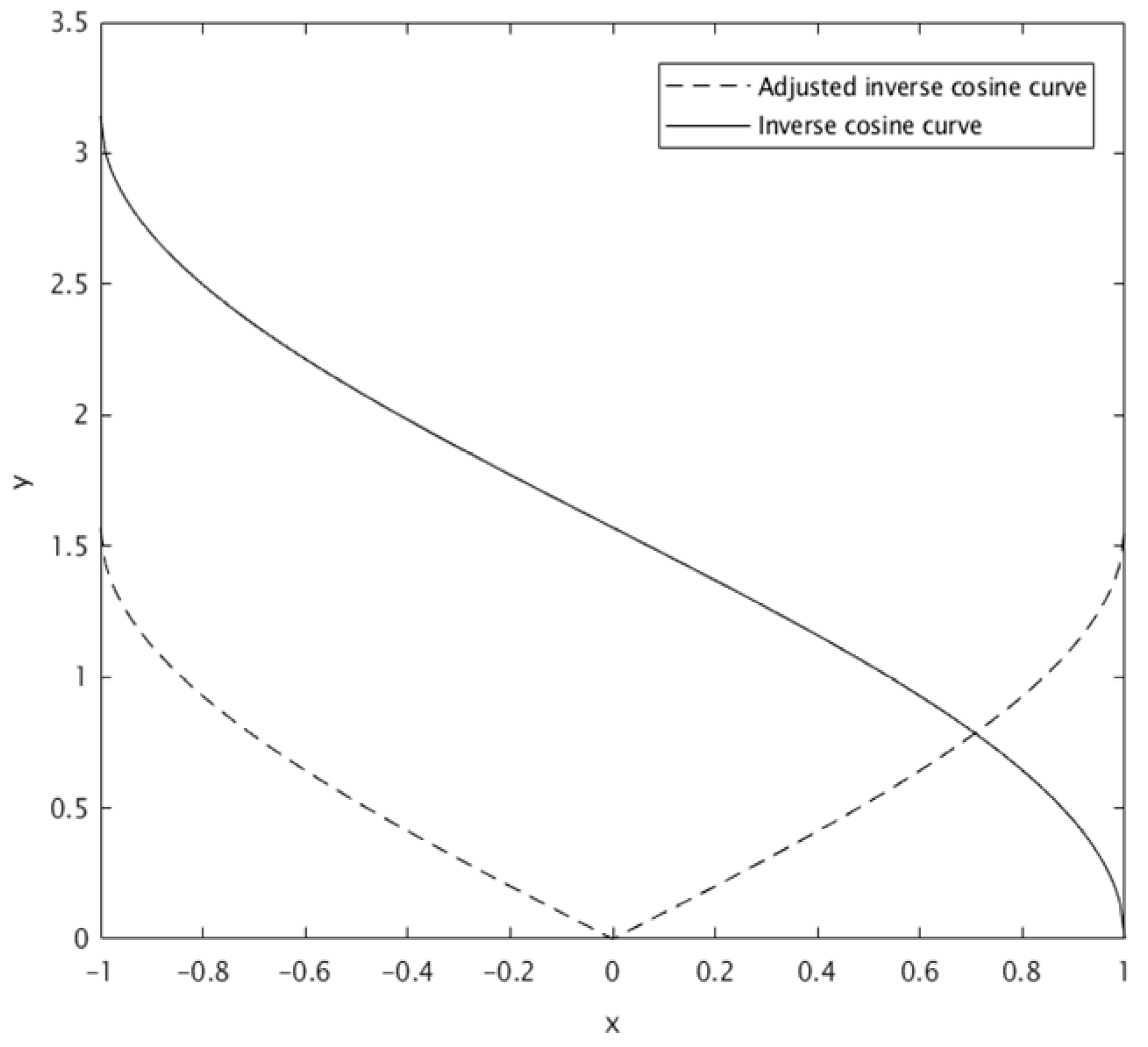
3.1. Improved Inverse Cosine Variable Step Size LMS Algorithm

Achieving convergence in a short time while maintaining a low level of steady-state error are two crucial evaluation metrics of the algorithm and, in order to achieve both, experts and scholars have studied and proposed various new algorithms [36]. When the variable step size LMS algorithm has not yet reached the convergence state, it will choose an outsize step size value to shorten the time spent on convergence. When the algorithm enters the convergence period, the step size value gradually becomes smaller, maintaining a low level of error value and avoiding missing the best point.

The calculation formula of step length is a key part used to enhance the application effect of the algorithm [37], and the new step length calculation formula is constructed through functions, which are widely chosen as sigmoid functions, hyperbolic tangent functions, exponential functions, inverse tangent functions, etc.

In the pursuit of enhancing conventional algorithms, one frequently encountered path for improvement involves the utilization of the sigmoid function. This pathway holds broader applicability and often yields favorable outcomes. To underscore the merits of the algorithm introduced in this manuscript, we have opted to juxtapose it with three prominent algorithms from pertinent references. These selections have been chosen to highlight the algorithm’s advantages in comparison to both traditional and currently popular algorithms.

Innovatively, reference [38] employed the logarithmic function to construct the step size formula of the algorithm and obtained the improved LVS-LMS algorithm with strong stability. The new step size calculation formula is as follows:

$$\mu (n)=b\log (a{\left|e(n)\right|}^m)$$

(8)

Reference [39] skillfully used the Versiera function to obtain the step size calculation method and obtained the VVS-LMS algorithm with superior performance. The new step size formula is as follows:

$$\mu (n)=a[1-\frac{1}{b{e}^2(n)+1}]$$

(9)

Reference [40] integrated the normal distribution curve into the construction of the step size formula in order to improve the LMS algorithm, and the NDVS-LMS algorithm with stable performance is obtained. The improved step size formula is as follows:

$$\mu (n)=c(1-\exp (-a{\left|e(n)\right|}^b))$$

(10)

In this paper, according to the LMS algorithm step factor adjustment rules, it is possible to use the inverse cosine function to make the size of the step size change according to the different convergence states of the algorithm. The expression of the inverse cosine function is as follows:

$$y=\arccos (x)$$

(11)

The function is defined over the interval (−1, 1), exhibiting properties of an odd function characterized by a monotonically decreasing trend within this range. The corresponding graphical representation is depicted as the dashed line in Figure 2. Upon manipulation of the independent variable in Equation (11), the resultant function takes the following form:

$$y=\left|\arccos (x)-\frac{\pi }{2}\right|$$

(12)

The plotted function resulting from Equation (12) is represented by the solid line in Figure 2. The visual analysis of the graph reveals a conformity to the algorithm’s step size adjustment mechanism, as evidenced by the gradual decline in slope with the increase in the independent variable. This trend signifies that during the initial convergence stages, the step size is larger, becoming smaller as convergence nears completion, and exhibiting gradual adjustments when the error approaches zero. Therefore, by employing Formula (3), we can establish the relationship between step size and error in the following manner:

$$\mu (n)=\left|\arccos (e(n))-\frac{\pi }{2}\right|$$

(13)

According to Expression (13), and also for better control adjustment of the function shape, the parameters $\alpha$, β, $\gamma$, and $m$ are introduced to obtain the improved variable step size function, as follows:

$$\mu (n)=\frac{-2\arccos [\alpha \left|e{(n)}^{\gamma }\right|]+\pi }{m\arccos [\alpha \left|e{(n)}^{\beta }\right|]+2}$$

(14)

The normalization algorithm is used in the iterative formula for the weighting coefficients, and the parameter $\xi$ is introduced to avoid a too small value of $X^T(n)X(n)$, which is the minimum value to be neglected.

In summary, the step size formula of the ICVS-LMS algorithm is enhanced by incorporating the inverse cosine function and introducing a parametric control function shape, aimed at better adhering to the algorithm’s application rules [41]. The golden key steps of the ICVS-LMS algorithm, which utilizes the inverse cosine function, can be summarized as follows:

$$e(n)=d(n)-W^T(n)X(n)$$

(15)

$$\mu (n)=\frac{-2\arccos [\alpha \left|e{(n)}^{\gamma }\right|]+\pi }{m\arccos [\alpha \left|e{(n)}^{\beta }\right|]+2}$$

(16)

$$W(n+1)=W(n)+\frac{2\mu (n)e(n)X(n)}{\xi +X^T(n)X(n)}$$

(17)

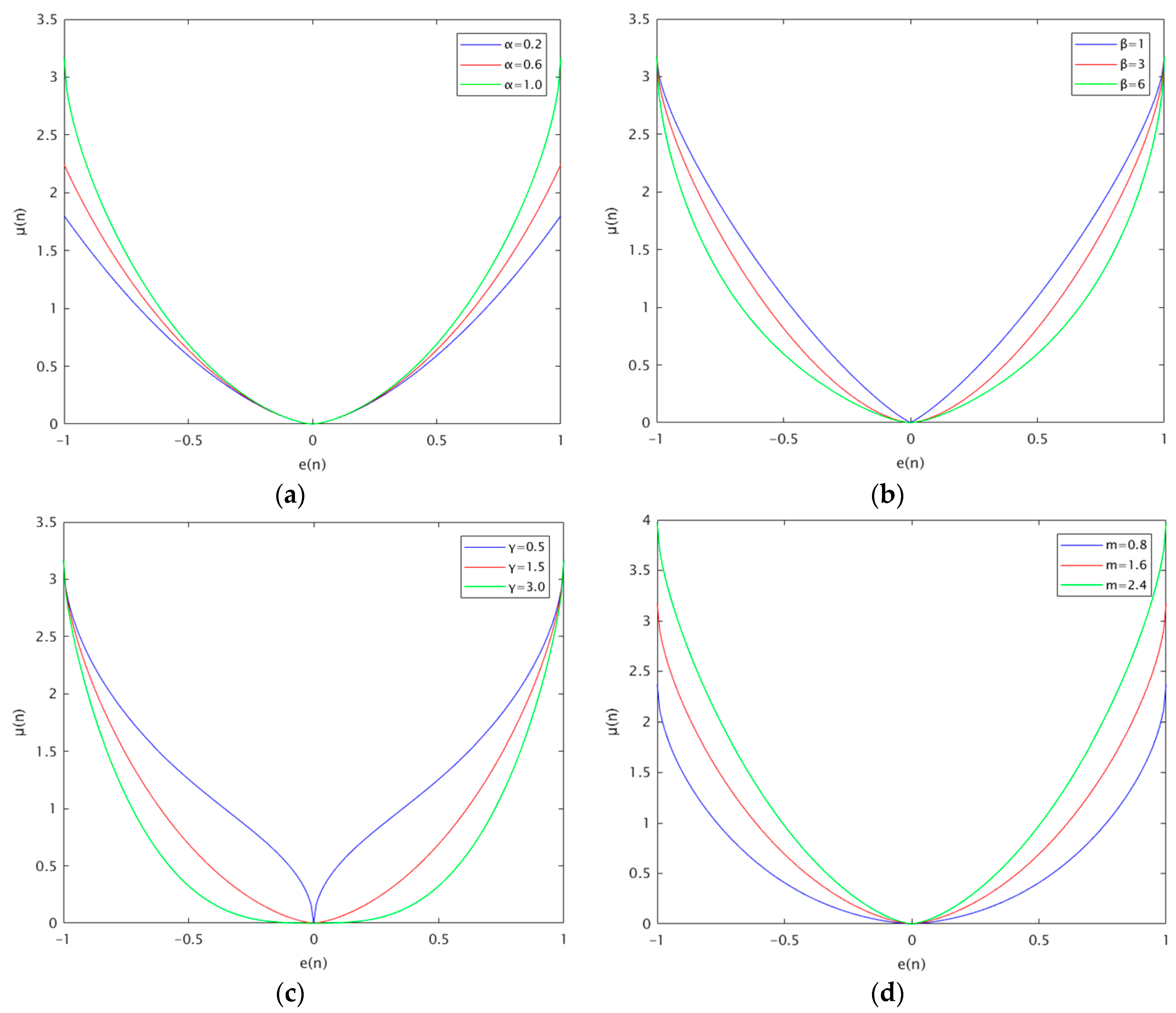
3.2. Influence of Parameters on The ICVS-LMS Algorithm

To develop a better understanding of the four additional parameters and their impact on the performance of the function, it is necessary to examine their relationship more closely, and an analysis is conducted on the varying values of these parameters.

The curves in Figure 3a are when $\alpha$ is taken as 0.2, 0.6, 1.0, $\beta =6$, $\gamma =1.5$, and $m=1.6$, respectively. With the increase value of $\alpha$, the convergence also accelerates, and the influence of parameter $\alpha$ on the convergence speed diminishes as the algorithm reaches its later stages. Considering the whole convergence process of the algorithm, $\alpha =1.0$ is chosen.

The curves in Figure 3b are when $\beta$ is taken as 1, 3, 6, $\alpha =1.0$, $\gamma =1.5$ and $m=1.6$, respectively. With the increase value of $\beta$, the algorithm can converge rapidly in the initial state, and the better stability; with the decrease value of $\beta$, the algorithm exhibits slow convergence during its initial stage, and the speed is fast when it tends to be stable, and increasing the step size to a larger value, which compromises the stability of the system. When $\beta =3$ and $\beta =6$, it is relatively stable in the later stage of convergence. When $\beta =6$, the speed is faster in the early stage. Based on the above factors, $\beta =6$ is selected.

The curves in Figure 3c are when $\gamma$ is taken as 0.5, 1.5, 3.0, $\alpha =1.0$, $\beta =6$, and $m=1.6$, respectively. With the increase in the value of $\gamma$, the algorithm can converge quickly in the initial state. However, when the error $e(n)$ is non-zero, the step size factor $\mu (n)$ becomes zero, leading to the algorithm taking more time to enter the convergence state. When the value of $\gamma$ is small, the shape of the curve deforms too fast, and it is likely to lose the best point. Based on the above factors, $\gamma =1.5$ is selected.

The curves in Figure 3d are when $m$ is taken as 0.8, 1.6, 2.4, $\alpha =1.0$, $\beta =6$, and $\gamma =1.5$, respectively. With the increase in the value of $m$, the algorithm can obtain faster convergence at the beginning, but it will bring bad error values. When the value of $m$ is small, the error value can be kept in a smaller range, but it takes a long time to converge. Through the above comparison, $m=1.6$ is selected.

4. Simulation Analysis

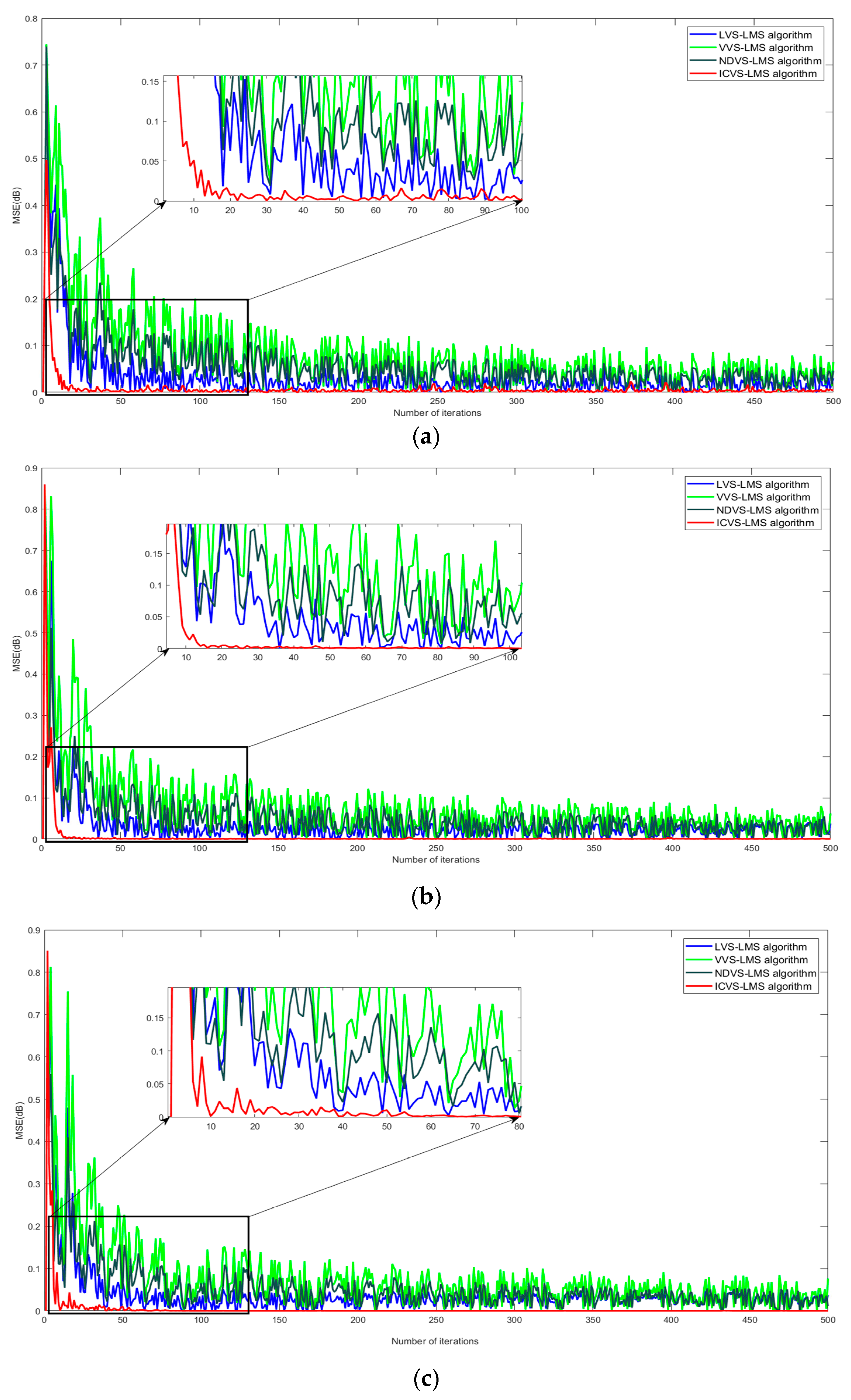
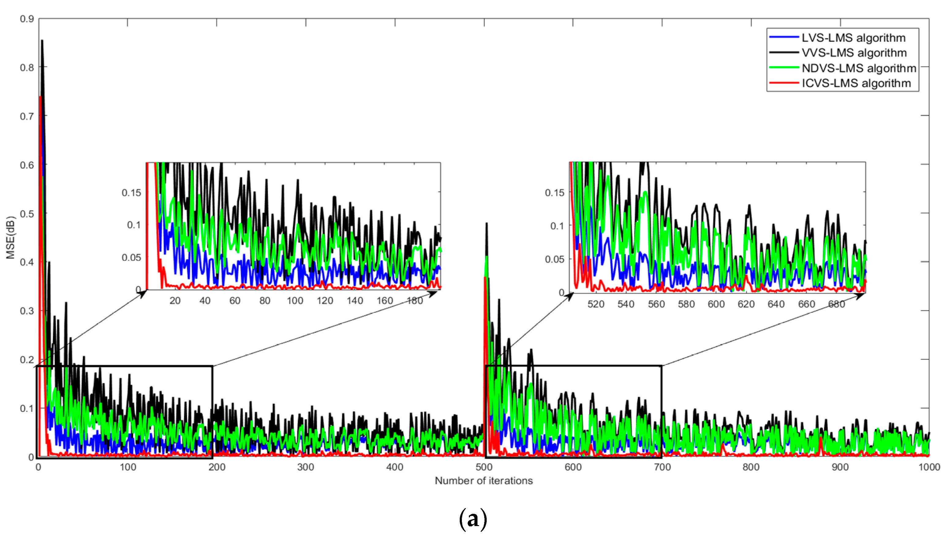
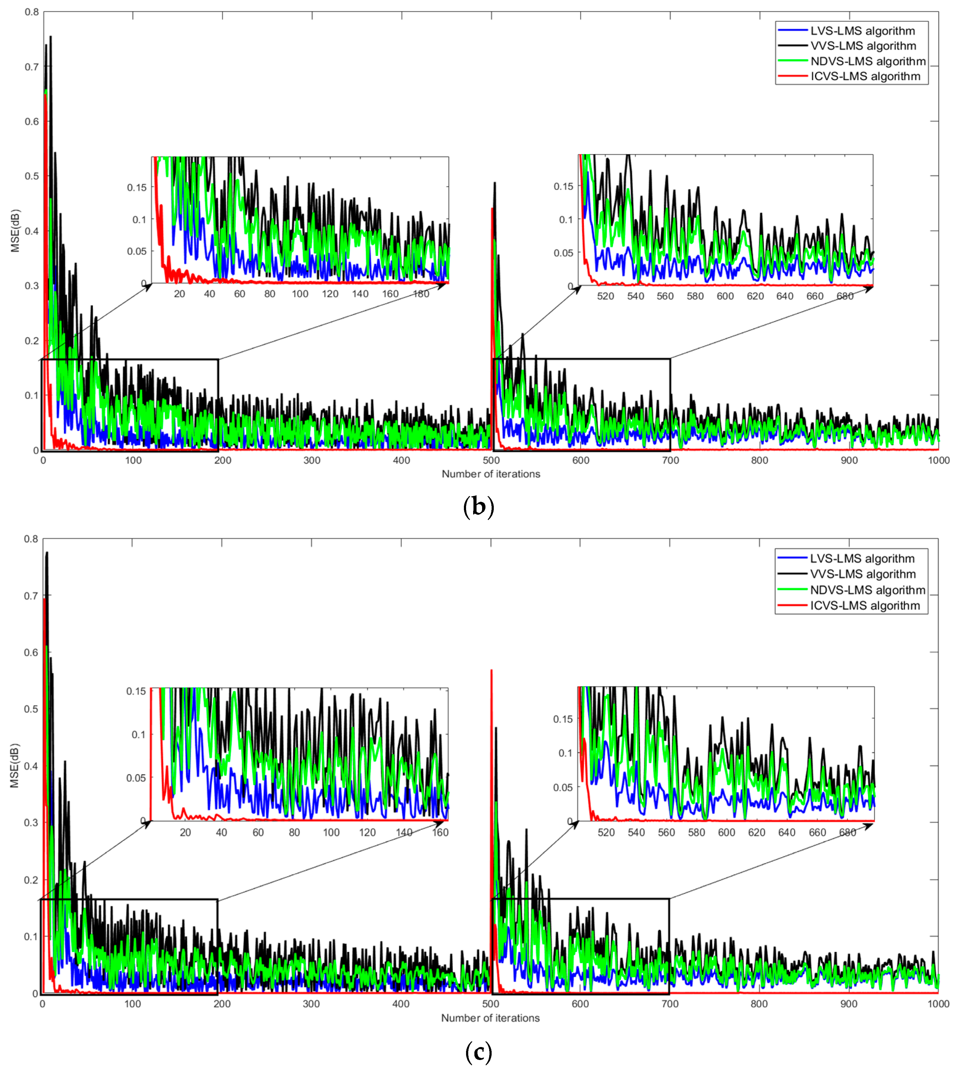
4.1. Performance Verification of The Improved Variable Step Size Algorithm

To showcase the benefits of the ICVS-LMS algorithm in iterative convergence times, steady-state error control, and tracking capability, as well as the impacts of parameters $\alpha$, $\beta$, $\gamma$, and $m$ on the properties of the algorithm, the algorithm is simulated in MATLAB R2017b software under the following conditions [20]: let the order of the adaptive filter $M=2$, and the unknown system is a transverse FIR structure. The tapping coefficients are ${\mathit{W}}^{*}={\left[0.8,0.5\right]}^T$. At the 500th iteration, the system is time-varying, and the tap coefficients change abruptly to ${\mathit{W}}^{*}={\left[0.4,0.2\right]}^T$. Assuming that the reference input signal $\mathit{X}(n)$ and the interference noise $v(n)$ are both Gaussian white noise with zero mean, the variance of the reference input signal $\mathit{X}(n)$ is 1 and the variance of the interference noise $v(n)$ is 0.04. The number of sampling points of the system is set to 1000, and 200 independent simulations are performed for each algorithm to achieve the statistical average and the learning curve against different signal-to-noise ratio (SNR) backgrounds.

Figure 4 illustrates the convergence curves of the four algorithms. Looking at the figure, it is evident that when faced with three different noise backgrounds (SNR values of 20, 30, and 40, respectively), the VVS-LMS algorithm requires the highest number of iterations to converge. On the other hand, the proposed ICVS-LMS algorithm demonstrates the fewest iterations during the initial stage of convergence while maintaining a relatively low steady-state error, which can effectively address the challenges of accelerating convergence and handling large errors encountered in the LMS algorithm. The steady-state error is effectively suppressed at a low level by the proposed ICVS-LMS algorithm under three noise backgrounds, and the benefits of lower iterative convergence times and low error of the proposed ICVS-LMS algorithm become more obvious as the SNR continues to increase.

To underline the superiority of the proposed ICVS-LMS algorithm, we compare the convergence performance of the four algorithms across different signal-to-noise ratio (SNR) levels by examining their respective iteration counts, as detailed in

Table 1. Comparison of iteration times under different signal-to-noise ratios.

SNR (dB)	LVS-LMS Algorithm	VVS-LMS Algorithm	NDVS-LMS Algorithm	ICVS-LMS Algorithm
20	170	380	360	30
30	200	400	380	60
40	260	430	450	100

. When the SNR is set at 20 dB, the ICVS-LMS algorithm achieves convergence within just 30 iterations, outperforming the LVS-LMS algorithm, which requires 170 iterations, and significantly surpassing both the VVS-LMS and NDVS-LMS algorithms, both of which demand more than 350 iterations. At an increased SNR of 30 dB, the ICVS-LMS algorithm attains convergence in 60 iterations, while the LVS-LMS algorithm necessitates 200 iterations. Moreover, the VVS-LMS and NDVS-LMS algorithms exhibit considerably higher iteration counts at 400 and 380 iterations, respectively. As the SNR escalates to 40 dB, the ICVS-LMS algorithm achieves convergence within 100 iterations, once again surpassing the LVS-LMS algorithm’s requirement of 260 iterations. Additionally, the VVS-LMS and NDVS-LMS algorithms maintain convergence behavior above 400 iterations.

To validate the traceability and convergence capability of the proposed ICVS-LMS algorithm, as well as its comparison against existing algorithms, we tested the algorithm when dealing with time-varying system occurrences. When the algorithm iterative process reaches 500 iterations, the unknown system occurs in a time-varying manner, and Figure 5 shows the algorithm’s ability to cope with the time-varying system under different SNR.

Based on the information presented in Figure 5, it is evident that the proposed ICVS-LMS algorithm can achieve rapid convergence in approximately 50 iterations, even when dealing with an unknown system that exhibits time-varying characteristics, while the LVS-LMS algorithm, the VVS-LMS algorithm, and the NDVS-LMS algorithm need about 100, 350, and 400 iterations to reach convergence, respectively, while the proposed ICVS-LMS algorithm exhibited a rapid convergence speed while simultaneously sustaining a minimal level of steady-state error, with obvious advantages and better coping ability.

4.2. Navigation Interference Suppression Effect Analysis

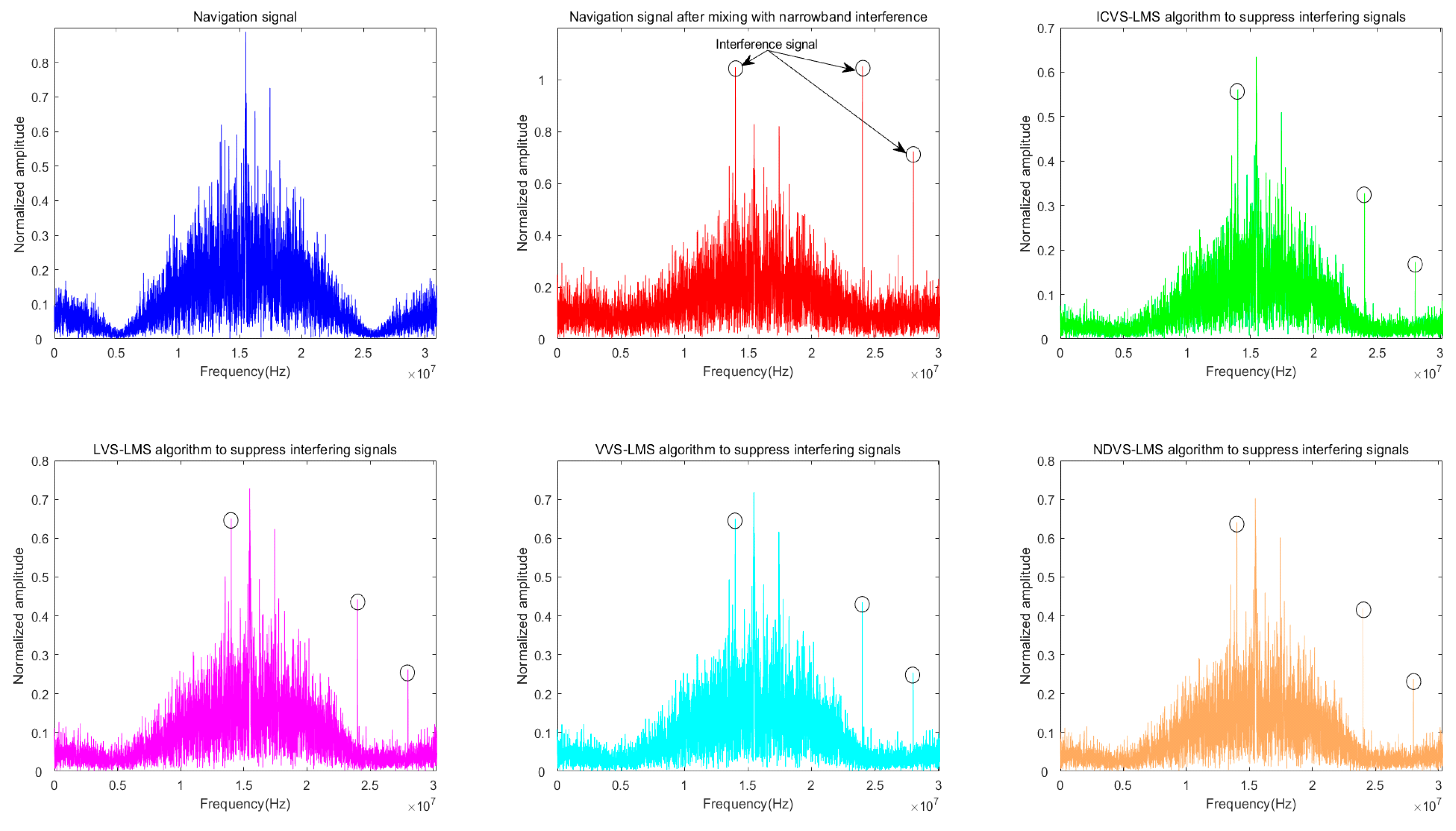
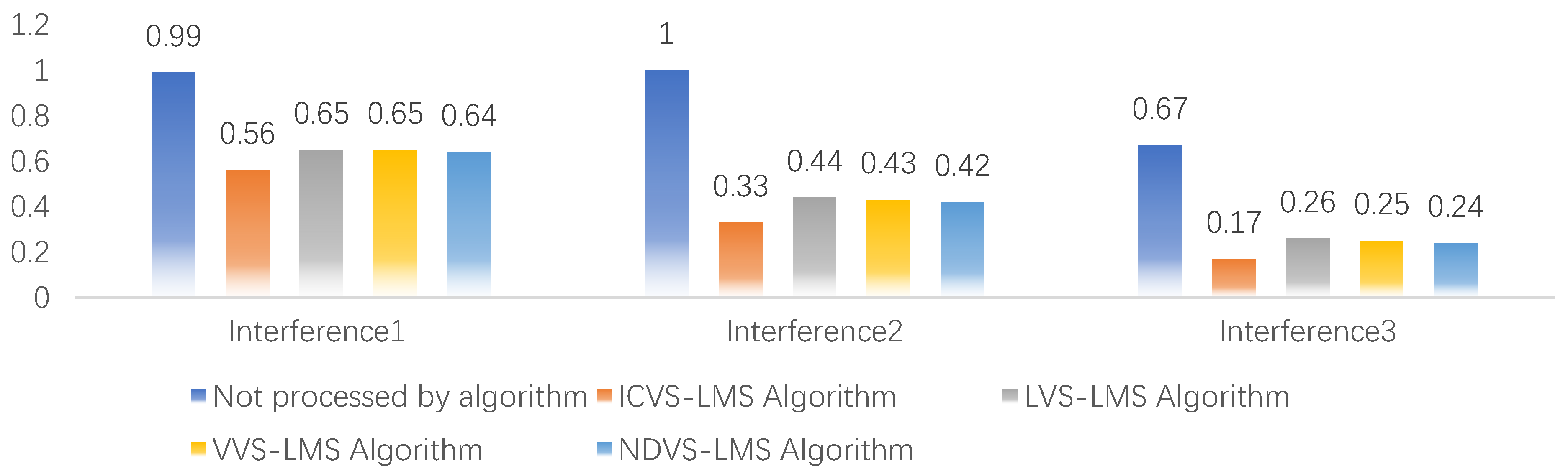
4.2.1. Simulation Verification of Interference Suppression Performance

Three interfering signals are added to the satellite navigation signal for the suppression simulation. The B1I satellite signal power is −160 dBW, the IF signal bandwidth is 4.092 MHz, the center frequency is 1.546 MHz, the sampling frequency is 20 MHz, three narrowband interfering signals are added with frequencies of 1.4 MHz, 2.4 MHz, and 2.8 MHz, and they dry signal ratio is 50 dB. Four algorithms are employed for the purpose of attenuating interfering signals and retrieving the original satellite navigation signal. By effectively mitigating the interference present in the satellite navigation signal, these algorithms successfully suppress the interference and yield a power spectrum that accurately represents the reduced interference level.

Figure 6 shows the spectrum of the normal satellite navigation signal, the satellite navigation signal joined with the interference, the proposed ICVS-LMS algorithm, the LVS-LMS algorithm, the VVS-LMS, algorithm and the NDVS-LMS algorithm when suppressing the three interfering signals. According to Figure 6, it is evident that the spectral line of the narrowband interference exhibits a considerably greater magnitude compared to that of the normal signal, and the four algorithms have inhibitory effects on narrowband interference signals. Compared with the three existing algorithms in the literature, the adaptive filtering using the ICVS-LMS algorithm proposed in this paper is more effective in suppressing the three narrowband interfering signals.

Figure 7 displays the amplitude comparison diagram of the three interference signals processed by different algorithms. After implementing the algorithm proposed in this paper, the amplitude of the three interference signals is reduced compared to that of other algorithms and maintains a consistently low level.

Table 2. Comparison of interference suppression performance of the four algorithms.

Interference Signals	LVS-LMS Algorithm	VVS-LMS Algorithm	NDVS-LMS Algorithm	ICVS-LMS Algorithm
Interference1	38.86%	37.99%	38.77%	46.40%
Interference2	57.98%	58.71%	60.19%	69.13%
Interference3	63.88%	65.09%	67.15%	76.10%

shows the comparison of the suppression weakening of interference signals between the ICVS-LMS algorithm and the existing algorithms. Regarding interference suppression 1, the three existing literature algorithms exhibit similar suppression capabilities, hovering around 38%. In contrast, this paper’s algorithm achieves a notable 46.4% suppression rate, demonstrating superior performance in weakening and mitigating interference signals compared to the other three algorithms; in the suppression of interference 2, the lowest suppression ability of the LVS-LMS algorithm is 57.98%. The VVS-LMS and the NDVS-LMS algorithms interference suppression abilities are slightly improved compared to the LVS-LMS algorithm, but the effect is limited, while the ICVS-LMS algorithm can improve the interference suppression ability by more than 10% compared to the lowest level; in the suppression of interference 3, the suppression ability of the four algorithms is improved compared with that in interference 1 and 2, and the interference suppression ability of the algorithm in this paper is still the most advantageous among the four algorithms.

In summary, the suppression effect of the proposed ICVS-LMS algorithm on all three interfering signals is better than the three existing algorithms, and the ability to suppress interference is improved by 8.41–12.22%, which fully proves the superiority of the algorithm’s performance in interference suppression.

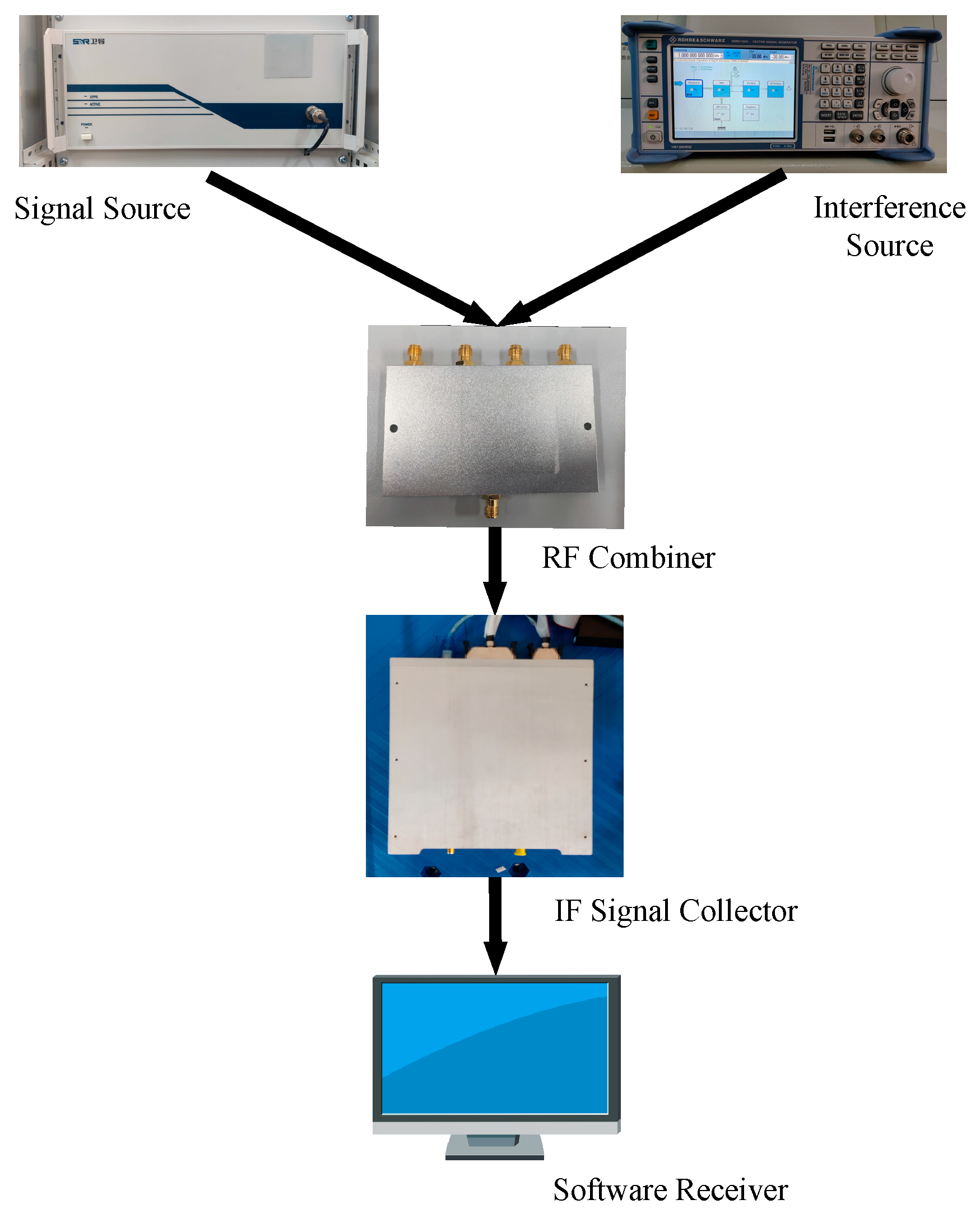
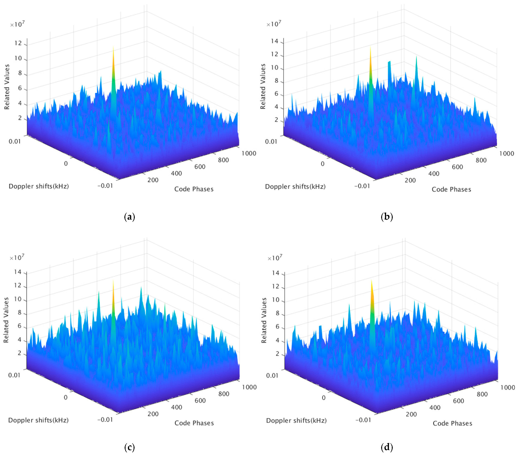
4.2.2. Experimental Verification of Interference Suppression Performance

To verify the suppression effect of the algorithm on navigation interference signals, the algorithm anti-interference performance verification hardware system structure is shown in Figure 8, mainly using the satellite navigation signal simulator to generate normal satellite navigation signals and the vector signal generator to generate interference signals through the combiner into the IF signal collector, where the collected IF signal is subjected to a series of operations, such as capture, tracking, positioning, and decoding, after the anti-interference algorithm in the software receiver [42]. The signal source is the NSS8900 simulation source of Hunan Satellite Navigation Company (Changsha, China), and the interference source is the SMBV100 A Vector Signal Generator produced by Rohde & Schwarz Company (Munich, Germany).

The satellite capture results serve as a more intuitive indicator to assess the algorithm’s effectiveness in mitigating and suppressing interference signals. In the simulation experiments, the SNR of the navigation signal is deliberately set to −20 dB. Figure 9 illustrates the acquisition outcomes of four distinct algorithms after they have processed the signals received by the receiver. The orange peak represents the acquisition peak of the navigation signal.

The simulation results in Figure 9a reveal a distinct peak in the satellite capture outcome from this algorithm. The adjacent interference peaks have been effectively suppressed, minimizing their impact on the navigation signal. This reduction in interference during capture safeguards against potential disruptions to the target signal, ensuring the receiver’s accurate capture of the navigation signal and decoding of precise navigation information.

The Figure 9b–d show that the existing algorithm is less effective in suppressing interference when capturing satellite signals, and although there are peaks in the navigation signal, there are more interference peaks in the surrounding area, which can easily interfere with the target navigation signal in the process of capturing, thus, resulting in false capture and affecting the subsequent tracking and positioning solution. It shows that the proposed ICVS-LMS algorithm has a more effective interference suppression ability.

5. Conclusions

This paper proposes an LMS time-domain algorithm based on the inverse cosine function, aiming to address the vulnerability of satellite navigation receivers to narrowband interference. The algorithm exhibits fast convergence, enhanced stability, and a lower steady-state error compared to existing algorithms, thereby improving the receiver’s immunity to interference. In satellite navigation signal narrowband interference suppression experiments, the algorithm in this paper significantly outperformed existing algorithms in suppressing the added narrowband interference signals. Upon capturing the navigation signal, the algorithm proposed in this paper significantly enhances the prominence of the signal’s peak while effectively reducing interference peaks. As a result, the risk of incorrect navigation signal capture due to excessive interference is mitigated, leading to improved capture accuracy. The research conducted in this paper establishes a crucial theoretical foundation for mitigating narrowband interference within navigation receiver systems. Moreover, its applicability extends to other domains, such as speech processing and equipment noise reduction, catering to scenarios that require the attenuation or elimination of noise.

References

1. Wei, Q.; Gao, Y.; Chen, X.; Huang, Z.; Kuang, L. Spatial Filtering for Interference Mitigation in High-Altitude Spaceborne GNSS Receivers. IEEE Trans. Aerosp. Electron. Syst. 2023, 59, 274–291. [Google Scholar] [CrossRef]
2. Huang, L.; Lu, Z.; Xiao, Z.; Ren, C.; Song, J.; Li, B. Suppression of Jammer Multipath in GNSS Antenna Array Receiver. Remote Sens. 2022, 14, 350. [Google Scholar] [CrossRef]
3. Merwe, J.; Cortés, I.; Garzia, F.; Rügamer, A.; Felber, W. Exotic FMCW Waveform Mitigation with an Advanced Multi-Parameter Adaptive Notch Filter (MPANF). In Proceedings of the 35th International Technical Meeting of the Satellite Division of the Institute of Navigation (ION GNSS+ 2022), Denver, Colorado, 19–23 September 2022; pp. 3783–3819. [Google Scholar]
4. Chen, X.; He, D.; Yan, X.; Yu, W.; Truong, T.-K. GNSS Interference Type Recognition with Fingerprint Spectrum DNN Method. IEEE Trans. Aerosp. Electron. Syst. 2022, 58, 4745–4760. [Google Scholar] [CrossRef]
5. Lu, Z.; Chen, F.; Xie, Y.; Sun, Y.; Cai, H. High Precision Pseudo-Range Measurement in GNSS Anti-Jamming Antenna Array Processing. Electronics 2020, 9, 412. [Google Scholar] [CrossRef]
6. Cao, Y.; Bai, H.; Jin, K.; Zou, G. An GNSS/INS Integrated Navigation Algorithm Based on PSO-LSTM in Satellite Rejection. Electronics 2023, 12, 2905. [Google Scholar] [CrossRef]
7. Kim, H.; Lee, J.; Oh, S.H.; So, H.; Hwang, D.-H. Multi-Radio Integrated Navigation System M&S Software Design for GNSS Backup under Navigation Warfare. Electronics 2019, 8, 188. [Google Scholar]
8. Chien, Y.R.; Chen, P.Y.; Fang, S.H. Novel Anti-Jamming Algorithm for GNSS Receivers Using Wavelet-Packet-Transform-Based Adaptive Predictors. IEICE Trans. Fundam. Electron. Commun. Comput. Sci. 2017, E100-A, 602–610. [Google Scholar] [CrossRef]
9. Wang, P.; Cetin, E.; Dempster, A.G.; Wang, Y.; Wu, S. GNSS Interference Detection Using Statistical Analysis in the Time-Frequency Domain. IEEE Trans. Aerosp. Electron. Syst. 2018, 54, 416–428. [Google Scholar] [CrossRef]
10. Hwang, S.S. Adaptive Algorithms for a GPS Interference Suppression Receiver and a Sparse Reconfigurable Adaptive Filter. Ph.D. Thesis, University of California, Santa Barbara, CA, USA, 2006. [Google Scholar]
11. Džunda, M.; Melníková, L. The Influence of Narrowband Interference on DME System Operation. Aerospace 2023, 10, 663. [Google Scholar] [CrossRef]
12. Li, X.; Chen, F.; Lu, Z.; Liu, Z.; Ou, G. Overview of Anti-Jamming Technology Based on GNSS Single-Antenna Receiver. In Proceedings of the ICGDA 2020: Proceedings of the 2020 3rd International Conference on Geoinformatics and Data Analysis, New York, NY, USA, 15–17 April 2020; pp. 96–104.
13. Mosavi, M.R.; Shafiee, F. Narrowband Interference Suppression for GPS Navigation Using Neural Networks. GPS Solut. 2016, 20, 341–351. [Google Scholar] [CrossRef]
14. Zou, M.; Chen, J.; Luo, J.; Hu, Z.; Chen, S. Equilibrium Approximating and Online Learning for Anti-Jamming Game of Satellite Communication Power Allocation. Electronics 2022, 11, 3526. [Google Scholar] [CrossRef]
15. Wang, P.; Wang, Y.; Cetin, E.; Dempster, A.G.; Wu, S. GNSS Jamming Mitigation Using Adaptive-Partitioned Subspace Projection Technique. IEEE Trans. Aerosp. Electron. Syst. 2019, 55, 343–355. [Google Scholar] [CrossRef]
16. Shi, K.; Jia, Y.; Fu, S.; Cao, Z.; Chen, P. Adaptive Narrowband Antijam Method for Satellite Navigation. In Proceedings of the 2018 International Conference on Electromagnetics in Advanced Applications (ICEAA), Cartagena, Colombia, 10–14 September 2018; pp. 687–690. [Google Scholar]
17. Li, X.H. Research on Time Domain Adaptive Anti-Jamming Technology for Satellite Navigation. Master’s Thesis, National University of Defense Technology, Changsha, China, 2020. [Google Scholar]
18. Liu, W.; Lu, Z.; Wang, Z.; Li, X.; Li, Z.; Xiao, W.; Ye, Z.; Wang, Z.; Song, J.; Qiao, J.; et al. Sidelobes Suppression for Time Domain Anti-Jamming of Satellite Navigation Receivers. Remote Sens. 2022, 14, 5609. [Google Scholar] [CrossRef]
19. Wang, S.; Wang, S.; Sun, X. A Multi-Scale Anti-Multipath Algorithm for GNSS-RTK Monitoring Application. Sensors 2023, 23, 8396. [Google Scholar] [CrossRef]
20. Chien, Y.-R. Wavelet Packet Transform-Based Anti-Jamming Scheme with New Threshold Selection Algorithm for GPS Receivers. J. Chin. Inst. Eng. 2018, 41, 181–185. [Google Scholar] [CrossRef]
21. Song, J.; Lu, Z.; Liu, Z.; Xiao, Z.; Dang, C. A Review of Time Domain Adaptive Anti-Jamming Techniques for Satellite Navigation. Syst. Eng. Electron. Technol. 2023, 45, 1164–1176. [Google Scholar]
22. Kwong, R.H.; Johnston, E.W. A Variable Step Size LMS Algorithm. IEEE Trans. Signal Process. 1992, 40, 1633–1642. [Google Scholar] [CrossRef]
23. Jiang, T.; Liu, J.; Peng, C.; Wang, S. Laboratory Test of a Vehicle Active Noise-Control System Based on an Adaptive Step Size Algorithm. Appl. Sci. 2023, 13, 225. [Google Scholar] [CrossRef]
24. Qin, J.; Ouyang, J. A New Variable Step Length LMS Adaptive Filtering Algorithm. J. Data Acquis. Process. 1997, 3, 171–194. [Google Scholar]
25. Zhang, H.; Han, W. A New Variable-Step LMS Adaptive Filtering Algorithm Research and Its Application. Chin. J. Sci. Instrum. 2015, 36, 1822–1830. [Google Scholar]
26. Karthik, M.; Panda, A.K. Hyperbolic Secant LMS Algorithm to Enhance Performance of a Three-Phase Single-Stage Grid Connected PV System. In Proceedings of the 2023 IEEE IAS Global Conference on Renewable Energy and Hydrogen Technologies (GlobConHT), Male, Maldives, 11–12 March 2023; pp. 1–6. [Google Scholar]
27. Li, D.; Liu, J.; Zhao, J.; Wu, G.; Zhao, X. An Improved Space-Time Joint Anti-Jamming Algorithm Based on Variable Step LMS. Tsinghua Sci. Technol. 2017, 22, 520–528. [Google Scholar] [CrossRef]
28. Jalal, B.; Yang, X.; Liu, Q.; Long, T.; Sarkar, T.K. Fast and Robust Variable-Step-Size LMS Algorithm for Adaptive Beamforming. IEEE Antennas Wireless Propag. Lett. 2020, 19, 1206–1210. [Google Scholar] [CrossRef]
29. Huo, Y.; An, Y.; Gong, Q.; Lian, P. Variable Step Size LMS Algorithm Based on Inverse Hyperbolic Tangent Function. Trans. Beijing Inst. Technol. 2022, 42, 1051–1058. [Google Scholar]
30. Wang, S.; Xiang, J.; Peng, F.; Xiao, B. A New Fastest Descent Algorithm for Adaptive Noise Pair Elimination. J. Beijing Univ. Aeronaut. Astronaut. 2021, 47, 1462–1469. [Google Scholar]
31. Wang, J.; Peng, J.; Xu, X.; You, X.; Liu, S. A Single-input Narrow-band Interference Suppression and Smoothing Algorithm Based on LMS Filter. In Proceedings of the 2019 IEEE 2nd International Conference on Electronic Information and Communication Technology (ICEICT), Harbin, China, 20–22 January 2019; pp. 192–198. [Google Scholar]
32. Mohaddes, F.; da Silva, R.L.; Akbulut, F.P.; Zhou, Y.; Tanneeru, A.; Lobaton, E.; Lee, B.; Misra, V. A Pipeline for Adaptive Filtering and Transformation of Noisy Left-Arm ECG to Its Surrogate Chest Signal. Electronics 2020, 9, 866. [Google Scholar] [CrossRef]
33. Zhang, Y.; Li, N.; Chambers, J.A.; Sayed, A.H. Steady-State Performance Analysis of a Variable Tap-Length LMS Algorithm. IEEE Trans. Signal Process. 2008, 56, 839–845. [Google Scholar] [CrossRef]
34. Yang, F. Research on Anti-Narrowband Interference Technology for BeiDou Satellite Navigation Receivers. Master’s Thesis, Beijing Jiaotong University, Beijing, China, 2019. [Google Scholar]
35. Lu, Y.; Qiao, G.; Yang, C.; Zhao, Y.; Yang, G.; Li, H. A Real-Time Digital Self Interference Cancellation Method for In-Band Full-Duplex Underwater Acoustic Communication Based on Improved VSS-LMS Algorithm. Remote Sens. 2022, 14, 2924. [Google Scholar] [CrossRef]
36. Wu, C.; Weng, J. A New Variable Step Size LMS Algorithm Based on Softsign Function. In Proceedings of the ICMLCA 2021, 2nd International Conference on Machine Learning and Computer Application, Shenyang, China, 17–19 December 2021; pp. 1–4. [Google Scholar]
37. Yang, S.; Li, N.; Zhang, X. Improved Variable Step Size LMS Algorithm Based on Arctangent Function. In Proceedings of the 2021 China Automation Congress (CAC), Beijing, China, 22–24 October 2021; pp. 4666–4669. [Google Scholar]
38. Ru, B.; Huang, Y.; Guo, Y.; Gan, L. A New Variable-Step LMS Algorithm Based on Logarithmic Functions. J. Wuhan Univ. (Nat. Sci. Ed.) 2015, 61, 295–298. [Google Scholar]
39. Yu, Y.; Zhao, H. An Improved Variable Step-Size NLMS Algorithm Based on a Versiera Function. In Proceedings of the 2013 IEEE International Conference on Signal Processing, Communication and Computing (ICSPCC 2013), Kunming, China, 5–8 August 2013; pp. 1–4. [Google Scholar]
40. Ma, K.; Wang, P.; Wu, C. A Variable-Step LMS Algorithm Based on a Normal Distribution Curve. Comput. Simul. 2019, 36, 295–299. [Google Scholar]
41. Rusu, A.-G.; Ciochină, S.; Paleologu, C. On the Step-Size Optimization of the LMS Algorithm. In Proceedings of the 2019 42nd International Conference on Telecommunications and Signal Processing (TSP), Budapest, Hungary, 1–3 July 2019; pp. 168–173. [Google Scholar]
42. Lu, Z.; Nie, J.; Chen, F.; Chen, F.; Ou, G. Adaptive Time Taps of STAP Under Channel Mismatch for GNSS Antenna Arrays. IEEE Trans. Instrum. Meas. 2017, 66, 2813–2824. [Google Scholar] [CrossRef]
Figure 1. Basic principle of adaptive filter. x(n) is a navigation signal contaminated with narrowband interference. y(n) is the output signal of the filter. d(n) is the desired signal. e(n) is error signal.
Electronics 12 04437 g001
Figure 2. Curve before and after adjusting the inverse cosine function.
Electronics 12 04437 g002
Figure 3. Effect of various parameters on step size factor: (a) effect of parameter α on the step size factor; (b) effect of parameter β on the step size factor; (c) effect of parameter γ on the step size factor; (d) effect of parameter m on the step size factor.
Electronics 12 04437 g003
Figure 4. Comparison of algorithm under different SNR values: (a) SNR = 20 dB; (b) SNR = 30 dB; (c) SNR = 40 dB.
Electronics 12 04437 g004
Figure 5. Comparison of algorithm tracking performance and convergence speed under different SNR values: (a) SNR = 20 dB; (b) SNR = 30 dB; (c) SNR = 40 dB.
Electronics 12 04437 g005aElectronics 12 04437 g005b
Figure 6. Comparison of interference suppression results of improved algorithms. All circles are marked as the spectral lines of the interference signals.
Electronics 12 04437 g006
Figure 7. Interference signal amplitude comparison diagram.
Electronics 12 04437 g007
Figure 8. Algorithm anti-interference performance verification hardware system structure.
Electronics 12 04437 g008
Figure 9. Satellite capture results: (a) ICVS-LMS algorithm capture results; (b) LVS-LMS algorithm capture results; (c) VVS-LMS algorithm capture results; (d) NDVS-LMS algorithm capture results.
Electronics 12 04437 g009