Article

Fault Diagnosis Strategy for a Standalone Photovoltaic System: A Residual Formation Approach

1
Department of Electrical and Computer Engineering, COMSATS University Islamabad, Abbottabad Campus, Abbottabad 22060, Pakistan
2
Department of Electronics Engineering, University of Engineering and Technology Peshawar, Abbottabad Campus, Abbottabad 22060, Pakistan
3
Department of Electrical Engineering, College of Engineering and Technology, University of Sargodha, Sargodha 40100, Pakistan
4
Center for Advanced Studies in Telecommunications, COMSATS University, Islamabad 45550, Pakistan
5
Electrical Engineering Department, College of Engineering, Najran University, Najran 61441, Saudi Arabia
6
Faculty of Electrical and Computer Engineering, Cracow University of Technology, Warszawska 24 Str., 31-155 Cracow, Poland
*
Author to whom correspondence should be addressed.
Electronics 2023, 12(2), 282; https://doi.org/10.3390/electronics12020282
Submission received: 19 November 2022 / Revised: 18 December 2022 / Accepted: 4 January 2023 / Published: 5 January 2023

Abstract

:
The search for sustainability and green energy, in electricity production, has lead many researchers to study and improve photovoltaic (PV) systems. The PV systems, being a combination of power electronic modules and PV array, have high tendency of faults in sensors, switches, and passive devices. Thus, a reliable fault diagnosis (FD) scheme plays a significant role in protecting PV systems. In this article, a sliding mode observer (SMO)-based FD scheme is presented to figure out the sensor faults in a standalone PV system. The proposed FD scheme makes use of residual formation which in turn helps in detection of faults on the basis of a defined threshold. In addition to the functionality of fault detection, the SMO provides the benefit of reduction in number of sensors required in the PV system. This feature can be utilized as software redundancy in fault-tolerant control (FTC). The test bench, standalone PV system, is equipped with a buck–boost converter for maximum power transfer (MPT) to the connected load. Moreover, the FD scheme is backed by a back-stepping (BS) analogy-based control scheme for extraction of maximum power from the PV panel. The simulations are performed in the MATLAB/Simulink platform under varying environmental conditions (temperature and irradiance) and resistive load. These simulations, subjected to varying operating conditions, confirm the efficacy, in terms of robustness, chattering (oscillations about the reference), and steady-state error, of the proposed scheme.

1. Introduction

The Strategic Development Goals (SDGs) around the world are focused on sustainability, environment-friendly nature, and affordability (economy) of the resources for energy (electricity) generation. Renewable energy resources are one of the pronounced answers to the mentioned focus areas due to an environment-friendly production and almost infinite cost-effective capacity [1].
Renewable energy resources are categorized into different types on the basis of the production source, such as solar, wind, and biomass, which are capable replacements for conventional power resources [2]. Among these, the most commonly used renewable energy resource is sunlight, which has led researchers around the world to improve the associated photovoltaic (PV) systems [3]. This exclusive dissemination of PV system improvement was not followed by observing fault detection and diagnosis functions to guarantee enhanced profitability [4]; several studies have been performed on diagnosis of PV systems, but just a few have described the presence of faults in PV systems.
The ideal behavior is that a PV system must always operate under normal conditions, but in practice, faults are unavoidable and can occur at any instant of time. The occurring fault can seriously degrade the system’s profitability and efficiency, as well as the safety of workers [5]. Thus, an accurate and early fault diagnosis (FD) is important in a PV system to avoid the progression of faults.
The pronounced faults that can occur on the direct current (DC) side (PV array) include open-circuit faults, short-circuits faults, hot-spot, and partial shading [6]. Besides the DC side, there are certain other faults that can occur in sensors, switches, and passive devices of the associated power electronic module. In order to protect PV systems from unexpected serious faults, several conventional fault protection devices and technologies are added to PV systems. These include overcurrent protection devices, ground fault detection interrupters, and arc circuit interrupters [7,8,9]. However, early moderate faults in PV systems may not be removed. Thus, a timely detection/diagnosis is significant for improving the efficiency and safety of a PV system [10,11].
The fault diagnosis (FD) approaches are carried out with one of the two basic concepts/requirements known as material redundancy (MR) and analytical redundancy (AR). The MR-based FD is a very simple and effective process where sensor faults are diagnosed through comparison between the delivered information from multiple sensors. However, the material/hardware redundancy has accompanying demerits such as large space, extra weight, and high cost. On the other hand, the AR-based FD schemes make use of only the available sensor/s information, PV system dynamics, and mathematical models [12].
The AR-based FD approaches have been investigated a lot in recently [13,14,15]. In [13], a model-based method is used for FD; in [14], sensor faults are diagnosed based on parity-space (PS) methods and temporal redundancy; and in [15], an FD method, with varying system parameters, based on PS, is discussed.
The most common type of model-based FD approaches are the observer-based techniques. The analogy is to quantify the residual signal between a measured and observed output. In [16], a survey about the utilization of observer-based FD schemes was presented and the concept was extended to robust controller design. In [17], an observer-based FD scheme was generalized for a class of bilinear systems, while in [18] the concept was rigorously modified for a nonaffine system having soft nonlinearities. The concept of observer-based FD via residual generation has been widely used in control applications. In [19], an open switch fault in an induction motor drive was detected. In [20], the concept of residual generation was employed in the optimization and design of networked control systems. In [21], a fault identification routine was coined for switching power converters.
The observer-based techniques have been widely investigated for current, voltage, and speed sensors’ faults [22,23]. A Kalman-filter-based approach was proposed in [24], while in [25], a higher-order sliding mode (HOSM) observer was presented to reduce chattering. Moreover, a generalized super-twisting algorithm (GSTA)-based differential flatness approach (DFA) was used to retrieve all the missing system states [26].
Leunbergers’ observer is one of the earliest estimations, proposed in 1971 [27]. Despite a methodical and simple implementation, it is reported to have issues when system parameters are not accurately known [28]. The sliding mode observers (SMOs) coped with this problem via the application of a discontinuous control law to force the trajectories to a predefined switching manifold [29]. The SMOs offer advantages such as fast response, insensitivity to parameter changes, and strong robustness [30]. These benefits demonstrated their success in fault diagnosis.
This work is focused on sensors’ fault detection in a standalone PV system. The proposed FD scheme utilizes SMOs and the concept of residual formation. Moreover, a specific threshold is designed for residuals. In addition to robustness, smoothness, and simple implementation of the proposed scheme, it gives guaranteed accurate measurement of system states, thus reducing hardware requirement and, hence, cost of the PV system. The MPPT performances of a back-stepping controller (BSC), with and without SMO, are also compared to show the superiority of the proposed algorithm.
The rest of the article is organized as follows. In Section 2, a mathematical description of the PV cell followed by the overall PV system is explained. The problem is formulated in Section 3, while the design process of the proposed fault diagnosis scheme is explained with details (nonlinear SMO design, residual formation, and threshold design) in Section 4. Section 5 is dedicated to generation of reference voltage via a neural network under varying environmental conditions. The simulation results are explained in Section 6, while Section 7 concludes this research.

2. Mathematical Description of PV System

The PV system, composed of PV cell and the accompanied noninverting buck–boost converter (BBC), is described.

2.1. PV Cell Modeling

The model of a PV cell is defined by the current–voltage (I–V) and current–power (P–V) curve of a PV module [31,32,33]. A single solar cell model is shown in Figure 1, where I p h is the ideal source current, generated by solar light on the PV cell, and is directly dependent on solar irradiance. D is the diode connected parallel to the source current I p h , and I D is flowing through the diode. I s h is the shunt current flowing through the large shunt resistance R p , and R s is the small series resistance, while I p v is the output current and V p v is the output voltage. The I p v is determined by Kirchhoff current law (KCL), as follows.
I p v = I p h I D I s h ,
where
I D = I 0 [ ( V p v + R s I p v ) / ( α k T / q ) 1 ]
and
I s h = ( V p v + R s I p v ) / R p
Here, I 0 is the diode leakage current at a given temperature T, α is the diode ideality factor, k is the Boltzmann constant ( 1.38 × 10 23 K/J), and q is the electron charge ( 1.602 × 10 19 C).
In practice, an array of PV cells is used. The array is composed of series and parallel-connected PV cells. The parallel-connected cells enhance V p v while the series connection of PV cells enhance I p v . The I p v of a practical PV array is given by
I p v = N p I p h N p I 0 [ ( V p v + R s I ) / ( α N s k T / q ) 1 ] ( ( V p v + R s I ) ) / R p
where N p and N s are number of PV cells connected in parallel and series, respectively.

2.2. PV System Modeling

A complete architecture of the PV system is shown in Figure 2. The buck–boost converter (BBC), energized by the PV panel, either steps up or steps down the output voltage according to the controller switching, with the objective to extract desired output voltages from the PV module.
A usual complication in PV systems is the stochastic nature of the inputs, i.e., irradiance and temperature, which causes fluctuations in the extracted output voltage. Thus, in the proposed PV system, a noninverting BBC is employed to maintained the output at a desired level. Such converters are composed of two power electronic switches and passive devices, such as capacitors and inductors. The switches are utilized for either stepping the output voltage up or down as a function of the controlled PWM from the control system module. The BBC has two modes of operation, i.e., in mode one, both the switches are open, while in mode two, both the switches are closed. Equations for the noninverting BBC, acquired from [34], are as follows.
x ˙ 1 = I p v C i u x 2 C i
x ˙ 2 = x 3 L + u ( x 1 + x 3 ) L
x ˙ 3 = x 2 C 0 + x 3 R C 0 + u x 2 C 0
where, I p v is PV current; x 1 , x 2 , and x 3 are the PV array output voltage ( V p v ), inductor current ( i L ), and output capacitor voltage ( v 0 ), respectively; u is the control input; and C i , C 0 , and L are the input capacitor, output capacitor, and inductor, respectively.

3. Problem Formulation

Consider a fault occurring in the sensor measuring x 1 ; then the state, Equation (5), is modified as follows.
x ˙ 1 f = I p v C i u x 2 C i Δ ( x 1 )
Δ ( x 1 ) , is the unknown term added to the state x 1 , indicating the fault. The fault diagnosis (FD) will be carried out for Equation (8), with the following assumptions.
Assumption A1. 
The parameters used in Equation (8), I p v and u, are known base functions.
Assumption A2. 
There are three sensors installed in the PV system, for measuring x 1 , x 2 , and x 3 .
Assumption A3. 
The system is completely observable.
In subsequent sections, the sliding mode observer (SMO)-based fault diagnosis (FD) scheme is explained briefly.

4. Design of the Fault Diagnosis Scheme

The overall sliding mode observer (SMO)-based fault diagnosis (FD) scheme depicted in Figure 3 is explained in the subsequent sections.

4.1. Nonlinear SMO Design

The observer, being a mathematical replica of the plant under consideration, is employed to estimate/diagnose faults in the system. A sliding mode observer (SMO) is designed because they stand tall in fault diagnosis (FD), parameter estimation, and control, due to their remarkable robustness and simple design analogy.
The SMO design starts with the definition of sliding surface/s. To reconstruct all three states of the system (see Equations (5), (6), and (7)) and to estimate parameters, the three sliding surfaces ( ξ 1 , ξ 2 , and ξ 3 ) are defined in Equations (9), (10), and (11), respectively.
ξ 1 = x ^ 1 x 1
ξ 2 = x ^ 2 x 2
ξ 3 = x ^ 3 x 3
A strong reachability SMO, for the system described by Equations (5)–(7) and sliding surfaces given in Equations (9)–(11), is presented below.
x ˙ ^ 1 = I p v C i u x 2 C i K 01 ξ 1 K 1 sign ( ξ 1 )
x ˙ ^ 2 = x 3 L + u ( x 1 + x 3 ) L K 02 ξ 2 K 2 sign ( ξ 2 )
x ˙ ^ 3 = x 2 C 0 x 3 R C 0 u x 2 C 0 K 03 ξ 3 K 3 sign ( ξ 3 )
where x ^ i with i = ( 1 , 2 , 3 ) are the estimated states, whereas K 0 i and K i , i = ( 1 , 2 , 3 ) , are positive gains of the SMO. The gains K 0 i are proportional and ensure a strong reachability of the trajectories to the respective ξ i , while the K i accompanied by the ’sign()’ function makes up the discontinuous part to ensure robustness during sliding phase. An obvious result of any sliding mode algorithm is to enforce ξ i = 0 , and when this happens, the estimated states are equal to the actual ones.

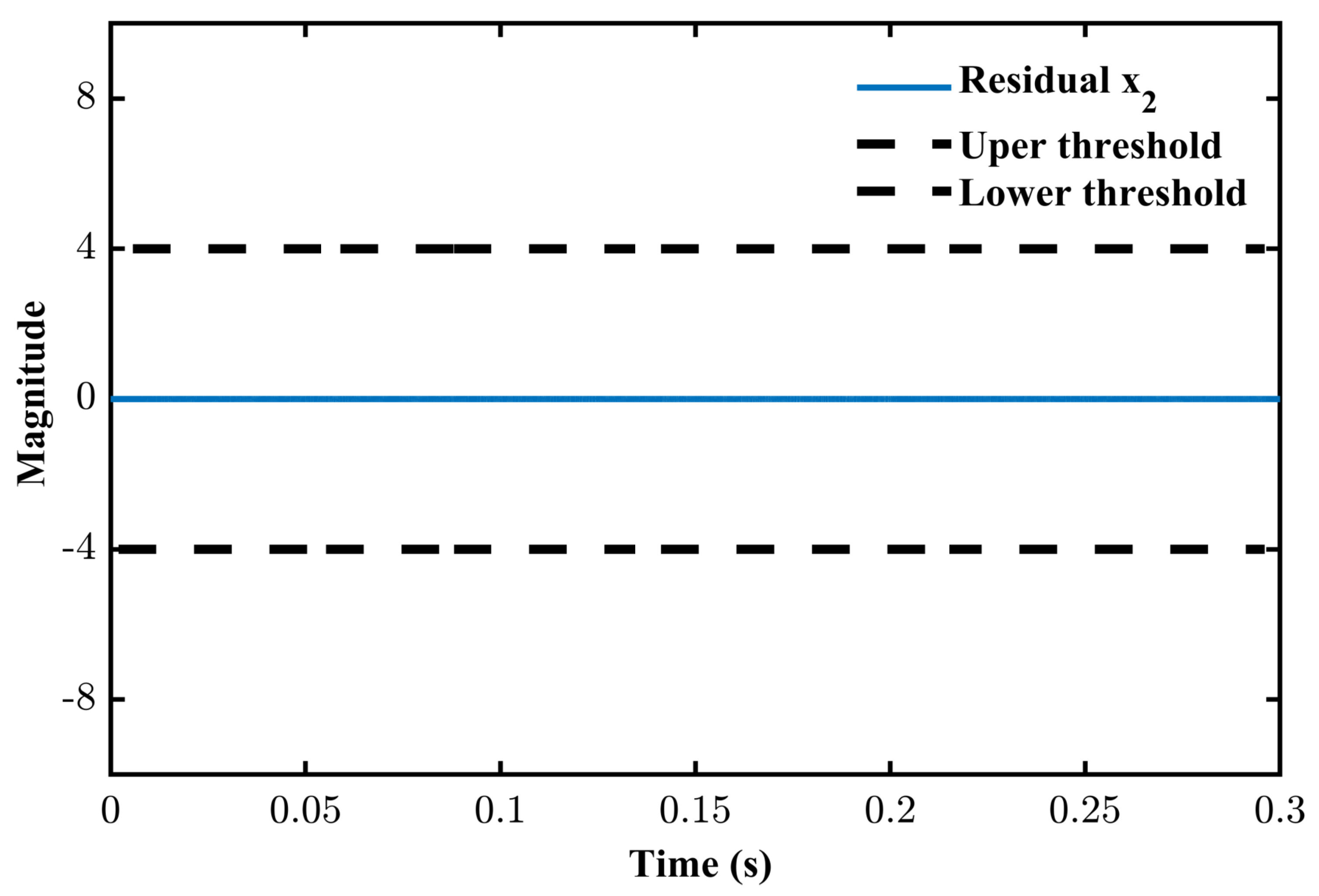
4.2. Residual Construction

The signal, giving an indication of a healthy or faulty system, in FD applications is termed as residual. It is the difference between observer and plant output, usually termed as error signal. The FD is performed on the basis of residual construction.
Let e 1 , e 2 , and e 3 represent the difference between estimated and actual PV array output voltage, inductor current, and output capacitor voltage, respectively. Then, the error dynamics are defined for the three states as follows.
e ˙ 1 = x ˙ ^ 1 x ˙ 1
e ˙ 2 = x ˙ ^ 2 x ˙ 2
e ˙ 3 = x ˙ ^ 3 x ˙ 3
Using Equations (5)–(7) and (12)–(14), the error dynamics in Equations (15)–(17) are transformed as follows.
e ˙ 1 = u ξ 1 C i K 01 ξ 1 K 1 sign ( ξ 1 )
e ˙ 2 = ξ 3 L + u ( ξ 1 + ξ 3 ) L K 02 ξ 2 K 2 sign ( ξ 2 )
e ˙ 3 = ξ 2 L ξ 3 R C 0 u ξ 2 C 0 K 03 ξ 3 K 3 sign ( ξ 3 )
Proposition 1. 
If the gains of the controller ( K 0 i and K i , i = 1 , 2 , 3 ) are positive and large enough, then the error dynamics governed by Equations (18)–(20) converge exponentially.
Proof. 
In order to carry out the stability analysis, Lyapunov function candidates are utilized. Let V 1 be the Lyanpunov function candidate for Equation (18), as this state does not depend upon the other states, so
V 1 = 1 2 e 1 2
Then the total time derivative of Equation (21) along the trajectories of Equation (18) is given by
V ˙ 1 = u e 1 2 C i K 01 e 1 2 K 1 | e 1 |
which is negative definite if K 01 is large enough. This guarantees that e 1 0 exponentially. Now, let V 2 be the Lyapunov function candidate for the other two states such that
V 2 = 1 2 e 2 2 + e 3 2
and
V ˙ 2 = K 02 e 2 2 + K 03 e 3 2 + e 3 2 R C 0 + K 2 | e 2 | + K 3 | e 3 | + u e 2 e 3 1 L 1 C 0
which is also negative definite. Hence, e 2 0 and e 3 0 . This confirms the stability of the proposed SMO. □
It is always appealing to have more options for fetching the real-time information about the system, e.g., having sensors for each and every state. However, adding more components also carries demerits, such as that the system will be bulky, expensive, and prone to more faults/errors.
The proposed SMO is also used to fulfill the purpose of analytical redundancy for estimating the state x 2 using the system information carried with x 1 . From Equations (12)–(14), x 2 is estimated as follows.
x ^ 2 = I p v u x ˙ ^ 1 u K 01 ξ 1 K 1 sign ( ξ 1 )
Specific fault limits are essential for the residual in the FD applications, which is explained in the upcoming section.

4.3. Threshold Design

The residual of the observer signal is zero for a healthy system; however, if there are faults, then a threshold may be defined as one of the two types available, i.e., fixed and dynamic. In the case of fixed thresholds, the fault sensitivity becomes less pronounced, especially when incipient faults occur. In the case of dynamic thresholds, the sensitivity becomes more pronounced, hence facilitating and improving the efficacy of fault diagnosis. Thus, a dynamic threshold function K t h is designed.
e K t h f a = 0 e K t h f a 0
where K t h is the tolerance value and f a is the fault. The forthcoming section is regarding the estimation of x 2 through SMO.

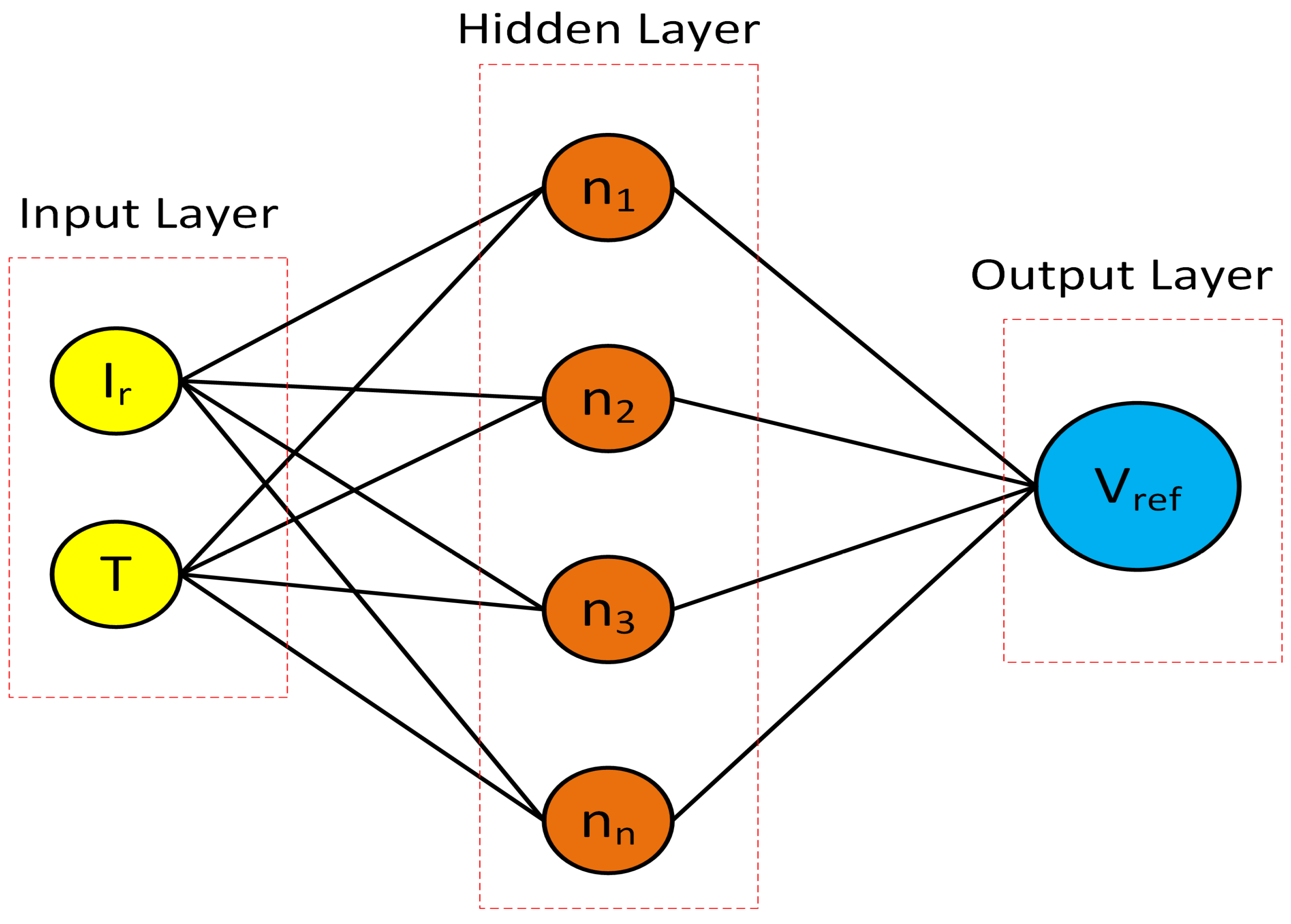
5. Formation of Reference Voltage

A stochastic nature of the environmental inputs to the PV system causes a variation in possible/allowable maximum power point (MPP). Thus, a reference voltage ( V r e f or V p v r ), showing maximum power point tracking (MPPT) under varying environmental conditions, is required. Tracking such reference, with the proposed scheme, will ensure MPPT at the PV system output. A three-layer neural network (NN), trained with different values of irradiance (650–1000 W/m 2 ) and temperature (25–65 °C), is employed to generate the required V r e f .
Let W i j be the weight of the i t h node and j t h neuron of a layer, p i be the input information at an i t h input node, and ( b j o ) be the reconstruction error or bias; then, a net activation of the input layer is computed as follows.
a j = i = 1 n W i j p i + b j o
where j = 1 , 2 , 3 , l o represent the number of neurons in hidden layer. The hidden layer takes a j to generate its i t h output as follows.
y i = f ( a j )
where f ( . ) = T a n h ( . ) is the activation function. Now, let ω k j represent weight between the k t h output layer node and the j t h hidden layer node; then, the net activation of the output layer is as follows.
a k = j = 1 I o ω k j y i + b k o
where k = 1 represents the number of neurons in the output layer. The V r e f is generated at the output layer as a function of its net activation.
V r e f = f ( a k )
A 3D view of the estimated V r e f is shown in Figure 4, while the architecture of the NN is shown in Figure 5, where irradiance I r and temperature T form the input layer, followed by a hidden layer, and then an output layer.

6. Simulation Results

The efficacy of the proposed sliding mode observer (SMO)-based fault diagnosis (FD) scheme is portrayed via simulations in the MATLAB/Simulink environment. As mentioned earlier, the SMO is designed to fulfill two objectives, i.e., FD and estimation of state x 2 .
In the first case, the simulations are performed in the presence of multiple sensor faults and varying environmental conditions (Figure 6) as well as load (Figure 7) to validate the performance of the proposed scheme. Moreover, to extract maximum power from the PV panel and to track the desired reference voltage, a back-stepping controller (BSC) [34] was employed. In addition, the results, for ensuring MPPT, are compared for a BSC alone and a BSC based on the proposed SMO.
The system parameters are shown in Table 1, while parameters of the SMO are listed in Table 2.

6.1. Performance under Varying Conditions in the Presence of Sensor Fault

The robust performance validation of the proposed scheme is carried out by introducing faults, mathematically represented as 6 Sin ( x 1 ) + 0.5 Sin ( x 1 t ) and 8 Sin ( x 1 ) + 1.5 Sin ( x 1 t ) , to the sensor x 1 at the time interval t = [ 0.14 to 0.18 ] and t = [ 0.25 to 0.27 ] ( s ) , respectively. Inherently, at the instances of fault, the maximum power point tracking (MPPT) capability of the PV system is compromised. The proposed scheme copes with this deterioration of MPPT.
As mentioned earlier, the neural network takes the environmental conditions (temperature and irradiance) as input and generates a peak voltage curve. This trajectory/curve serves as a reference for the MPPT algorithm. Thus, following such trajectory ( V r e f ), generated by the neural network, ensures the MPPT.
The PV array output voltage trajectories, attained by a BSC and the SMO-based BSC, are shown in Figure 8. It may be noticed that both schemes effectively track the reference voltage and, hence, attain MPPT. However, in the zoomed portions, a definite degradation in performance is evident in the case of the BSC, at the instances of fault occurrences. The degradation is revealed in the form of significant oscillations about the reference trajectory and, hence, steady-state error. Therefore, the SMO-based BSC is coined to have stamped qualitative transcendence over the BSC.
The subsequent figures (Figure 9 and Figure 10) are the sensing/estimated values of inductive current and capacitive output voltage, respectively. It may be observed that the SMO successfully keeps tracking the trajectories ( x 2 and x 3 ). Furthermore, the deviation from V r e f , at the instances of faults (see Figure 8), is propagated to the other states as well (see zoomed portions in Figure 9 and Figure 10). However, the robustness properties of SMO coped with this variation up to almost 100% effect (see Figure 11).
The core objective of any FD system is to give an indication of the abnormal operation/malfunctioning of the system under consideration. The indication is then used to take prompt actions so that any inconvenience with respect to human and system safety may be avoided. Here, this objective is fulfilled with the introduction of specific thresholds and fault residuals.
Figure 11, Figure 12, and Figure 13 show the residuals for states x 1 , x 2 , and x 3 , respectively. It is revealed that the residual for x 1 crosses the threshold at the instances of faults (see Figure 11), while the residuals for other states remain within the limits. This gives an indication of fault in the sensor for x 1 , and hence it is concluded that the fault has been diagnosed. Moreover, the effect of this fault in only one sensor does not cause much inconvenience in other states, as the residuals are well under the threshold limits.
In addition, the power output from the PV array may also be observed in Figure 14. It is evident that the BSC, in combination with the proposed SMO, achieves the MPPT with negligible distortion caused by the occurring fault.

6.2. Sensorless PV System

The robust nature of the proposed SMO, as coined in the earlier sections, is utilized to introduce analytical redundancy (AR) in the overall PV system. Here, the SMO is employed to estimate the state x 2 using the information from x 1 . Thus, the need for having a sensor for x 2 is nullified, causing cost reduction and fewer maintenance hazards. The estimate, shown in Figure 15, reveals the robustness and accuracy of the SMO.

7. Conclusions

A fast and robust Fault Diagnosis (FD) scheme was the aim of this article for sensor faults in a PV system. An FD scheme based on Sliding Mode Observer (SMO), known for remarkable robustness and parameter invariance, was presented. The FD scheme effectively generated fault residuals, while fault alarms were efficiently initiated by comparing residuals with specific thresholds. In combination with the objective of FD, the SMO served as an Analytical Redundancy (AR) by providing the information/trajectory of the inductor current.
In addition, a Neural Network (NN), taking varying environmental conditions (temperature and irradiance) and resistive load as inputs, was employed to generate reference peak voltage and power trajectories. Thus, the Maximum Power Point Tracking (MPPT) of power output from the PV array was ensured by tracking these reference trajectories.
The probable future research directions/recommendations may include generation of adaptive thresholds for varying faults and an extension to Fault-Tolerant Control (FTC). Moreover, an experimental validation of the proposed FD scheme is also a pronounced future direction.

Author Contributions

Z.A.: investigation, methodology. M.A.K.: methodology, software analysis. Z.A.K.: formal analysis, visualization. W.A.: conceptualization, software analysis, visualization. I.K.: visualization, writing—review and editing, proofreading of technical aspects, mathematical analysis. Q.K.: supervision, validation. M.I.: visualization, formal analysis, methodology, funding acquisition, resources. G.N.: visualization, formal analysis, methodology, funding acquisition, resources. All authors have read and agreed to the published version of the manuscript.

Funding

This research was funded by the Faculty of Electrical and Computer Engineering, Cracow University of Technology and the Ministry of Science and Higher Education, Republic of Poland (grant no. E-1/2023).

Data Availability Statement

No extra data to mention. All the data items are mentioned in the figures.

Acknowledgments

The authors acknowledge the support from the Deanship of Scientific Research, Najran University, Kingdom of Saudi Arabia and the Faculty of Electrical and Computer Engineering, Cracow University of Technology, Republic of Poland. The authors also acknowledge technical support from the Electrical Engineering Department of the COMSATS University Abbotabad Campus, Electrical Engineering Department of the University of Sargodha, Center for Advanced Studies in Telecommunication (CAST @COMSATS University Islamabad), and University of Engineering and Technology, Peshawar, Abbotabad Campus.

Conflicts of Interest

The authors declare no conflict of interest.

Nomenclature

PVPhotovoltaic
SMOSliding mode observer
MPTMaximum power transfer
SDGsStrategic Development Goals
ARAnalytical redundancy
STASuper-twisting algorithm
MPPTMaximum power point tracking
FDFault diagnosis
FTCFault-tolerant control
BSCBack-stepping controller
MRMaterial redundancy
HOSMHigher-order sliding mode
BBCBuck–boost converter

References

  1. Panwar, N.; Kaushik, S.; Kothari, S. Role of renewable energy sources in environmental protection: A review. Renew. Sustain. Energy Rev. 2011, 15, 1513–1524. [Google Scholar] [CrossRef]
  2. Khan, M.A.; Khan, Q.; Khan, L.; Khan, I.; Alahmadi, A.A.; Ullah, N. Robust Differentiator-Based NeuroFuzzy Sliding Mode Control Strategies for PMSG-WECS. Energies 2022, 15, 7039. [Google Scholar] [CrossRef]
  3. Zhao, Y.; Ball, R.; Mosesian, J.; de Palma, J.F.; Lehman, B. Graph-based semi-supervised learning for fault detection and classification in solar photovoltaic arrays. IEEE Trans. Power Electron. 2014, 30, 2848–2858. [Google Scholar] [CrossRef]
  4. Alam, Z.; Khan, L.; Khan, Q.; Ullah, S.; Ahmed, S.; Khan, M.A. Integrated Fault-Diagnoses and Fault-Tolerant MPPT Control Scheme for a Photovoltaic System. In Proceedings of the 2019 15th International Conference on Emerging Technologies (ICET), Peshawar, Pakistan, 2–3 December 2019; pp. 1–6. [Google Scholar] [CrossRef]
  5. Garoudja, E.; Harrou, F.; Sun, Y.; Kara, K.; Chouder, A.; Silvestre, S. Statistical fault detection in photovoltaic systems. Sol. Energy 2017, 150, 485–499. [Google Scholar] [CrossRef]
  6. Davarifar, M.; Rabhi, A.; El Hajjaji, A. Comprehensive modulation and classification of faults and analysis their effect in DC side of photovoltaic system. Energy Power Eng. 2013, 5, 230. [Google Scholar] [CrossRef]
  7. Balfour, J.R.; Shaw, M. Introduction to Photovoltaic System Design; Jones & Bartlett Publishers: Sudbury, MA, USA, 2011; ISBN 9781449624682. [Google Scholar]
  8. Jamil, M.; Rizwan, M.; Kothari, D.P. Grid Integration of Solar Photovoltaic Systems; CRC Press: Boca Raton, FL, USA, 2017; ISBN 9781315156347. [Google Scholar] [CrossRef]
  9. Pillai, D.S.; Rajasekar, N. A comprehensive review on protection challenges and fault diagnosis in PV systems. Renew. Sustain. Energy Rev. 2018, 91, 18–40. [Google Scholar] [CrossRef]
  10. Mellit, A.; Tina, G.M.; Kalogirou, S.A. Fault detection and diagnosis methods for photovoltaic systems: A review. Renew. Sustain. Energy Rev. 2018, 91, 1–17. [Google Scholar] [CrossRef]
  11. Madeti, S.R.; Singh, S. A comprehensive study on different types of faults and detection techniques for solar photovoltaic system. Sol. Energy 2017, 158, 161–185. [Google Scholar] [CrossRef]
  12. Wang, Z.; Chen, J.; Cheng, M.; Zheng, Y. Fault-tolerant control of paralleled-voltage-source-inverter-fed PMSM drives. IEEE Trans. Ind. Electron. 2015, 62, 4749–4760. [Google Scholar] [CrossRef]
  13. Salehifar, M.; Arashloo, R.S.; Moreno-Equilaz, J.M.; Sala, V.; Romeral, L. Fault detection and fault tolerant operation of a five phase PM motor drive using adaptive model identification approach. IEEE J. Emerg. Sel. Top. Power Electron. 2013, 2, 212–223. [Google Scholar] [CrossRef]
  14. Berriri, H.; Naouar, M.W.; Slama-Belkhodja, I. Easy and fast sensor fault detection and isolation algorithm for electrical drives. IEEE Trans. Power Electron. 2011, 27, 490–499. [Google Scholar] [CrossRef]
  15. Varrier, S.; Koenig, D.; Martinez, J.J. A parity space-based fault detection on lpv systems: Approach for vehicle lateral dynamics control system. IFAC Proc. Vol. 2012, 45, 1191–1196. [Google Scholar] [CrossRef]
  16. Frank, P.M.; Ding, X. Survey of robust residual generation and evaluation methods in observer-based fault detection systems. J. Process. Control 1997, 7, 403–424. [Google Scholar] [CrossRef]
  17. Kinnaert, M. Robust fault detection based on observers for bilinear systems. Automatica 1999, 35, 1829–1842. [Google Scholar] [CrossRef]
  18. Shields, D. Observer-based residual generation for fault diagnosis for non-affine non-linear polynomial systems. Int. J. Control 2005, 78, 363–384. [Google Scholar] [CrossRef]
  19. Campos-Delgado, D.U.; Espinoza-Trejo, D.R. An observer-based diagnosis scheme for single and simultaneous open-switch faults in induction motor drives. IEEE Trans. Ind. Electron. 2010, 58, 671–679. [Google Scholar] [CrossRef]
  20. Jiang, W.; Dong, C.; Niu, E.; Wang, Q. Observer-based robust fault detection filter design and optimization for networked control systems. Math. Probl. Eng. 2015, 2015, 231749. [Google Scholar] [CrossRef] [Green Version]
  21. Poon, J.; Jain, P.; Konstantakopoulos, I.C.; Spanos, C.; Panda, S.K.; Sanders, S.R. Model-based fault detection and identification for switching power converters. IEEE Trans. Power Electron. 2016, 32, 1419–1430. [Google Scholar] [CrossRef]
  22. Rehman, A.U.; Khan, L.; Ali, N.; Alam, Z.; Khan, Z.A.; Khan, M.A. Soft Computing Technique based Nonlinear Sliding Mode Control for Stand-Alone Photovoltaic System. In Proceedings of the 2020 International Conference on Emerging Trends in Smart Technologies (ICETST), Karachi, Pakistan, 26–27 March 2020; pp. 1–6. [Google Scholar] [CrossRef]
  23. Zorgani, Y.A.; Koubaa, Y.; Boussak, M. MRAS state estimator for speed sensorless ISFOC induction motor drives with Luenberger load torque estimation. ISA Trans. 2016, 61, 308–317. [Google Scholar] [CrossRef]
  24. Tabbache, B.; Benbouzid, M.E.H.; Kheloui, A.; Bourgeot, J.M. Virtual-sensor-based maximum-likelihood voting approach for fault-tolerant control of electric vehicle powertrains. IEEE Trans. Veh. Technol. 2012, 62, 1075–1083. [Google Scholar] [CrossRef] [Green Version]
  25. Khan, M.A.; Ullah, S.; Khan, L.; Khan, Q.; Khan, Z.A.; Zaman, H.; Ahmad, S. Observer Based Higher Order Sliding Mode Control Scheme for PMSG-WECS. In Proceedings of the 2019 15th International Conference on Emerging Technologies (ICET), Peshawar, Pakistan, 2–3 December 2019; pp. 1–6. [Google Scholar] [CrossRef]
  26. Khan, R.; Khan, L.; Ullah, S.; Sami, I.; Ro, J.S. Backstepping based super-twisting sliding mode MPPT control with differential flatness oriented observer design for photovoltaic system. Electronics 2020, 9, 1543. [Google Scholar] [CrossRef]
  27. Luenberger, D. An introduction to observers. IEEE Trans. Autom. Control 1971, 16, 596–602. [Google Scholar] [CrossRef]
  28. Afri, C.; Andrieu, V.; Bako, L.; Dufour, P. State and parameter estimation: A nonlinear Luenberger observer approach. IEEE Trans. Autom. Control 2016, 62, 973–980. [Google Scholar] [CrossRef] [Green Version]
  29. Apaza-Perez, W.A.; Moreno, J.A.; Fridman, L.M. Dissipative approach to sliding mode observers design for uncertain mechanical systems. Automatica 2018, 87, 330–336. [Google Scholar] [CrossRef]
  30. Iqbal, M.; Bhatti, A.I.; Ayubi, S.I.; Khan, Q. Robust parameter estimation of nonlinear systems using sliding-mode differentiator observer. IEEE Trans. Ind. Electron. 2010, 58, 680–689. [Google Scholar] [CrossRef]
  31. Park, H.; Kim, H. PV cell modeling on single-diode equivalent circuit. In Proceedings of the IECON 2013—39th Annual Conference of the IEEE Industrial Electronics Society, Vienna, Austria, 10–13 November 2013; pp. 1845–1849. [Google Scholar] [CrossRef]
  32. Yaqoob, S.J.; Motahhir, S.; Agyekum, E.B. A new model for a photovoltaic panel using Proteus software tool under arbitrary environmental conditions. J. Clean. Prod. 2022, 333, 130074. [Google Scholar] [CrossRef]
  33. Yaqoob, S.J.; Saleh, A.L.; Motahhir, S.; Agyekum, E.B.; Nayyar, A.; Qureshi, B. Comparative study with practical validation of photovoltaic monocrystalline module for single and double diode models. Sci. Rep. 2021, 11, 19153. [Google Scholar] [CrossRef]
  34. Armghan, H.; Ahmad, I.; Armghan, A.; Khan, S.; Arsalan, M. Backstepping based non-linear control for maximum power point tracking in photovoltaic system. Sol. Energy 2018, 159, 134–141. [Google Scholar] [CrossRef]
Figure 1. Single-diode model of PV cell.
Electronics 12 00282 g001
Figure 2. A complete PV model with a variable resistive load and an observer.
Electronics 12 00282 g002
Figure 3. FD scheme using SMO.
Electronics 12 00282 g003
Figure 4. 3D plot of reference voltage.
Electronics 12 00282 g004
Figure 5. Internal architecture of NN.
Electronics 12 00282 g005
Figure 6. Varying temperature and irradiance profile.
Electronics 12 00282 g006
Figure 7. Varying resistive load profile.
Electronics 12 00282 g007
Figure 8. Fault effect on sensor x 1 .
Electronics 12 00282 g008
Figure 9. Fault effect on sensor x 2 .
Electronics 12 00282 g009
Figure 10. Fault effect on sensor x 3 .
Electronics 12 00282 g010
Figure 11. Residual formation of sensor x 1 .
Electronics 12 00282 g011
Figure 12. Residual formation of sensor x 2 .
Electronics 12 00282 g012
Figure 13. Residual formation of sensor x 3 .
Electronics 12 00282 g013
Figure 14. MPPT by the proposed SMO and BSC.
Electronics 12 00282 g014
Figure 15. Estimated state by SMO.
Electronics 12 00282 g015
Table 1. PV array parameters [34].
ParametersSymbolValue
Total modules in PV array N m 16
Number of modules connected in series N s 4
Number of modules connected in parallel N p 4
Number of cells per modules N c 72
Voltage at open circuit V o c 165.8 V
Current at short circuit I s c 17.56 A
Voltage at maximum power V m p p 102.6 V
Current at maximum power I m p p 15.16 A
Maximum power P m a x 1555.4 W
Input capacitor C i 1 × 10 3 F
InductorL 20 × 10 3 H
Table 2. SMO parameters.
S.NO.SymbolValue
1 K 1 100
2 K 2 9000
3 K 3 10
4 K 01 10
5 K 02 10
6 K 03 10
Disclaimer/Publisher’s Note: The statements, opinions and data contained in all publications are solely those of the individual author(s) and contributor(s) and not of MDPI and/or the editor(s). MDPI and/or the editor(s) disclaim responsibility for any injury to people or property resulting from any ideas, methods, instructions or products referred to in the content.

