
A Method for Calculating the Derivative of Activation Functions Based on Piecewise Linear Approximation

Abstract
:1. Introduction
- We use least squares to improve a general, error-controlled PWL approximation method to obtain fewer segments or smaller average errors, and then extend it to the calculation of various activation functions and their derivatives.
- We evaluate the applicability of the method in neural networks in terms of convergence speed, generalization ability, and hardware overhead.
- We replace the derivative calculation in the neural network training task with proposed method and verified its effectiveness on a three-layer perceptron: our method reduced the backpropagation computation time by 4–6% with the same or even slightly higher classification accuracy.
2. Methods
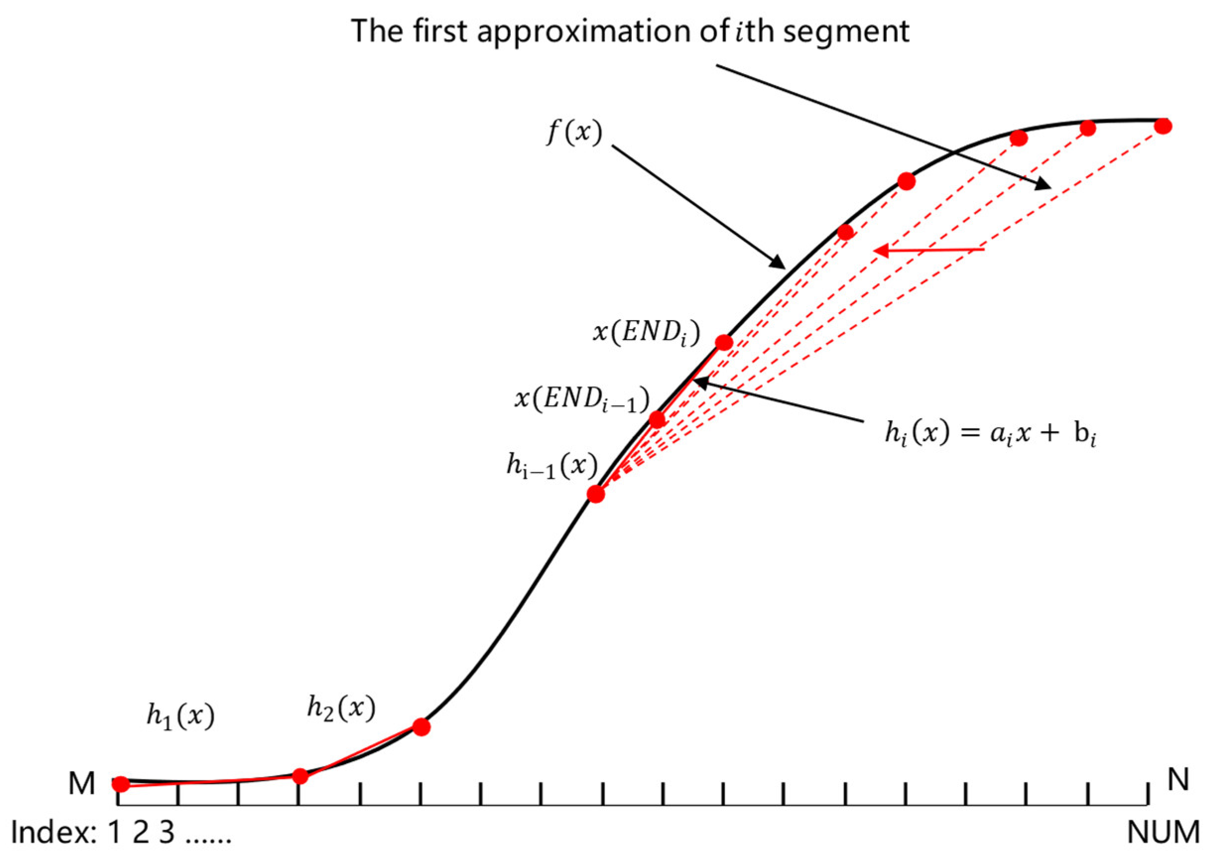
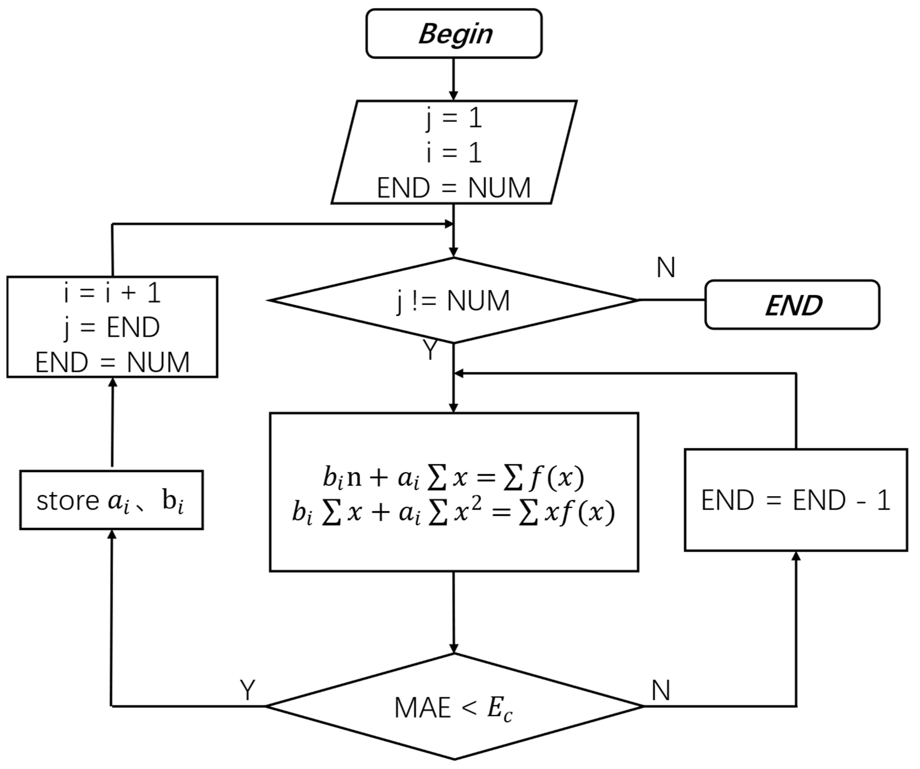
2.1. PWLMMAE
2.1.1. Input Range Discretization
2.1.2. Minimization of MAE for a Given Width of Subinterval
2.1.3. Segmentation Points
2.2. PWL Approximation to Derivatives
3. Experiment
3.1. Experimental Setup
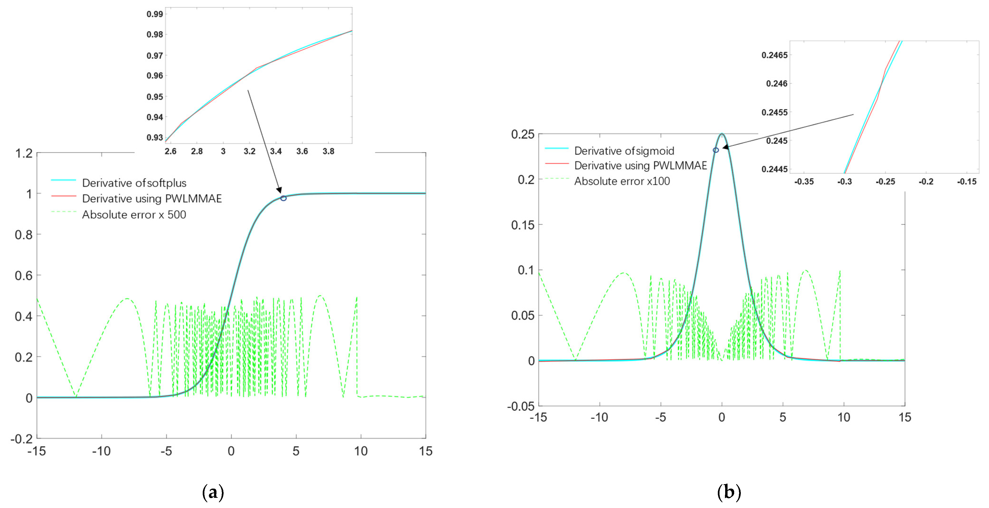
3.2. Segment Approximation Comparison
3.3. Evaluate PWLMMAE
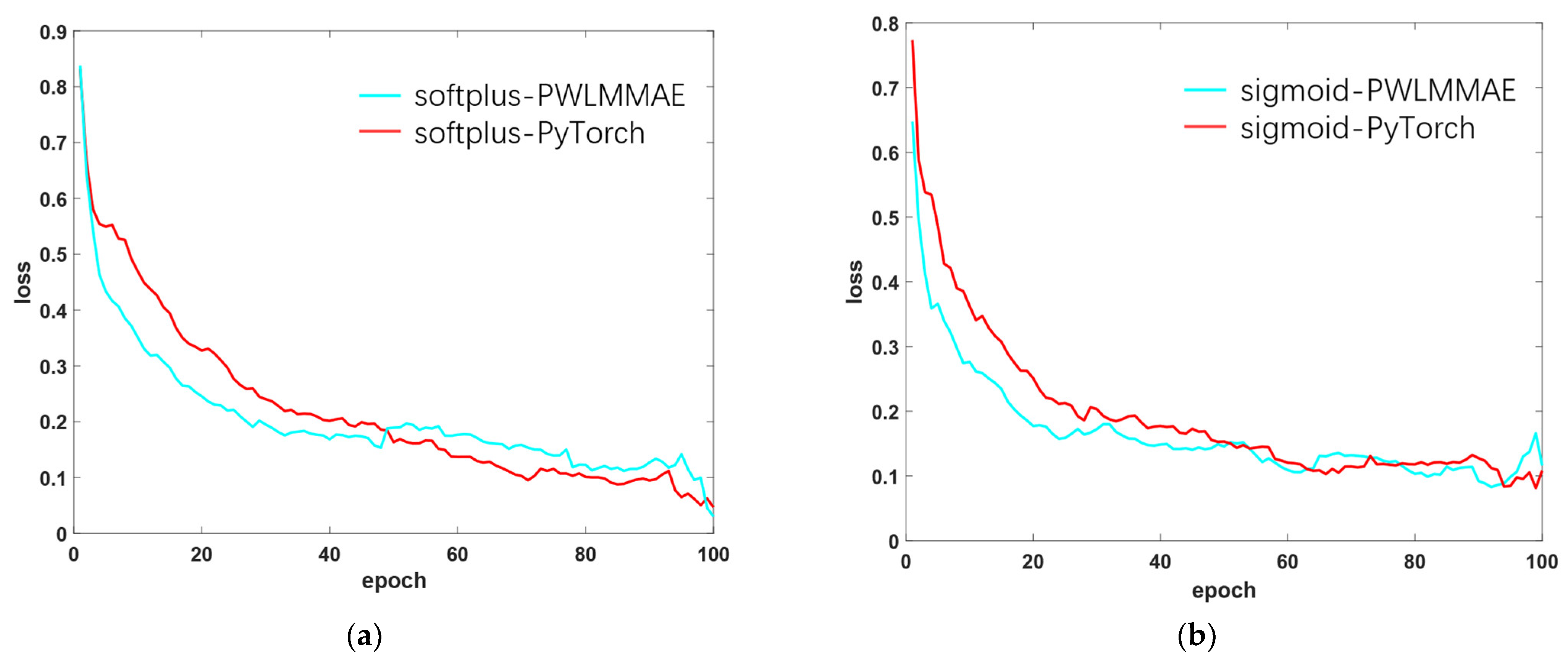
3.3.1. Speed of Convergence
3.3.2. Capability of Generalization
3.3.3. Hardware Overhead and Speed
3.4. Performance Comparisons
4. Conclusions
Author Contributions
Funding
Data Availability Statement
Conflicts of Interest
References
- Liu, Z.; Dou, Y.; Jiang, J.; Xu, J.; Li, S.; Zhou, Y.; Xu, Y. Throughput-Optimized FPGA Accelerator for Deep Convolutional Neural Networks. ACM Trans. Reconfig. Technol. Syst. 2017, 10, 1–23. [Google Scholar] [CrossRef]
- Qiao, Y.; Shen, J.; Xiao, T.; Yang, Q.; Wen, M.; Zhang, C. FPGA-Accelerated Deep Convolutional Neural Networks for High Throughput and Energy Efficiency. Concurr. Computat. Pract. Exper. 2017, 29, e3850. [Google Scholar] [CrossRef]
- Yu, Y.; Wu, C.; Zhao, T.; Wang, K.; He, L. OPU: An FPGA-Based Overlay Processor for Convolutional Neural Networks. IEEE Trans. VLSI Syst. 2020, 28, 35–47. [Google Scholar] [CrossRef]
- Li, B.; Pandey, S.; Fang, H.; Lyv, Y.; Li, J.; Chen, J.; Xie, M.; Wan, L.; Liu, H.; Ding, C. FTRANS: Energy-Efficient Acceleration of Transformers Using FPGA. In Proceedings of the ACM/IEEE International Symposium on Low Power Electronics and Design, Boston, MA, USA, 10–12 August 2020. [Google Scholar]
- Lu, S.; Wang, M.; Liang, S.; Lin, J.; Wang, Z. Hardware Accelerator for Multi-Head Attention and Position-Wise Feed-Forward in the Transformer. In Proceedings of the 2020 IEEE 33rd International System-on-Chip Conference (SOCC), Las Vegas, NV, USA, 8–11 September 2020. [Google Scholar]
- Khan, H.; Khan, A.; Khan, Z.; Huang, L.B.; Wang, K.; He, L. NPE: An FPGA-Based Overlay Processor for Natural Language Processing. In Proceedings of the 2021 ACM/SIGDA International Symposium on Field-Programmable Gate Arrays, Monterey, CA, USA, 28 February–2 March 2021. [Google Scholar]
- Zhao, W.; Fu, H.; Luk, W.; Yu, T.; Wang, S.; Feng, B.; Ma, Y.; Yang, G. F-CNN: An FPGA-Based Framework for Training Convolutional Neural Networks. In Proceedings of the 2016 IEEE 27th International Conference on Application-specific Systems, Architectures and Processors (ASAP), London, UK, 6–8 July 2016. [Google Scholar]
- Liu, Z.; Dou, Y.; Jiang, J.; Wang, Q.; Chow, P. An FPGA-Based Processor for Training Convolutional Neural Networks. In Proceedings of the 2017 International Conference on Field Programmable Technology (ICFPT), Melbourne, VIC, Australia, 11–13 December 2017. [Google Scholar]
- Ramachandran, P.; Zoph, B.; Le, Q.V. Swish: A Self-Gated Activation Function. arXiv 2017, arXiv:1710.05941v1. [Google Scholar]
- Dugas, C.; Bengio, Y.; Bélisle, F.; Nadeau, C.; Garcia, R. Incorporating Second-Order Functional Knowledge for Better Option Pricing. In Proceedings of the 13th International Conference on Neural Information Processing Systems, Denver, CO, USA, 1 January 2000. [Google Scholar]
- Rumelhart, D.E.; Hinton, G.E.; Williams, R.J. Learning representations by back propagating errors. Nature 1986, 323, 533–536. [Google Scholar] [CrossRef]
- Baydin, A.G.; Pearlmutter, B.A.; Radul, A.A.; Siskind, J.M. Automatic Differentiation in Machine Learning: A Survey. J. Mach. Learn. Res. 2015, 18, 153:1–153:43. [Google Scholar]
- Frenzen, C.L.; Sasao, T.; Butler, J.T. On the Number of Segments Needed in a Piecewise Linear Approximation. J. Comput. Appl. Math. 2010, 234, 437–446. [Google Scholar] [CrossRef] [Green Version]
- Gutierrez, R.; Valls, J. Low Cost Hardware Implementation of Logarithm Approximation. IEEE Trans. VLSI Syst. 2011, 19, 2326–2330. [Google Scholar] [CrossRef]
- Kim, H.; Nam, B.-G.; Sohn, J.-H.; Woo, J.-H.; Yoo, H.-J. A 231-MHz, 2.18-MW 32-Bit Logarithmic Arithmetic Unit for Fixed-Point 3-D Graphics System. IEEE J. Solid-State Circuits 2006, 41, 2373–2381. [Google Scholar] [CrossRef] [Green Version]
- Berjón, D.; Gallego, G.; Cuevas, C.; Morán, F.; García, N. Optimal Piecewise Linear Function Approximation for GPU-Based Applications. IEEE Trans. Cybern. 2016, 46, 2584–2595. [Google Scholar] [CrossRef] [Green Version]
- Chiluveru, S.R.; Tripathy, M.; Chunarkar, S. A Controlled Accuracy-Based Recursive Algorithm for Approximation of Sigmoid Activation. Natl. Acad. Sci. Lett. 2021, 44, 541–544. [Google Scholar] [CrossRef]
- Sun, H.; Luo, Y.; Ha, Y.; Shi, Y.; Gao, Y.; Shen, Q.; Pan, H. A Universal Method of Linear Approximation With Controllable Error for the Efficient Implementation of Transcendental Functions. IEEE Trans. Circuits Syst. I 2020, 67, 177–188. [Google Scholar] [CrossRef]
- Srivastava, H.M.; Ansari, K.J.; Özger, F.; Ödemiş Özger, Z. A Link between Approximation Theory and Summability Methods via Four-Dimensional Infinite Matrices. Mathematics 2021, 9, 1895. [Google Scholar] [CrossRef]
- Cai, Q.-B.; Ansari, K.J.; Temizer Ersoy, M.; Özger, F. Statistical Blending-Type Approximation by a Class of Operators That Includes Shape Parameters λ and α. Mathematics 2022, 10, 1149. [Google Scholar] [CrossRef]
- Özger, F.; Aljimi, E.; Temizer Ersoy, M. Rate of Weighted Statistical Convergence for Generalized Blending-Type Bernstein-Kantorovich Operators. Mathematics 2022, 10, 2027. [Google Scholar] [CrossRef]
- Sigillito, V.G.; Wing, S.P.; Hutton, L.V.; Baker, K.B. Classification of radar returns from the ionosphere using neural networks. Johns Hopkins APL Tech. Dig. 1989, 10, 262–266. [Google Scholar]
- Gironés, R.G.; Gironés, R.G.; Palero, R.C.; Boluda, J.C.; Boluda, J.C.; Cortés, A.S. FPGA Implementation of a Pipelined On-Line Backpropagation. J. VLSI Signal Process. Syst. Signal Image Video Technol. 2005, 40, 189–213. [Google Scholar] [CrossRef]
- Horowitz, M. 1.1 Computing’s Energy Problem (and What We Can Do about It). In Proceedings of the 2014 IEEE International Solid-State Circuits Conference Digest of Technical Papers (ISSCC), San Francisco, CA, USA, 20–26 February 2014. [Google Scholar]


| Function | Input_Range | Q | Method | NO. of Segment | ||
|---|---|---|---|---|---|---|
| sigmoid | (−15,15) | 4 | 0.001 | [18] | 4.65 × 10⁻⁴ | 21 |
| This | 3.96 × 10⁻⁴ | 20 | ||||
| 0.0005 | [18] | 2.61 × 10⁻⁴ | 29 | |||
| This | 2.16 × 10⁻⁴ | 29 | ||||
| tanh | (−4,4) | 4 | 0.001 | [18] | 5.00 × 10⁻⁴ | 30 |
| This | 4.94 × 10⁻⁴ | 31 | ||||
| 0.0005 | [18] | 2.39 × 10⁻⁴ | 52 | |||
| This | 2.61 × 10⁻⁴ | 46 |
| Activation Function | Macro-P | Macro-R | Macro-F1 |
|---|---|---|---|
| sigmoid-PyTorch | 0.90195 | 0.82159 | 0.85989 |
| sigmoid-PWLMMAE | 0.90438 | 0.81338 | 0.85647 |
| Activation Function | Macro-P | Macro-R | Macro-F1 |
|---|---|---|---|
| softplus-PyTorch | 0.92694 | 0.79302 | 0.85477 |
| softplus-PWLMMAE | 0.91681 | 0.80705 | 0.85844 |
| Function | Q(Bits) | Acc Average | NO. of Segment | |
|---|---|---|---|---|
| Sigmoid | 2 | 0.25 | 87.27 | 2 |
| 3 | 0.125 | 88.93 | 3 | |
| 4 | 0.0625 | 89.82 | 3 | |
| Softplus | 2 | 0.25 | 90.10 | 2 |
| 3 | 0.125 | 90.01 | 3 | |
| 4 | 0.0625 | 90.19 | 3 |
| Activation Function | Accuracy | Backward Time(s) |
|---|---|---|
| Sigmoid-PyTorch | 90.00 | 2.031 |
| Sigmoid-PWLMMAE | 89.82 | 1.935 |
| Softplus-PyTorch | 89.91 | 2.139 |
| Softplus-PWLMMAE | 90.19 | 2.005 |
Disclaimer/Publisher’s Note: The statements, opinions and data contained in all publications are solely those of the individual author(s) and contributor(s) and not of MDPI and/or the editor(s). MDPI and/or the editor(s) disclaim responsibility for any injury to people or property resulting from any ideas, methods, instructions or products referred to in the content. |
© 2023 by the authors. Licensee MDPI, Basel, Switzerland. This article is an open access article distributed under the terms and conditions of the Creative Commons Attribution (CC BY) license (https://creativecommons.org/licenses/by/4.0/).
Share and Cite
Liao, X.; Zhou, T.; Zhang, L.; Hu, X.; Peng, Y. A Method for Calculating the Derivative of Activation Functions Based on Piecewise Linear Approximation. Electronics 2023, 12, 267. https://doi.org/10.3390/electronics12020267
Liao X, Zhou T, Zhang L, Hu X, Peng Y. A Method for Calculating the Derivative of Activation Functions Based on Piecewise Linear Approximation. Electronics. 2023; 12(2):267. https://doi.org/10.3390/electronics12020267
Chicago/Turabian StyleLiao, Xuan, Tong Zhou, Longlong Zhang, Xiang Hu, and Yuanxi Peng. 2023. "A Method for Calculating the Derivative of Activation Functions Based on Piecewise Linear Approximation" Electronics 12, no. 2: 267. https://doi.org/10.3390/electronics12020267