Anomaly-PTG: A Time Series Data-Anomaly-Detection Transformer Framework in Multiple Scenarios

Abstract

In actual scenarios, industrial and cloud computing platforms usually need to monitor equipment and traffic anomalies through multivariable time series data. However, the existing anomaly detection methods can not capture the long-distance temporal correlations of data and the potential relationships between features simultaneously, and only have high detection accuracy for specific time sequence anomaly detection scenarios without good generalization ability. This paper proposes a time-series anomaly-detection framework for multiple scenarios, Anomaly-PTG (anomaly parallel transformer GRU), given the above limitations. The model uses the parallel transformer GRU as the information extraction module of the model to learn the long-distance correlation between timestamps and the global feature relationship of multivariate time series, which enhances the ability to extract hidden information from time series data. After extracting the information, the model learns the sequential representation of the data, conducts the sequential modeling, and transmits the data to the full connection layer for prediction. At the same time, it also uses the autoencoder to learn the potential representation of the data and reconstruct the data. The two are optimally combined to form an anomaly detection module of the model. The module combines timestamp prediction with time series data reconstruction, improving the detection rate of rare anomalies and detection accuracy. By using three public datasets of physical devices and one dataset of network traffic intrusion detection, the model’s effectiveness was verified, and the model’s generalization ability and strong robustness were demonstrated. Compared with the most advanced method, the average F1 value of the Anomaly-PTG model on four datasets was increased by 2.2%, and the F1 value on each dataset was over 94%.

1. Introduction

At present, multivariable-time-series anomaly detection embraces broad applications in the industry [1,2], network security [3], the Internet of Things [4,5,6], aerospace, and other fields [7]. By monitoring time series data, it can avoid resource loss and security risks caused by equipment failures and network attacks. Anomaly detection of time series data comprises univariate-time-series anomaly detection and multivariable-time-series anomaly detection. The former only focuses on data anomaly in a single feature dimension. If a single variable does not conform to the overall data distribution, it will be detected as an outlier. The latter is composed of multiple features, including two abnormal detection ways. The first is to infer the possibility of overall anomaly occurrence through the change of a single feature and combine all captured univariate anomalies by calculation means of mean or standard deviation as the evaluation result for multivariable anomaly detection [8,9]. The second method is to extract the correlation information between multiple variables and perform algorithm analysis by learning the global probability distribution of data and then directly give the abnormal detection results.

In recent years, much research based on deep learning has been presented. K Hundman et al. [7] raised an LSTM-based spacecraft method. The autoencoder-based time series method is raised by Salahud et al. [10]. Zhao et al. [11] applied a graph neural network (GNN) to study the correlation among multiple variables in time series. However, there are still three limitations caused by these methods. The first is that they do not capture the long-distance time information well; the second is that they do not pay attention to the connection between features; the third is that some methods only show certain high detection accuracy for specific scenes without excellent generalization ability. Therefore, exploring a high-precision anomaly detection model for a wide range of tasks is essential in this field.

The transformer [12] serves as a very popular structure for deep learning. It is first put forward for NLP tasks such as machine translation because of its excellent performance in capturing remote time information and global representation, and currently, it is extended to machine vision, time series, and other fields. A novel anomaly detection model, anomaly parallel transformer GRU (Anomaly-PTG), is proposed in this paper. It can capture the time correlation of each time point and the potential relationship between each feature through the attention mechanism models the long-distance time information and the global relationship, and learns the extracted timing information through GRU to get a better timing representation. The contributions produced by this paper are listed:

(1) A novel multivariable timing anomaly detection model (Anomaly-PTG) is proposed, which can simultaneously extract feature relations and remote time dependence from time series through a parallel transformer GRU.

(2) A transformer is improved to make it more suitable for extracting information from time series data and more widely used for multivariable-time-series anomaly detection tasks in other scenarios.

(3) The model has been proved by extensive experiments to outperform the current models on three large public datasets and applied to a network intrusion dataset to obtain excellent anomaly detection performance. The average F1 value across the four datasets has improved by 2.2% compared with the most advanced approach currently.

The remaining paper is organized as such: Section 2 refers to related work in the multivariable-time-series anomaly detection. The structure of the Anomaly-PTG model and the required techniques have been introduced in Section 3. Then, Section 4 is the experimental process and experimental results. Section 5 summarizes the full text and future research.

2. Related Works

This section analyzes and studies the current popular time-series anomaly detection algorithms. This paper introduces the multivariate-time-series anomaly detection method and the main techniques used in this paper.

2.1. Multivariable Exception Detection

Multivariable-time-series anomaly detection is always the focus of time-series anomaly detection. In recent years, many deep learning-based methods have achieved good performances—for example, based on a long and short-term memory (LSTM) [13] network, the deep autoencoder Gaussian mixture model (DAGMM) [14], and variational autoencoder (VAE) [15]. These models use prediction-based or reconstruction-based ways to detect anomalies in multivariable time series and are the most popular methods in the field currently.

The representative model based on the prediction method is RNN, which can improve the model’s prediction ability by retaining the observed values of past time points. It is a very suitable structure for modeling time series data. The LSTM-based method is improved based on RNN, and the gating mechanism is adopted to solve the disappearance or explosion gradient problem in RNN training. It is a more commonly used anomaly detection model for time series. These prediction-based models [16] are the basis of anomaly detection by predicting the error between the output at the next moment and the actual observation value. However, the limitation of this method is that the predicted values are often inaccurate or unpredictable, which will lead to a high rate of abnormal missed detection.

In addition, the methods based on reconstruction convert the input multivariable time series to a low-dimensional implicit vector and then reconstruct the low-dimensional vector to generate reconstruction errors to serve as the basis for anomaly detection. For example, DAGMM uses the reconstruction network, and the low-dimensional information representation proceeds with density estimation for reconstruction error reduction.

However, the method cannot capture the feature correlation in time series information, and there are some limitations, such as slow training speed and abnormal omissions. The LSTM-VAE [17] uses LSTM as a low-dimensional embedding of the VAE and captures the sequential patterns. The OmniAnomaly model [18] can obtain the latent space’s probability distribution by combining VAE and GRU [19] and uses techniques of random variable connectivity and plane normalization to catch the normal patterns for multivariable time series.

In reconstruction-based or forecast methods, Hang Zhao et al. [11] and Guan S et al. [20] proved that prediction-based and reconstruction-based methods are complementary. The former proposed the MTAD-GAT model to input the time series data into the model in the form of a graph. The latter comes up with GTAD combines graph attention mechanism and temporal convolution to capture data information in more detail. The graph bias network GDN was prepared by Ailin Deng et al. [21], who regarded each sensor as a node of the graph and obtained the correlation between each sensor to explain the deviation of the learning mode.

The graph neural network can directly obtain the relationship between features and improve the training speed, but it is insufficient to capture the long-range temporal dependence of time series data. At present, adversarial generative networks (GAN) welcome a more extensive scope of application for time-series anomaly detection [22,23]. For example, Dan Li et al. proposed the MAD-GAN [24] model, which is a method to detect multivariable time-series anomalies in an unsupervised way. It will capture the potential interaction information between variables in the whole data and learn the correlation of time series from an overall perspective. Unsupervised anomaly detection methods based on the antagonistic generative network also include USAD proposed by Julien Audibert et al. [25].

In this method, the reconstruction ability of the automatic encoder is continuously improved by means of confrontation training so as to reduce the reconstruction error. However, the limitation of these models is that they do not explicitly learn the relationship between the features and the lack of use of long-distance time information.

2.2. Transformer Models for Time Series

For the last few years, transformers have been employed in a wide variety of professions. The attention mechanism it proposes breaks the limitations of traditional recurrent neural networks. Depending on the advantages of capturing long-distance information, in natural language processing (NLP) [26,27], computer vision and other fields [28,29] have shown strong performance, breaking away from the limitations of the original method and becoming the mainstream deep learning method.

The transformer is a prevalent method in time series prediction [30,31] and anomaly detection [32,33] because its characteristics are very suitable for modeling time series data. For example, the informer [34] prediction model proposed by Haoyi Zhou et al. improves the prediction effect of the model by capturing the long-distance time information of the input and output data through the transformer and improves the traditional transformer structure, reducing the complexity of the model and breaking the limitations of the original structure. The TranAD [35] model proposed by Shreshth Tuli et al. is an anomaly detection method that combines the transformer and meta-learning. The model adopts adaptive and antagonistic training methods so that its architecture can be quickly trained and tested while maintaining the stability of the model.

The GTA [36] model proposed by Chen et al. puts forward a strategy of using connection learning to learn graph structure, which can model the time dependence of the architecture based on the transformer. It is a new framework for anomaly detection of multivariate time series applied in the Internet of Things. The above methods are aimed at improving the structure of the transformer.

In contrast, the anomaly transformer proposed by Jiehui Xu et al. [37] innovatively put forward the anomaly attention mechanism. It used series association and prior association to capture the correlation difference between each time point and defined a new criterion for anomaly discrimination. These methods prove the effectiveness of the transformer in this field. Based on the research and analysis of the above methods, we improved the structure of the transformer and decoded the time-dependent long-distance information and feature relationship captured by the transformer through GRU, which reduced the number of parameters of the model, enhanced the stability of the training model, and did not need to input data to the decoding end. It is a more suitable structure for timing anomaly detection.

3. Methodology

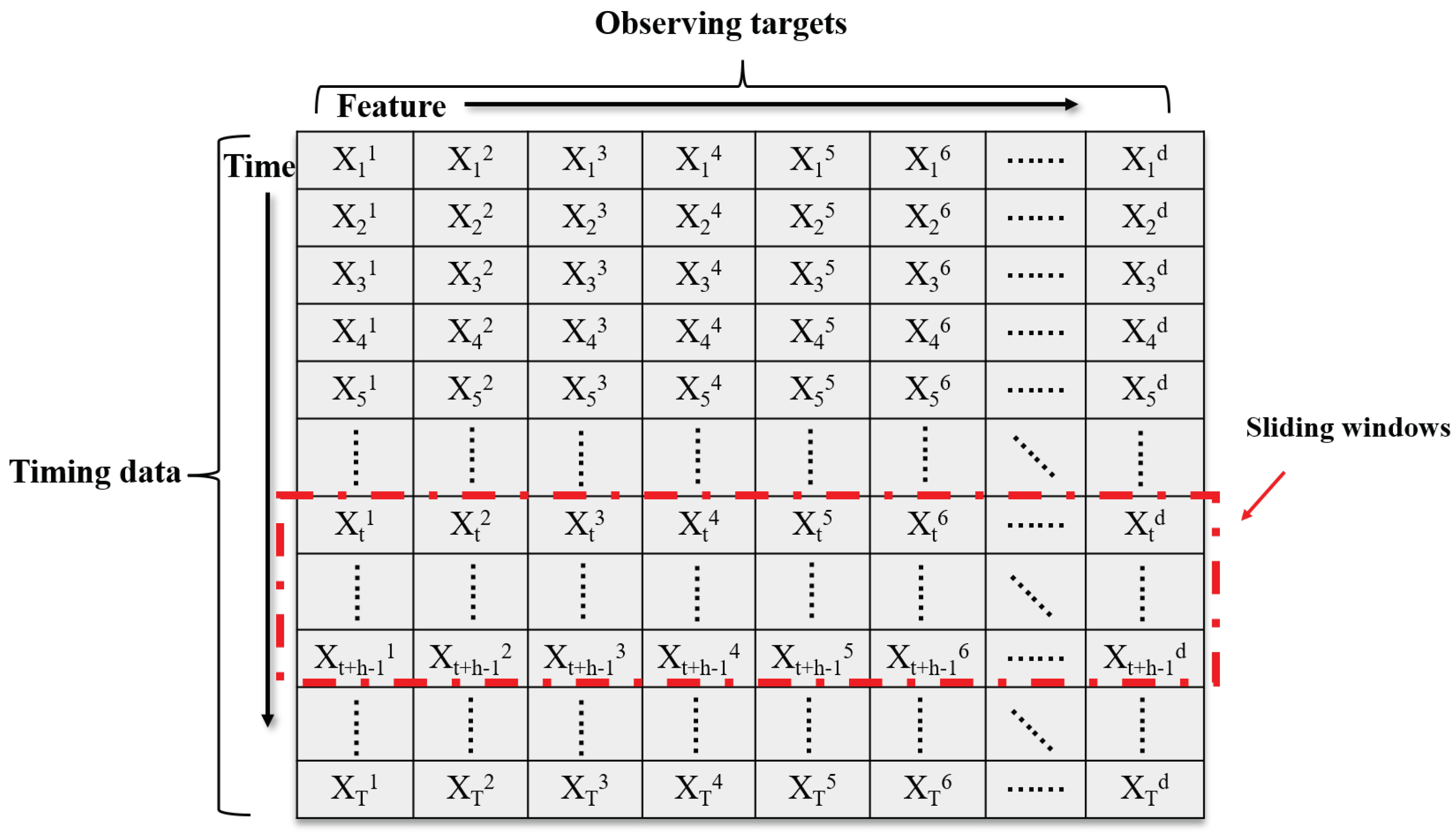
3.1. Problem Statement

A multivariable time series is composed of multiple univariate time series containing dependencies between multiple features. The time series is usually observed under continuous equidistant timestamps, where the input multivariable time series data are $\mathrm{x}\in {\mathbb{R}}^{\mathrm{T}}$, $\mathrm{x}=\left\{{\mathrm{X}}_1,{\mathrm{X}}_2\cdots {\mathrm{X}}_{\mathrm{T}}\right\}$, T is the maximum length of the input timestamp, d is the number of variables for each timestamp, and $\mathrm{x}=\left\{{\mathrm{X}}_{\mathrm{t}}^1,{\mathrm{X}}_{\mathrm{t}}^2,\cdots {\mathrm{X}}_{\mathrm{t}}^{\mathrm{d}}\right\},\mathrm{x}\in {\mathbb{R}}^{\mathrm{T}\times \mathrm{d}}$. See Figure 1.

The tasks of anomaly detection are to obtain the corresponding output vector y by learning the relationship between time series and determine whether the observation value ${\mathrm{y}}_{\mathrm{t}}$ when t is abnormal data through the set threshold, where ${\mathrm{y}}_{\mathrm{t}}\in \{0,1\}$ (1 represents point of abnormal data).

3.2. Data Preprocessing

To avoid the model being affected by extreme values of data, enhance the stability of model training and improve the speed of model learning, we normalize the data in the following ways:

$${\tilde{\mathrm{x}}}_{\mathrm{m},\mathrm{n}}=\frac{{\mathrm{x}}_{\mathrm{m},\mathrm{n}}-min\left({\mathrm{x}}_{\mathrm{n}}\right)}{max\left({\mathrm{x}}_{\mathrm{n}}\right)-min\left({\mathrm{x}}_{\mathrm{n}}\right)+\mathrm{a}}\mathrm{n}\in [1,\mathrm{d}],\mathrm{m}\in [1,\mathrm{T}]$$

(1)

where ${\mathrm{x}}_{\mathrm{m},\mathrm{n}}$ represents the data to be normalized; $min\left({\mathrm{x}}_{\mathrm{n}}\right)$ and $max\left({\mathrm{x}}_{\mathrm{n}}\right)$ are the minimum and maximum values in each column of data, respectively; and then a is the fixed value that prevents the denominator from being 0. All the train and test data are classified into the range of [0, 1], and the processed data are scaled to the specified space, and finally, the data are restored by inverse normalization after the test.

All data are divided into multiple sliding windows as the standard length of data input: ${\omega }_{\mathrm{t}}=\left\{{\mathrm{X}}_{\mathrm{t}},\cdots \cdots ,{\mathrm{X}}_{\mathrm{t}+\mathrm{h}-1}\right\}$. Instead of focusing on the relationship between individual timestamps, the information in the entire sliding window is used to analyze the value of the next timestamp, as shown in Figure 1. Such data input methods can better grasp the time correlation between long time series and avoid the mutation of independent data affecting the detection effect. Anomaly detection results will be obtained from anomaly scores, and the effect of anomaly detection can be evaluated by selecting an appropriate threshold.

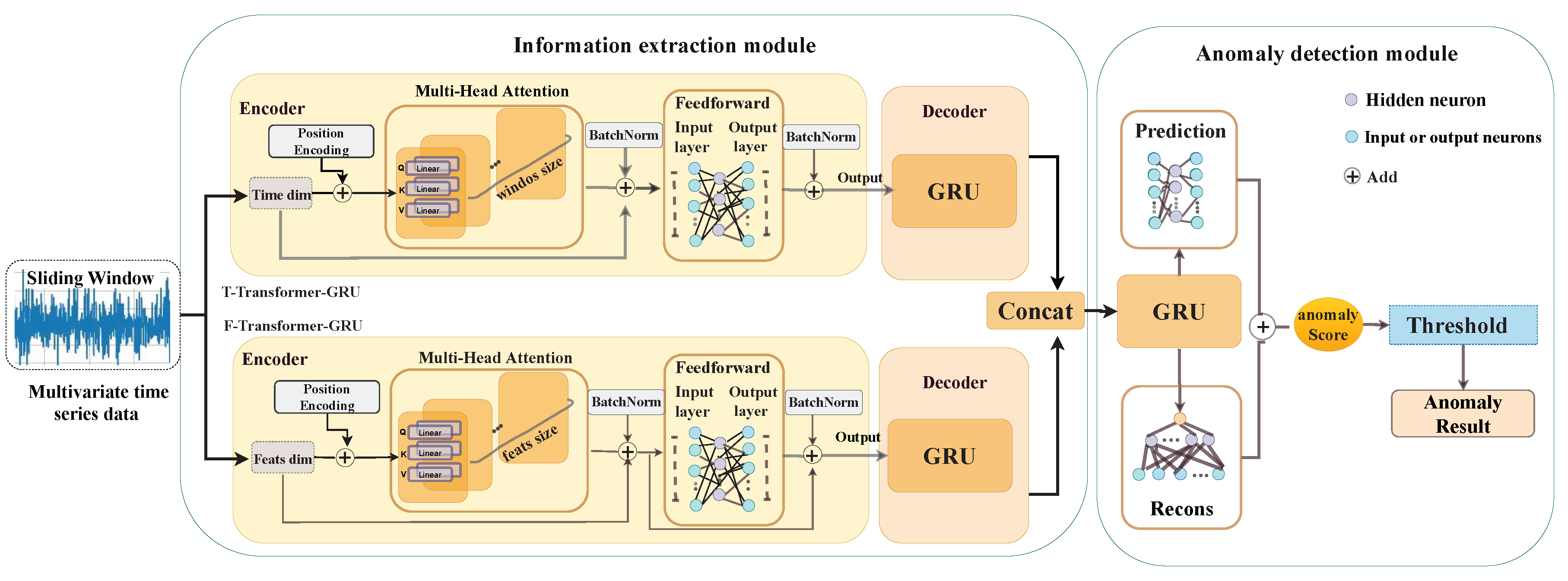
3.3. Anomaly-PTG Network

The Anomaly-PTG model first divides the preprocessed data into multiple data modules in the form of sliding windows and inputs them to the encoding ends of the two transformers. F-transformer GRU utilizes the attention mechanism to conclude the weight of each feature (see Figure 2), extracting the relationship between the current feature and other features.

T-transformer GRU takes each sliding window as an overall input, wields the attention mechanism, and captures the long-distance information dependencies of time series data to conclude information in the time dimension. The GRU, as the decoder of the transformer, is used to update the information and further learn the hidden associations between variables. To aggregate multi-scale information and obtain a better representation of time series, the model concatenates the extracted temporal and feature dimensions to form a new data dimension. The GRU is applied to model the novel time series, and through an autoencoder reduces the dimensions of high-dimensional features and outputs the last hidden layer containing all the previous information. The hidden layer information is passed into the reconstruction and the prediction networks to detect anomalies, respectively; and related detection results are optimized and combined to obtain the total anomaly detection score. Then, through comparison with the threshold, the abnormal detection result is acquired finally.

In addition, because the predicted value is often inaccurate or unpredictable, the reconstruction-based method has a more stable detection effect than the prediction-based method. However, prediction-based methods can also detect anomalies that cannot be captured by reconstruction, so we take the reconstruction method as the main task of our anomaly detection and predict the timestamp anomaly detection of the next stage as a side task. The two steps are performed simultaneously, and the loss function means the weighted sum of the two. The formula of the loss function is as follows:

$${\mathrm{Loss}}_{\mathrm{total}}=\lambda {\mathrm{Loss}}_{\mathrm{recon}}+(1-\lambda ){\mathrm{Loss}}_{\mathrm{pre}}$$

(2)

where ${\mathrm{Loss}}_{\mathrm{total}}$ is the total loss function of the Anomaly-PTG model, ${\mathrm{Loss}}_{\mathrm{recon}}$ is the Loss function based on the reconstruction method, ${\mathrm{Loss}}_{\mathrm{pre}}$ is the loss function based on the prediction method, and $\lambda$ is a pre-set hyperparameter. The final output includes the abnormal scores s$\left\{{\mathrm{S}}_{\mathrm{r}1},{\mathrm{S}}_{\mathrm{r}2}\cdots ,{\mathrm{S}}_{\mathrm{r}\mathrm{T}}\right\}$ obtained from the reconstruction errors, the abnormal scores $\left\{{\mathrm{S}}_{\mathrm{p}1},{\mathrm{S}}_{\mathrm{p}2}\cdots ,{\mathrm{S}}_{\mathrm{p}\mathrm{T}}\right\}$ from the prediction errors, and the total abnormal scores $\left\{{\mathrm{S}}_1,{\mathrm{S}}_2\cdots ,{\mathrm{S}}_{\mathrm{T}}\right\}$.

According to the description of the above model, we give the pseudo-code for training and testing the Anomaly-PTG model in Algorithm 1:

Algorithm 1 Anomaly-PTG model training algorithm:

Input: Train Datasets;

$W=\left\{{\omega }_1\dots \dots ,{\omega }_{\frac{\mathrm{T}}{\mathrm{h}}}\right\}$, parameter $\lambda$ and $\beta$;

Output: Trained Anomaly-PTG model;

EPOCH ← 1; Labels y = {y1, y2 … yt … yt+k};

for t in range (t + k) do:

$\mathrm{prediction}{\widehat{\mathbf{y}}}_{\mathrm{t}+1,\mathrm{i}}\leftarrow \mathbf{Anomaly}\mathbf{‒}\mathbf{PTG}\left({\widehat{\mathbf{y}}}_{\mathrm{ti}}\right);$

$\mathrm{recons}{\widehat{\mathrm{x}}}_{\mathrm{t}+\mathrm{L},\mathrm{i}}\leftarrow \mathbf{Anomaly}\mathbf{‒}\mathbf{PTG}\left({\mathrm{x}}_{\mathrm{t},\mathrm{i}}\right);$

${\mathrm{loss}}_{\mathrm{total}}=\lambda {loss}_{\mathrm{recon}}+(1-\lambda ){loss}_{\mathrm{pre}}$;

$\mathbf{Anomaly}\mathbf{-}\mathbf{PTG}\leftarrow \mathrm{update}\mathrm{weight}\mathrm{using}\mathrm{loss};$

end for

epoch ← epoch + 1

UNTIL epoch = end;

Test Anomaly-PTG model;

Threshold bf = Brute-force Algorithm;

for j = (t + k + 1) in range T

${\mathrm{S}}_{\mathrm{j}}={\sum }_{\mathrm{i}}^{\mathrm{feats}}\left(\sqrt{{\left({\widehat{\mathrm{y}}}_{\mathrm{t},\mathrm{i}}-{\mathrm{x}}_{\mathrm{t},\mathrm{i}}\right)}^2}+\beta \sqrt{\left.{\left({\widehat{\mathrm{x}}}_{\mathrm{t},\mathrm{i}}-{\mathrm{x}}_{\mathrm{t},\mathrm{i}}\right)}^2\right)}\right.;$

$\mathrm{If}{\mathrm{S}}_{\mathrm{j}}>\mathrm{bf}\mathbf{then}$

${\mathrm{y}}_{\mathrm{j}}=1;$

$\mathbf{else}$

${\mathrm{y}}_{\mathrm{j}}=0;$

$\mathbf{end}\mathbf{if}$

$\mathbf{end}\mathbf{for}$

3.4. Information Extraction Module

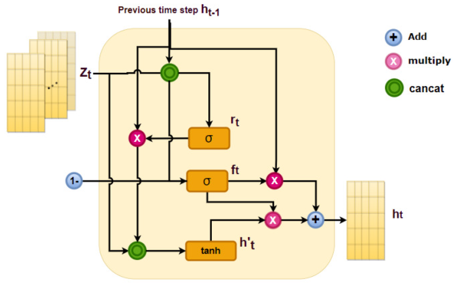
Transformer-GRU

Encoder: The transformer relies on the attention mechanism to catch the relationship between contexts well and can preferably model sequence data. The training speed of the model is improved by this method. In this part, the structure of the transformer is enhanced and applied to anomaly detection tasks on multivariable time series. As shown in Figure 3, the T-transformer GRU and F-transformer GRU capture the time correlation and feature correlation of multivariate time series data, respectively. Through the multi-head attention mechanism, it obtains the relationship between each feature and the long-distance time hiding information between time series data. Next is the formula explanation of this part. Firstly, the established three matrices, ${\mathrm{M}}_{\mathrm{Q}}$, ${\mathrm{M}}_{\mathrm{K}}$, and ${\mathrm{M}}_{\mathrm{V}}$, are denoted as query matrix Q, key matrix K, and value matrix V, respectively. The calculation formula for self-attention is

$$\mathrm{A}\mathrm{t}\left({\mathrm{M}}_{\mathrm{Q}},{\mathrm{M}}_{\mathrm{K}},{\mathrm{M}}_{\mathrm{V}}\right)=\sigma \left(\frac{{\mathrm{M}}_{\mathrm{Q}}{\mathrm{M}}_{\mathrm{K}}{}^{\mathrm{T}}}{\sqrt{\mathrm{a}}}\right){\mathrm{M}}_{\mathrm{V}}$$

(3)

where $\sigma$ denotes the softmax activation function, which maps the weights we obtain into [0, 1], and $\sqrt{\mathrm{a}}$ is used to scale the weights to enhance the stability of training.

In the F-transformer GRU, we regard the features of each timestamp as our word vector and calculate the weight between the various features in the input ${\mathrm{x}}_{\mathrm{i}}$ ($\mathrm{i}\in \mathrm{f}\mathrm{e}\mathrm{a}\mathrm{t}\mathrm{s}$, the input has been added to the position encoding), and the calculation formula is

$$\begin{array}{c}\mathrm{K}={\displaystyle \sum _{\mathrm{i}=1}^{\mathrm{feats}}}{\mathrm{k}}_{\mathrm{i}}={\displaystyle \sum _{\mathrm{i}=1}^{\mathrm{feats}}}{\mathrm{x}}_{\mathrm{i}}\ast {\mathrm{M}}_{\mathrm{K}}\\ {\mathrm{a}}_{\mathrm{i}}=\sigma \left({\mathrm{K}}^{\mathrm{T}}{\mathrm{q}}_{\mathrm{i}}\right)\end{array}$$

(4)

where ${\mathrm{a}}_{\mathrm{i}}$ is the weight between the current feature and other features. We obtain the relationship between each feature in each input timestamp. $\sigma$ denotes the softmax activation function; ${\mathrm{k}}_{\mathrm{i}}$ and ${\mathrm{q}}_{\mathrm{i}}$, respectively, represent the key vector and query vector representation obtained after the current feature is multiplied by its key matrix ${\mathrm{M}}_{\mathrm{K}}$ and query matrix ${\mathrm{M}}_{\mathrm{Q}}$.

$$\sum _{\mathrm{i}=1}^{\mathrm{feats}}{\mathrm{Z}}_{\mathrm{i}}={\mathbf{a}}_{\mathbf{i}}\ast {\mathrm{v}}_1+{\mathbf{a}}_{\mathbf{i}}\ast {\mathrm{v}}_2+\cdots +{\mathbf{a}}_{\mathbf{i}}\ast {\mathrm{v}}_{\mathrm{feats}}$$

(5)

where ${\mathrm{v}}_{\mathrm{i}}$ represents the value vector representation obtained by multiplying the current characteristic by its value matrix ${\mathrm{M}}_{\mathrm{V}}$, and ${\mathrm{Z}}_{\mathrm{i}}$ is the final output of the current feature calculated by the self-attention mechanism.

As for this model, we utilize the multi-head attention mechanism:

$$\mathrm{MultiAt}(\mathrm{Q},\mathrm{K},\mathrm{V})=Concat\left(\mathrm{A}{\mathrm{t}}_1,\mathrm{A}{\mathrm{t}}_2,\dots ,\mathrm{A}{\mathrm{t}}_{\mathrm{feats}}\right)$$

(6)

Turning a set of original ${\mathrm{M}}_{\mathrm{Q}}$, ${\mathrm{M}}_{\mathrm{K}}$, and ${\mathrm{M}}_{\mathrm{V}}$ into multiple sets of such matrices means that we can focus on the information of the input matrix from multiple spaces, and graph the feature relationship of the data from multiple perspectives. The obtained ${\mathrm{Z}}_{\mathrm{i}}$ and ${\mathrm{X}}_{\mathrm{i}}$ are residually connected into a variable ${\mathrm{X}}_{\mathrm{attention}}$ with attention and are normalized. We use batch normalization ${\widehat{\mathrm{x}}}_{\mathrm{attention}}=\mathrm{BatchNorm}\left({\mathrm{X}}_{\mathrm{attention}}\right)$, which can reduce the interference of outliers and become more suitable for time-series-anomaly detection tasks [38]. Pass the normalized data through a feedforward neural network for linear activation.

$$\begin{array}{ll}\hfill & {\widehat{\mathrm{x}}}_{\mathrm{attention}}^{\prime }=ReLU(Linear\left({\widehat{\mathrm{x}}}_{\mathrm{attention}}\right)),ReLU=max(0,\mathrm{x})\hfill \\ \hfill & {\mathrm{X}}_{\mathrm{FeedForward}}=Linear\left({\widehat{\mathrm{x}}}_{\mathrm{attention}}^{\prime }\right)\hfill \\ \hfill & \mathrm{Z}=\mathrm{BatchNorm}\left({\widehat{\mathrm{x}}}_{\mathrm{attention}}+{\mathrm{X}}_{\mathrm{FeedForward}}\right)\hfill \end{array}$$

(7)

We combine the full connection layer and the relu activation function in the feedforward network. RelU activation function is a nonlinear function, which can learn complex relationships in data, so it can better map the nonlinear layer. The idea is that if the input is greater than zero, it is directly the return value. If the input is 0 or less, the return value is 0. The advantage of this is that the network training can be faster and effectively prevent the gradient’s disappearance. In this network, two linear layers are used. The function of these two linear layers is a process of first mapping data to a higher dimensional space and then to a lower dimensional space so that more abstract features can be learned.

Finally, the output of the feedforward neural network is connected with ${\widehat{\mathrm{x}}}_{\mathrm{attention}}$ and batch normalized again as the final output result Z. BatchNorm is a data-normalization method that can standardize the input and hidden layer data to reduce the differences between samples. He normalized the data by first asking for the mean and variance of each batch of data, and then subtracting the mean from the data and dividing it by the variance. In the past, the transformer LayerNorm was used, which is generally suitable for NLP tasks. After applying a transformer to time-series anomaly detection, we found that BatchNorm has a better effect than LayerNorm because it can effectively avoid the influence of outliers in time series data, which is different from that used in NLP tasks to deal with the relationship between sentences. Therefore, BatchNorm is a more suitable normalization processing method for time series data.

We catch the potential correlation of features in the multivariable time series through the encoder end of the F-transformer GRU. Similarly, in T-transformer GRU, referring to time series data, we take the time dimension of the sliding window as input to capture long-range temporal dependencies.

Decoder: Anomaly-PTG decodes the correlation information extracted by the encoder side through the GRU to conclude a better time series representation, which is a more suitable structure for exception detection tasks.

RNN is a common method in time-series anomaly detection. However, its disadvantage is that it cannot capture the long-distance sequence information and is prone to gradient disappearance and gradient explosion. Therefore, LSTM and GRU models are proposed based on RNN. By using the gating mechanism, the defects of RNN are well solved. Since GRU reduces the number of parameters by 1/4 compared with LSTM, it is more efficient and more straightforward in light of structure than LSTM in the model training process. Thus, instead of LSTM, GRU is applied in our model to obtain the information in the input data and the sequential representation (see Figure 4).

GRU comprises two parts: the reset gate ${\mathrm{r}}_{\mathrm{t}}$ and update gate ${\mathrm{f}}_{\mathrm{t}}$. As Figure 4 shows, we take the output ${\mathrm{Z}}_{\mathrm{t}}$ of the encoder as the input of GRU at the current moment. By using the update gate, the irrelevant features at the previous time are ignored while important features are retained, and the formula is as follows:

$$\begin{array}{c}{\mathrm{f}}_{\mathrm{t}}=\sigma \left({\mathrm{W}}_{\mathrm{f}}·\left[{\mathrm{h}}_{\mathrm{t}-1,\mathrm{Zt}}\right]\right),\\ {\mathrm{r}}_{\mathrm{t}}=\sigma \left({\mathrm{W}}_{\mathrm{r}}·\left[{\mathrm{h}}_{\mathrm{t}-1,\mathrm{Zt}]}\right),\right.\\ {\mathrm{h}}_{\mathrm{t}}^{\prime }=tanh\left(\mathrm{W}·\left[{\mathrm{r}}_{\mathrm{t}}\ast {\mathrm{h}}_{\mathrm{t}-1},{\mathrm{zt}}_{\mathrm{t}}\right]\right),\\ {\mathrm{h}}_{\mathrm{t}}={\left(1-{\mathrm{f}}_{\mathrm{t}}\right)}^{\ast }{\mathrm{h}}_{\mathrm{t}-1}+{\mathrm{f}}_{\mathrm{t}}\ast {\mathrm{h}}_{\mathrm{t}}^{\prime }\end{array}$$

(8)

where [ ] denotes cancat, · denotes matrix multiplication, and $\sigma$ denotes the sigmoid activation function. The update gate ${\mathrm{f}}_{\mathrm{t}}$ is used to control the influence of the hidden layer information ${\mathrm{h}}_{\mathrm{t}-1}$ retained at the previous moment on the input ${\mathrm{Z}}_{\mathrm{t}}$ at the current moment, and the reset gate ${\mathrm{r}}_{\mathrm{t}}$ is used to forget the irrelevant information of the previous moment and the current moment according to the current input; ${\mathrm{h}}_{\mathrm{t}}^{\prime }$ records the state learned at the current moment, and finally the hidden layer state h at the current moment.

3.5. Anomaly Detection Module

3.5.1. Reconstruction Network

We concatenate the output of the parallel transformer GRU, then input it into a GRU. An autoencoder network based on GRU is built for reconstruction. In this part, we first re-encode its hidden layer ht into the same shape as the original data and then input it into the GRU model. The GRU learns the information representation of the hidden vector at the encoding end and then decodes it. The decoded latent vector ${\mathrm{h}}_1\cdots {\mathrm{h}}_{\mathrm{windos}\mathrm{size}}$ is used as the output x of the GRU, and finally, the output is passed to the fully connected layer as the output $\widehat{\mathrm{x}}$ of the reconstructed model. The loss function of reconstruction is the root mean square error (RMSE), i.e.,

$${loss}_{\mathrm{recon}}=\sqrt{\sum _{\mathrm{i}=1}^{\mathrm{feats}}{\left({\widehat{\mathrm{x}}}_{\mathrm{t},\mathrm{i}}-{\mathrm{x}}_{\mathrm{t},\mathrm{i}}\right)}^2}$$

(9)

where ${\widehat{\mathrm{x}}}_{\mathrm{t},\mathrm{i}}$ denotes the reconstructed value of the feature of i for the current timestamp t, and ${\mathrm{x}}_{\mathrm{t},\mathrm{i}}$ denotes the real value corresponding to the current timestamp t.

3.5.2. Threshold Selection

To testify the best anomaly detection effect of the Anomaly-PTG model, we use brute-force, which is a threshold selection method mentioned in the OmniAnomaly model, to find the best F1 value of the model and return the most appropriate threshold.

The specific steps are as follows. We start by setting a threshold range; the threshold is updated through iteration to calculate the F1 values in light of different thresholds, find the best F1 value, and return to get the threshold of this result. The pseudocode is shown in Algorithm 2:

Algorithm 2 Brute-force Algorithm:

Input:

anomaly_scores, true_anomalies, start = 0.01, end = 2, step_num = 100;

Output:

Finding best f1 = bf;

search_step, search_range, search_lower_bound = step_num, end-start, start;

threshold = search_lower_bound;

m = (0.0, 0.0), m_t = 0.0;

for i in range (search_step):

threshold += search_range / float(search_step);

target←Calculate the F1 of the current threshold;

if target[0] > m[0]: ← Compares whether the current F1 is the highest;

m_t = threshold;

m = target;

end for

gain threshold = bf;

3.5.3. Prediction Network

The loss function used by our prediction network is the root-mean square error (RMSE), and its formula is listed as follows:

$${\mathrm{loss}}_{\mathrm{pre}}=\sqrt{\sum _{\mathrm{i}=1}^{\mathrm{feats}}{\left({\widehat{\mathrm{y}}}_{\mathrm{t},\mathrm{i}}-{\mathrm{x}}_{\mathrm{t},\mathrm{i}}\right)}^2}$$

(10)

where feats is the number of features in the dataset, ${\widehat{\mathrm{y}}}_{\mathrm{t},\mathrm{i}}$ represents the predicted value of the i-th feature at the current timestamp t, and ${\mathrm{x}}_{\mathrm{t},\mathrm{i}}$ represents the actual value corresponding to the expected value. We pass the output of the GRU into a fully connected layer as a prediction network to predict the value for the next timestamp.

3.5.4. Anomaly Scores

Finally, we combine the above reconstruction error with the prediction error to get the final anomaly scores for the current timestamp t, whose formula is as follows:

$$\mathrm{anomaly}\mathrm{scores}=\frac{{\sum }_{\mathrm{i}}^{\mathrm{feats}}{\mathrm{s}}_{\mathrm{i}}}{\mathrm{feats}}=\frac{{\sum }_{\mathrm{i}}^{\mathrm{feats}}\left(\sqrt{{\left({\widehat{\mathrm{y}}}_{\mathrm{t},\mathrm{i}}-{\mathrm{x}}_{\mathrm{t},\mathrm{i}}\right)}^2}+\beta \sqrt{\left.{\left({\widehat{\mathrm{x}}}_{\mathrm{t},\mathrm{i}}-{\mathrm{x}}_{\mathrm{t},\mathrm{i}}\right)}^2\right)}\right.}{\mathrm{feats}}$$

(11)

Among them, we set $\beta$ as a hyperparameter to optimize the combined effect of the prediction task and the reconstruction task, and the optimal combination ratio will be obtained through experiments. In Section 4.7, we present the analysis results of the effect of different $\beta$ values on the model.

4. Experiment and Analysis

4.1. Datasets

Four public datasets were employed in our experiments. We describe the dataset information in detail in

Table 1. Summary of dataset information.

Attributes	SMAP	MSL	SMD	KDDCUP99
Entity	55	27	28	-
Dimension	25	55	38	41
Train data	135,183	58,317	708,405	311,028
Test data	427,617	73,729	708,420	494,020
Abnormal rate	13.13%	10.72%	4.16%	19.69%

, where the first column represents the attributes for each dataset. Entity represents the number of entities observed in the dataset, and Dimension is the number of dimensions contained in each entity. The remainder includes the training and test data and the proportion of abnormal data in the test dataset.

We included SMAP (Soil Moisture Active Passive) [7], MSL (Mars Science Laboratory) [7], and SMD (Server Machine Dataset) [18] for comparative experiments. Our model was used for the KDDCUP99 [39], a network intrusion detection dataset, to prove the generalization ability.

(1) SMAP and MSL

These two datasets are from observation satellite data collected by NASA, and SMAP transmits observation data through active and passive sensors. MSL contains the data sent back by the Mars probe, similar to SMAP data. Their data are divided into training set and test sets, in which the abnormality of the test set has been marked.

(2) SMD

SMD contains the server data provided by a large Internet company for five weeks. The main observation is the resource utilization of each machine in the computer cluster. At present, the dataset has been released on GitHub.

(3) KDDCUP99

The KDDCUP99 dataset is a network intrusion detection dataset captured by the DARPA ’98 IDS evaluation program, which is classified as normal data or attacks. The test dataset consists of 24 training attack types and 14 attack types, and the abnormal data are labeled.

4.2. Evaluation Metrics

This section introduces the evaluation index of the model and regards the F1 and area under the ROC curve (AUC) as the standards for anomaly detection performance. Precision (P), recall (R), F1-score (F1), AUC, and recall at 90% precision(R*) are used for reporting in the evaluation of this work, and the calculation formula is as follows:

$$\begin{array}{cc}\hfill & \mathrm{Precision}=\frac{\mathrm{TP}}{\mathrm{TP}+\mathrm{FP}}\hfill \\ \hfill & \mathrm{Recall}=\frac{\mathrm{TP}}{\mathrm{TP}+\mathrm{FN}}\hfill \\ \hfill & \mathrm{F}1-\mathrm{score}=\frac{2\times \mathrm{Precision}\times \mathrm{Recall}}{\mathrm{Precision}+\mathrm{Recall}}\hfill \\ \hfill & \mathrm{AUC}=\frac{1}{2}\sum _{\mathrm{i}=1}^{\mathrm{m}-1}\left({\mathrm{x}}_{\mathrm{i}+1}-{\mathrm{x}}_{\mathrm{i}}\right)\left({\mathrm{y}}_{\mathrm{i}}+{\mathrm{y}}_{\mathrm{i}+1}\right)\hfill \end{array}$$

(12)

TP means true positives, that is, normal data in the data are judged as normal; FP is false positives, that is, abnormal data in the data are judged as normal; FN is false negatives, which means normal data in the data are judged as abnormal; TN is true negatives. Note that y is the true positive rate ($\mathrm{TPR}=\frac{\mathrm{TP}}{\mathrm{TP}+\mathrm{FN}}$) and x is the false positive rate ($\mathrm{FPR}=\frac{\mathrm{FP}}{\mathrm{FP}+\mathrm{TN}}$).

In some factual situations, anomaly omissions may lead to irreparable losses. Therefore, in the design of some anomaly detection models, it is allowed to sacrifice some precision to improve the recall rate to meet the requirement of not letting go of any anomaly. Given this actual demand, we adjusted the threshold to make the precision of all baseline methods consistent. Verify the model’s recall rate under the condition of meeting the high precision required by anomaly detection. We must ensure the model’s precision to avoid interference with normal data. In our study, a precision of over 90% was necessary to deploy the model. Therefore, we fixed the precision at 90% and verified the recall rate (R*) of all models on this basis to prove the practical value of the models.

4.3. Experimental Parameters and Baseline Methods

Our proposal is compared with some advanced methods, including DAGMM [14], USAD [25], OmniAnomaly [18], MAD-GAN [24], GDN [21], TranAD [35], and MTAD-GAT [11]. The implementation environment was Pytorch version 1.10.2, CUDA 11.4, NVIDIA Tesla A100 GPUs×1, and Xeon 2.59 GHz CPU × 1. Each dataset was trained for 100 epochs. The specific parameters are shown in

Table 2. Parameter configuration.

Parameters	Value
window size	100
batch_size	128
Number of layers in GRU	1
Number of layers in Recon network	1
Fully-connected layers	4
Number of layers in transformer GRU	1
GRU hidden dimension	300
Forecast hidden dimension	300
Recon network hidden dimension	300
$\beta$	1.2
$\lambda$	0.7
epochs	100

. The optimal values of hyperparameters $\beta$ and $\lambda$ were 1.2 and 0.7, respectively. The learning rates of the SMAP and MSL were 1 × 10${}^{-4}$; SMD was 1 × 10${}^{-3}$; KDDCUP99 was 1 × ${10}^{-5}$.

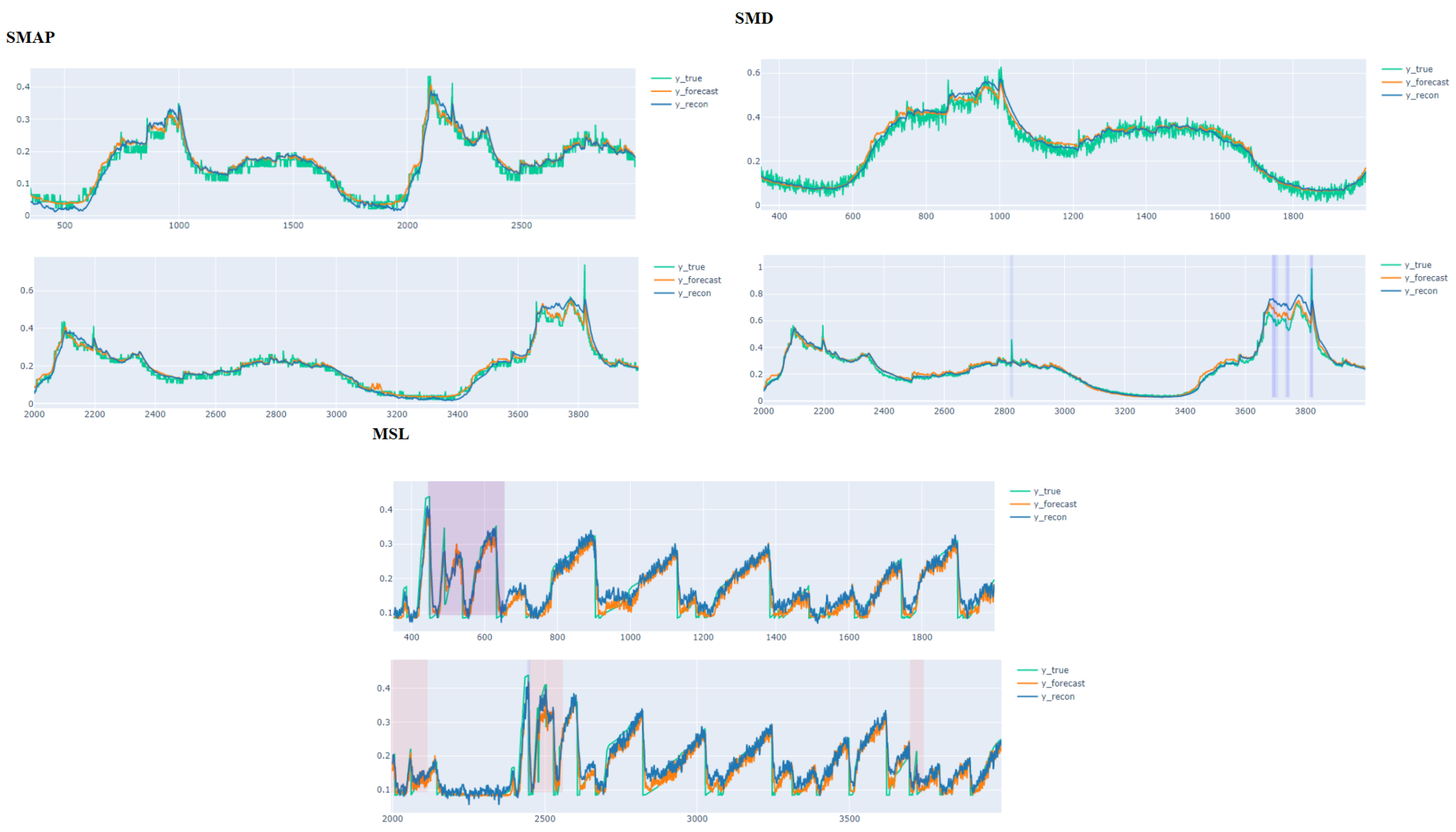
4.4. Results and Analysis

The comparison results between Anomaly-PTG and the baseline model are shown in

Table 3. Anomaly-PTG comparison with baseline method.

Datasets	Methods	P	R	F1	AUC	R*
SMD	DAGAMM	0.8872	0.9752	0.9291	0.9838	0.9602
	USAD	0.9059	0.9814	0.9421	0.9857	0.9842
	OmniAnomaly	0.8784	0.9485	0.9120	0.9780	0.9138
	MAD−GAN	0.9994	0.7270	0.8417	0.9843	0.8279
	GDN	0.7469	0.9618	0.8408	0.9799	0.9063
	TranAD	0.9072	0.9973	0.9501	0.9862	0.9978
	MTAD−GAT	0.8412	0.9417	0.8886	0.9831	0.8947
	Anomaly−PTG	0.9692	0.9873	0.9781	0.9907	0.9988
MSL	DAGAMM	0.7363	0.9648	0.8352	0.9618	0.7883
	USAD	0.8048	0.9810	0.8842	0.9736	0.8965
	OmniAnomaly	0.7942	0.9897	0.8825	0.9697	0.9076
	MAD−GAN	0.8516	0.9921	0.9164	0.9733	0.9412
	GDN	0.8908	0.9917	0.9385	0.9789	0.9846
	TranAD	0.9037	0.9999	0.9494	0.9807	0.9995
	MTAD−GAT	0.8189	0.9888	0.8958	0.9874	0.9243
	Anomaly−PTG	0.9599	0.9412	0.9505	0.9846	0.9909
SMAP	DAGAMM	0.8069	0.9912	0.8896	0.9722	0.9172
	USAD	0.7998	0.9627	0.8737	0.9796	0.8779
	OmniAnomaly	0.8008	0.9638	0.8747	0.9748	0.8934
	MAD−GAN	0.8257	0.9579	0.8869	0.9807	0.8846
	GDN	0.8192	0.9452	0.8777	0.9812	0.8667
	TranAD	0.8043	0.9999	0.8915	0.9842	0.9265
	MTAD−GAT	0.8666	0.9406	0.9021	0.9776	0.9138
	Anomaly−PTG	0.9210	0.9690	0.9443	0.9894	0.9743

. The highest score is shown in bold. We regard the F1 value and AUC as the criterion for judging the model’s performance. According to the table, our model obtains excellent results on all three datasets. Anomaly-PTG is better than the baseline methods of all datasets except MSL (in terms of F1 scores and AUC). As the time series data in MSL dataset contain more features, the recognition ability of each method is very different. For this dataset, Anomaly-PTG’s F1 score was 0.11% higher than that of the next best baseline method, and the AUC value (0.9846) was only 0.28% lower than that of the best MTAD-GAT model. The other five indicators reached more than 90%. It can be seen that DAGMM only pays attention to the relationship with each variable, but does not consider the relationship in the time dimension, because it adopts the method of inputting single data item by item. Hence, it has a poor performance in identifying anomalies. It can be seen that the effect of capturing remote time dependency by T-transformer GRU can be well reflected in the data.

The limitation of OmniAnomaly is that it does not capture the relationships between variables. In the multivariate-time-series anomaly detection task, the potential influence between variables is the key to anomaly detection. Two methods based on the graph structure, GDN and mad-gat, showed good results in various tasks. It can be seen that the graph structure can effectively extract the relationship between features in time series data. However, because GDN is sensitive to the model’s data and is limited by the sliding window, it cannot get the information of the remote timestamp, which leads to the poor performance of GDN on SMD and SMAP datasets. For the SMAP dataset, Anomaly-PTG, except for the recall indicator, achieved the best results of all baseline methods. From the AUC (0.9894) and F1 (0.9443) values, it can be seen that Anomaly-PTG has shown strong performance for this huge unbalanced dataset of positive and negative samples, increasing the AUC by 0.52% and F1 by 4.22% compared with the best baseline model. For the SMD dataset, MAD-GAN has the best P value (0.9994), and Anomaly-PTG is slightly behind this method. However, for its AUC (0.9907) and F1 value (0.9781), we can see that it still showed the best detection performance of all methods. This is because Anomaly-PTG can simultaneously consider the correlation between features and the remote time dependence of time series data.

Our model captures the correlation between features through an F-transformer GRU and uses the T-transformer GRU that captures long-range temporal dependencies to achieve the most comprehensive information extraction. The results of TranAD and Anomaly-PTG show that the improved transformer’s feature extraction ability is helpful in time-series anomaly detection. Anomaly-PTG combines the associations and long-range temporal dependencies between the extracted features, inputs them into GRU to learn the sequential representation of time series data, and then comprehensively detects anomalies by combining reconstruction and prediction. The result is more stable than TranAD because it is easy to ignore an anomaly with minimal reconstruction error only by the reconstruction method, and the combination of the prediction method will make up for this defect and improve the detection accuracy. As shown in Figure 5, three dataset detection effects of the Anomaly-PTG model is listed. Green represents the actual data; yellow and blue represent the predicted data, and the reconstructed information, respectively. It can be seen that both prediction and reconstruction simulate the data distribution well and complement each other to a certain extent. By optimizing the combination of the two, anomalies can be better detected.

In this experiment, we also considered the problems with applying the model to real scenes. From the experimental results, we can see that the F1-scores of some models perform are good, but the recall rate is poor. For example, see the results of MAD-GAN and GDN. This is because these models focus more on accuracy but are less effective at catching exceptions. Many outliers are mistaken for normal values, leading to abnormal omissions. In some practical application scenarios, the failure to detect exceptions will lead to significant losses. Therefore, many models focus more on improving the recall rate during design. In this regard, we fixed all baseline methods to the same accuracy (90% accuracy) and evaluated each model’s ability to identify anomalies through the recall rate (R*). This is a metric that assesses the utility performance of the model. It can be seen from Table 3 and

Table 4. The anomaly-PTG model was compared with baseline method on the KDDCUP99 dataset.

Datasets	Methods	P	R	F1	AUC	R*
KDDCUP99	DAGAMM	0.8872	0.9973	0.9390	0.8790	0.9780
	USAD	0.9845	0.9465	0.9651	0.8846	0.9927
	OmniAnomaly	0.9015	0.8329	0.8658	0.8613	0.8554
	MAD−GAN	0.8963	0.7465	0.8145	0.8778	0.7368
	GDN	0.9124	0.9673	0.9345	0.8565	0.9781
	TranAD	0.9518	0.9814	0.9664	0.9068	0.9999
	MTAD−GAT	0.9109	0.9862	0.9471	0.8779	0.9974
	Anomaly−PTG	0.9869	0.9590	0.9727	0.9112	0.9999

that the R* of Anomaly-PTG was the highest for all three datasets except the MSL dataset. TranAD performed best on the MSL dataset, and Anomaly-PTG slightly lagged behind with this indicator. The R* of Anomaly-PTG proposed in this paper can reach more than 95% on four datasets, which meets the requirement for exception capturing in practical application scenarios and proves that the model has good practicability.

4.5. Generalization Ability Test

We also used the model for the KDDCUP99 dataset and tested the above baseline methods on this dataset. Referring to Table 4, the F1 value (0.9727) and AUC (0.9112) of the Anomaly-PTG are the highest among all baseline models. The characteristics of KDDCUP99 include the port number, the number of visits, the login information, connection time, and so on, which are more closely correlated. Anomaly-PTG also performed very well on KDDCUP99, demonstrating that the model can detect time-series anomalies in different scenes with more extraordinary generalization ability.

4.6. Ablation Study

This paper considers the correlation between variables in time series data and the relationship between long-distance time information and improves the transformer’s structure to enhance the information extraction ability and make it more suitable for the time-series anomaly detection task. We verify the validity of each part of the Anomaly-PTG model. Ablation results on different datasets were obtained (

Table 5. The ablation results (F1) of each part of the model on different datasets.

Technology	Time	Feats	SMD	MSL	SMAP	KDDCUP99	AVGF1
Transformer	—	w/o	0.9189	0.8742	0.8727	0.8923	0.8895
	w/o	—	0.8812	0.9031	0.8881	0.9299	0.9005
	—	—	0.9578	0.9253	0.9163	0.9518	0.9378
Parallel Transformer-GRU	—	—	0.9781	0.9505	0.9443	0.9727	0.9614

The values in the table represent F1 values. “—” represents the use of this structure. “w/o” represents the not use of this structure.

), where “—” and “w/o” indicate using or not using the technique. Time and feats denote structures for extracting time information and feature relationships. Technology means the technology we used in this study. That is to say, parallel transformer GRU is our improved structure for the transformer.

We replace the structure of extracting global information of the Anomaly-PTG model with the transformer as the model’s basic structure. It can be concluded from the table that extracting only temporal information or extracting only relations between features has a different performance on the dataset. For example, each feature contains a large amount of continuous time series data in the SMD dataset. In anomaly detection, it is essential to extract long-distance time information. Therefore, as can be seen in the second row of the table, the F1 value of the model is reduced by 7.6% in the SMD dataset without considering the time information.

MSL dataset has the most features, so it is necessary to extract the potential correlations between the features of this dataset for anomaly detection. In the first row of the table, we can see that the F1 value of the model on the MSL dataset decreases by 3.9% due to not using the structure that captures the feature relationship. For the third row, we extract temporal information and feature relationships to improve the stability and accuracy of the model in different scenarios, and the average F1 value on the three datasets was improved by 3.7% and 4.8%, respectively. It had good performance on each dataset, proving the two-part connection’s effectiveness. Subsequently, we replaced the transformer’s structure with a parallel transformer GRU structure. It can be seen that the improved transformer is more suitable for extracting information from time series data and achieves the best results, including an average F1 improvement of 2.3% over the previous transformer. The validity of this method is further proved.

In

Table 6. Ablation results (F1) on different datasets based on reconstruction and prediction methods.

Technology	Recon	Predicet	SMD	MSL	SMAP	KDDCUP99	AVGF1
	—	w/o	0.9553 t	0.8961	0.9284	0.9583	0.9345
Parallel Transformer-GRU	w/o	—	0.9665	0.8366	0.8657	0.9023	0.8927
	—	—	0.9781	0.9505	0.9443	0.9727	0.9614

, Recon and Predict represent reconstruction and prediction networks in the model, respectively. We prove the effectiveness of combining prediction and reconstruction by controlling variables. In light of the ablation results, we know that both the prediction-based anomaly detection and the reconstruction-based anomaly detection alone are not as good as the combined detection methods, and the F1 score decreased by 6.8% and 2.69% on average, respectively. This is because prediction-based anomaly detection becomes more sensitive to the detection data, and the performance of predicting anomalies in different scenarios varied greatly, resulting in unstable detection performance of the model. The method based on reconstruction is to study the probability distribution of the data, which has lower requirements on the data type. Therefore, the way based on reconstruction is often more stable than the method based on prediction. Still, the technique based on reconstruction easily ignores abnormal data of minor reconstruction errors. Therefore, according to the importance of the task, the reconstruction is used as the main task of the model to detect abnormal data, and the prediction-based method is applied to assist the reconstruction of the anomalies that cannot be captured. The specific analysis is shown in Figure 6.

The figure shows data fluctuations between different features in the test set. The three lines are the predicted value, the reconstructed value, and the actual value, respectively. The prediction-based model can directly indicate the data of the following timestamp by using the time series data’s time dependence. The reconstruction-based model helps capture the global data distribution and can more accurately judge the abnormality according to the normal distribution of the data. Still, it is not easy to identify sudden data fluctuations because these fluctuant data may also conform to the normal data distribution, leading to missed abnormal detection. As marked by the red box in Figure 6, the prediction model can capture this mutation data, and the reconstruction-based approach does not capture this anomaly.

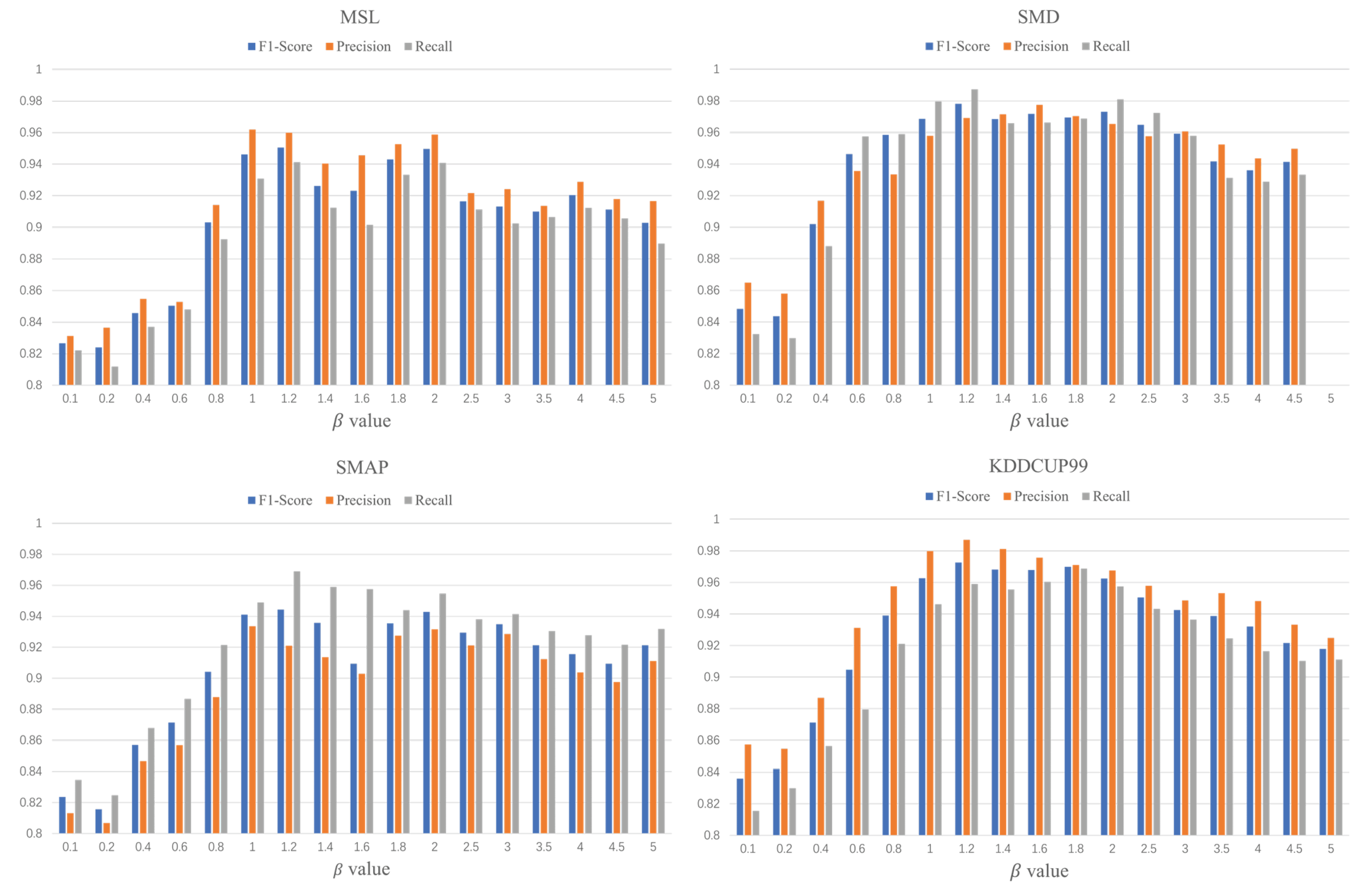
4.7. Parametric Analysis

$\beta$ analysis:$\beta$ is the parameter that regulates the optimal combination of prediction and reconstruction methods. We combined the two methods to assign weights based on the sensitivity of abnormal data and found that different values will have a particular impact on the detection effect. Therefore, we conducted extensive experiments to evaluate the F1 value, recall, and precision of other $\beta$ on four datasets. The results are shown in Figure 7. When the $\beta$ value is 1.2, the F1 value shows the best results on the four datasets. When the $\beta$ value is less than 1, the detection accuracy of the model decreases significantly. When the value of $\beta$ is greater than 2, the model’s index gradually decreases and tends to be stable.

4.8. Model Evaluation

We evaluate the advantages and disadvantages of the methods mentioned in this paper. The benefits of the Anomaly-PTG model have the following four aspects. First, we use the attention mechanism to extract the feature correlation and long-distance time dependence of multivariate time series data more profoundly and comprehensively and improve the transformer’s structure to avoid redundant data input and reduce the parameter quantity of the model. Second, the model is trained in a self-supervised manner, which does not require manual data labeling, which can improve detection efficiency and avoid waste of human resources. Third, differently from other anomaly detection methods, we use the optimal combination of reconstruction and prediction to discriminate anomalies and obtain the optimal combination ratio through a large number of experimental analyses, which can make it more reasonable to use the two methods for joint detection. Fourth, the model showed good stability in several datasets of different scenarios, respectively, and we demonstrated this advantage of the model experimentally in Section 4.5.

However, to a certain extent, this method also has certain limitations. One of them is that the anomaly cannot be explained, and the source of the anomaly cannot be accurately located. Currently, some methods (MTAD-GAT, TranAD, and GDN) can already locate and analyze the root cause of the anomaly. This can quickly help people find the locations of machine failures. The other is that the threshold selection method needs to be improved. The mentioned threshold selection method needs to iterate to find the optimal threshold. Although the best performance of the model can be found, it needs to consume a certain amount of computing resources. LSTM-VAE and OmniAnomaly use non-parametric threshold selection and POT extremum theory to automatically determine thresholds, respectively. These methods have been tested to approximate optimal threshold settings.

5. Conclusions

This paper proposes a new anomaly detection model, Anomaly-PTG, for multivariable time series, which is divided into two parts: an information extraction module and an anomaly detection module. The information extraction module uses a parallel transformer GRU to capture the feature relationship and long-distance time information simultaneously, which breaks the problem of low detection accuracy caused by the existing methods not considering the two kinds of information simultaneously. This comprehensive information extraction method effectively improves the accuracy of anomaly detection. In this module, we creatively use a transformer GRU structure that can use the transformer’s powerful global feature extraction function to solve the shortcomings of existing methods that cannot capture remote time information. To make the transformer more suitable for time-series anomaly detection scenarios, we improved its structure. We use the GRU as its decoder to capture sequential patterns of the model. In this way, there is no need to input data to the decoding end, and the GRU’s good data modeling ability can analyze and process different data types, effectively reduce the interference of outliers, and improve the training speed of the model.

In the anomaly detection module, the anomaly can be detected more comprehensively through the optimal combination of the prediction model and the reconstruction model. Experiments showed that the F1 values of Anomaly-PTG on three public datasets are superior to those of many popular multivariate anomaly detection methods. We also applied this model to the network traffic intrusion detection dataset. The results show that this model can also be well used for the network intrusion detection task, showing good generalization ability. In the future, we plan to use the extracted time series information to provide a reasonable anomaly interpretation method to help people find the anomaly source quickly and accurately and eliminate the anomaly in time.

References

1. Tziolas, T.; Papageorgiou, K.; Theodosiou, T.; Papageorgiou, E.; Mastos, T.; Papadopoulos, A. Autoencoders for Anomaly Detection in an Industrial Multivariate Time Series Dataset. Eng. Proc. 2022, 18, 8023. [Google Scholar] [CrossRef]
2. Goh, J.; Adepu, S.; Tan, M.; Lee, Z.S. Anomaly Detection in Cyber Physical Systems Using Recurrent Neural Networks. In Proceedings of the 2017 IEEE 18th International Symposium on High Assurance Systems Engineering (HASE), Singapore, 12–14 January 2017; pp. 140–145. [Google Scholar] [CrossRef]
3. Gopali, S.; Siami Namin, A. Deep Learning-Based Time-Series Analysis for Detecting Anomalies in Internet of Things. Electronics 2022, 11, 3205. [Google Scholar] [CrossRef]
4. Zheng, X.; Cai, Z. Privacy-Preserved Data Sharing Towards Multiple Parties in Industrial IoTs. IEEE J. Sel. Areas Commun. 2020, 38, 968–979. [Google Scholar] [CrossRef]
5. Mahdavinejad, M.S.; Rezvan, M.; Barekatain, M.; Adibi, P.; Barnaghi, P.; Sheth, A.P. Machine learning for Internet of Things data analysis: A survey. Digit. Commun. Netw. 2018, 4, 161–175. [Google Scholar] [CrossRef]
6. Mohammadi, M.; Al-Fuqaha, A.; Sorour, S.; Guizani, M. Deep Learning for IoT Big Data and Streaming Analytics: A Survey. IEEE Commun. Surv. Tutor. 2018, 20, 2923–2960. [Google Scholar] [CrossRef] [Green Version]
7. Hundman, K.; Constantinou, V.; Laporte, C.; Colwell, I.; Soderstrom, T. Detecting Spacecraft Anomalies Using LSTMs and Nonparametric Dynamic Thresholding. Sigkdd Explor. 2018, 382–390. [Google Scholar]
8. Ren, H.; Xu, B.; Wang, Y.; Yi, C.; Huang, C.; Kou, X.; Xing, T.; Yang, M.; Tong, J.; Zhang, Q. Time-Series Anomaly Detection Service at Microsoft. In Proceedings of the Kdd’19: 25th ACM SIGKDD International Conferencce on Knowledge Discovery and Data Mining (KDD), Anchorage, AK, USA, 4–8 August 2019; pp. 3009–3017. [Google Scholar] [CrossRef] [Green Version]
9. Blázquez-García, A.; Conde, A.; Mori, U.; Lozano, J.A. A review on outlier/anomaly detection in time series data. ACM Comput. Surv. 2020, 54, 1–33. [Google Scholar] [CrossRef]
10. Salahuddin, M.A.; Bari, M.F.; Alameddine, H.A.; Pourahmadi, V.; Boutaba, R. Time-based Anomaly Detection using Autoencoder. In Proceedings of the 16th International Conference on Network and Service Management, CNSM 2020, Izmir, Turkey, 2–6 November 2020; pp. 1–9. [Google Scholar]
11. Zhao, H.; Wang, Y.; Duan, J.; Huang, C.; Cao, D.; Tong, Y.; Xu, B.; Bai, J.; Tong, J.; Zhang, Q. Multivariate Time-Series Anomaly Detection via Graph Attention Network. In Proceedings of the 2020 IEEE International Conference on Data Mining (ICDM), Sorrento, Italy, 17–20 November 2020; pp. 841–850. [Google Scholar] [CrossRef]
12. Vaswani, A.; Shazeer, N.; Parmar, N.; Uszkoreit, J.; Jones, L.; Gomez, A.N.; Kaiser, L.; Polosukhin, I. Attention Is All You Need; Curran Associates Inc.: Red Hook, NY, USA, 2017; pp. 6000–6010. [Google Scholar]
13. Malhotra, P.; Vig, L.; Shroff, G.; Agarwal, P. Long Short Term Memory Networks for Anomaly Detection in Time Series. In Proceedings of the 23rd European Symposium on Artificial Neural Networks, Computational Intelligence and Machine Learning, ESANN 2015, Bruges, Belgium, 22–24 April 2015. [Google Scholar]
14. Song, Q. Deep Autoencoding Gaussian Mixture Model for Unsupervised Anomaly Detection. In Proceedings of the International Conference on Learning Representations, Vancouver, BC, Canada, 30 April–3 May 2018. [Google Scholar]
15. Kingma, D.P.; Welling, M. Auto-Encoding Variational Bayes. arXiv 2014, arXiv:1312.6114. [Google Scholar]
16. Park, D.; Hoshi, Y.; Kemp, C.C. A Multimodal Anomaly Detector for Robot-Assisted Feeding Using an LSTM-Based Variational Autoencoder. IEEE Robot. Autom. Lett. 2018, 3, 1544–1551. [Google Scholar] [CrossRef]
17. Ghanbari, R.; Borna, K. Multivariate Time-Series Prediction Using LSTM Neural Networks. In Proceedings of the 2021 26th International Computer Conference, Computer Society of Iran (CSICC), Tehran, Iran, 3–4 March 2021. [Google Scholar]
18. Su, Y.; Zhao, Y.; Niu, C.; Liu, R.; Sun, W.; Pei, D. Robust Anomaly Detection for Multivariate Time Series through Stochastic Recurrent Neural Network. SIGKDD Explor. 2019, 2828–2837. [Google Scholar]
19. Chung, J.; Gulcehre, C.; Cho, K.H.; Bengio, Y. Empirical Evaluation of Gated Recurrent Neural Networks on Sequence Modeling. arXiv 2014, arXiv:1412.3555. [Google Scholar]
20. Guan, S.; Zhao, B.; Dong, Z.; Gao, M.; He, Z. GTAD: Graph and Temporal Neural Network for Multivariate Time Series Anomaly Detection. Entropy 2022, 24, 759. [Google Scholar] [CrossRef] [PubMed]
21. Deng, A.; Hooi, B. Graph Neural Network-Based Anomaly Detection in Multivariate Time Series. In Proceedings of the Thirty-Fifth AAAI Conference on Artificial Intelligence, virtually, 2–9 February 2021; pp. 4027–4035. [Google Scholar]
22. Goodfellow, I.J.; Pouget-Abadie, J.; Mirza, M.; Xu, B.; Warde-Farley, D.; Ozair, S.; Courville, A.; Bengio, Y. Generative Adversarial Nets. In Proceedings of the 27th International Conference on Neural Information Processing Systems-Volume 2 (NIPS’14), Montreal, QC, Canada, 8–13 December 2014; MIT Press: Cambridge, MA, USA, 2014; pp. 2672–2680. [Google Scholar]
23. Schlegl, T.; Seeböck, P.; Waldstein, S.M.; Schmidt-Erfurth, U.; Langs, G. Unsupervised Anomaly Detection with Generative Adversarial Networks to Guide Marker Discovery. In Proceedings of the Information Processing in Medical Imaging; Niethammer, M., Styner, M., Aylward, S., Zhu, H., Oguz, I., Yap, P.T., Shen, D., Eds.; Springer International Publishing: Berlin/Heidelberg, Germany, 2017; pp. 146–157. [Google Scholar]
24. Li, D.; Chen, D.; Jin, B.; Shi, L.; Goh, J.; Ng, S.K. MAD-GAN: Multivariate Anomaly Detection for Time Series Data with Generative Adversarial Networks. In Proceedings of the Artificial Neural Networks and Machine Learning—ICANN 2019: Text and Time Series; Tetko, I.V., Kůrková, V., Karpov, P., Theis, F., Eds.; Springer: Berlin/Heidelberg, Germany, 2019; pp. 703–716. [Google Scholar]
25. Audibert, J.; Michiardi, P.; Guyard, F.; Marti, S.; Zuluaga, M.A. USAD: UnSupervised Anomaly Detection on Multivariate Time Series. In Proceedings of the 26th ACM SIGKDD International Conference on Knowledge Discovery (KDD ’20), Data Mining, Virtual Event, 6–10 July 2020; Association for Computing Machinery: New York, NY, USA, 2020; pp. 3395–3404. [Google Scholar]
26. Devlin, J.; Chang, M.; Lee, K.; Toutanova, K. BERT: Pre-training of Deep Bidirectional Transformers for Language Understanding. In Proceedings of the 2019 Conference of the North American Chapter of the Association for Computational Linguistics: Human Language Technologies, NAACL-HLT 2019, Minneapolis, MN, USA, 2–7 June 2019; (Long and Short Papers). Association for Computational Linguistics: Stroudsburg, PA, USA, 2019; Volume 1, pp. 4171–4186. [Google Scholar]
27. Brown, T.B.; Mann, B.; Ryder, N.; Subbiah, M.; Kaplan, J.; Dhariwal, P.; Neelakantan, A.; Shyam, P.; Sastry, G.; Askell, A.; et al. Language Models are Few-Shot Learners. In Proceedings of the Advances in Neural Information Processing Systems 33: Annual Conference on Neural Information Processing Systems 2020, NeurIPS 2020, Online, 6–12 December 2020. [Google Scholar]
28. Dosovitskiy, A.; Beyer, L.; Kolesnikov, A.; Weissenborn, D.; Zhai, X.; Unterthiner, T.; Dehghani, M.; Minderer, M.; Heigold, G.; Gelly, S.; et al. An Image is Worth 16x16 Words: Transformers for Image Recognition at Scale. In Proceedings of the 9th International Conference on Learning Representations, ICLR 2021, Virtual Event, Austria, 3–7 May 2021. [Google Scholar]
29. Liu, Z.; Lin, Y.; Cao, Y.; Hu, H.; Wei, Y.; Zhang, Z.; Lin, S.; Guo, B. Swin Transformer: Hierarchical Vision Transformer using Shifted Windows. In Proceedings of the 2021 IEEE/CVF International Conference on Computer Vision (ICCV), Montreal, QC, Canada, 11–17 October 2021; pp. 9992–10002. [Google Scholar] [CrossRef]
30. Li, M.; Chen, Q.; Li, G.; Han, D. Umformer: A Transformer Dedicated to Univariate Multistep Prediction. IEEE Access 2022, 10, 101347–101361. [Google Scholar] [CrossRef]
31. Kitaev, N.; Kaiser, L.; Levskaya, A. Reformer: The Efficient Transformer. In Proceedings of the 8th International Conference on Learning Representations, ICLR 2020, Addis Ababa, Ethiopia, 26–30 April 2020. [Google Scholar]
32. Li, S.; Jin, X.; Xuan, Y.; Zhou, X.; Chen, W.; Wang, Y.; Yan, X. Enhancing the Locality and Breaking the Memory Bottleneck of Transformer on Time Series Forecasting. In Proceedings of the Advances in Neural Information Processing Systems 32: Annual Conference on Neural Information Processing Systems 2019, NeurIPS 2019, Vancouver, BC, Canada, 8–14 December 2019; pp. 5244–5254. [Google Scholar]
33. Xu, L.; Xu, K.; Qin, Y.; Li, Y.; Huang, X.; Lin, Z.; Ye, N.; Ji, X. TGAN-AD: Transformer-Based GAN for Anomaly Detection of Time Series Data. Appl. Sci. 2022, 12, 8085. [Google Scholar] [CrossRef]
34. Zhou, H.; Zhang, S.; Peng, J.; Zhang, S.; Li, J.; Xiong, H.; Zhang, W. Informer: Beyond Efficient Transformer for Long Sequence Time-Series Forecasting. Natl. Conf. Artif. Intell. 2020, 35, 11106–11115. [Google Scholar] [CrossRef]
35. Tuli, S.; Casale, G.; Jennings, N.R. TranAD: Deep Transformer Networks for Anomaly Detection in Multivariate Time Series Data. CoRR 2022. Available online: http://xxx.lanl.gov/abs/2201.07284 (accessed on 1 November 2022). [CrossRef]
36. Chen, Z.; Chen, D.; Yuan, Z.; Cheng, X.; Zhang, X. Learning Graph Structures with Transformer for Multivariate Time Series Anomaly Detection in IoT. CoRR 2021. Available online: http://xxx.lanl.gov/abs/2104.03466 (accessed on 1 November 2022).
37. Xu, J.; Wu, H.; Wang, J.; Long, M. Anomaly Transformer: Time Series Anomaly Detection with Association Discrepancy. In Proceedings of the International Conference on Learning Representations, Online, 25–29 April 2022. [Google Scholar]
38. Zerveas, G.; Jayaraman, S.; Patel, D.; Bhamidipaty, A.; Eickhoff, C. A Transformer-Based Framework for Multivariate Time Series Representation Learning. In Proceedings of the 27th ACM SIGKDD Conference on Knowledge Discovery & Data Mining, KDD ’21, Singapore, 14–18 August 2021; Association for Computing Machinery: New York, NY, USA, 2021; pp. 2114–2124. [Google Scholar]
39. Dua, D.; Graff, C. UCI Machine Learning Repository. 2017. Available online: https://archive.ics.uci.edu/ml/index.php (accessed on 1 November 2022).
Figure 1. A representation of multivariate time series data captured by the sensor, with each column representing a different targets observed and each row representing test data at a continuous timestamp.
Electronics 11 03955 g001
Figure 2. The relational model diagram of feature dimensions was obtained.
Electronics 11 03955 g002
Figure 3. The Anomaly-PTG model extracts the long-distance time dependence and feature relations of time series data at the same time through the parallel transformer GRU and re-models the time series data. The timing sequence information is fed into the prediction network and reconstruction network, and the anomaly scores of the two are combined as the total anomaly scores of the model by the way of optimal combination to infer the occurrence of the anomaly.
Electronics 11 03955 g003
Figure 4. Based on the information extraction structure of GRU, the feature relationship Zt obtained through the attention mechanism is used as input and decodes through various gated structures to get a new data representation.
Electronics 11 03955 g004
Figure 5. Detection effect of the Anomaly-PTG model.
Electronics 11 03955 g005
Figure 6. Periodic changes of test set data.
Electronics 11 03955 g006
Figure 7. Detection effect of Anomaly-PTG model.
Electronics 11 03955 g007