An Indoor Tags Position Perception Method Based on GWO–MLP Algorithm for RFID Robot

Abstract

This paper proposes a tag position perception method for scenarios such as package retrieval in unmanned warehouses and book management in libraries. This method can accurately predict the distribution of tag space positions in real–time during RFID robot inventory. Firstly, the signal strength (RSSI) and speed of identification (SoI) are used as features. The grey wolf optimization multi–layer perceptron neural network model (GWO–MLP) is employed to predict the distance of tag groups. Secondly, a tag orientation prediction algorithm is designed to estimate the orientation of the tag groups. Finally, the periodicity of the phase is determined by the characteristic of RSSI attenuation as the tag–to–antenna distance increases, solving the problem of position ambiguity caused by phase periodicity. The experiment has shown that this method achieves a high accuracy rate of 96.67% and 97% in predicting the distance and orientation of tag groups, respectively. The average error in distance perception for the single tag is less than 3 cm, enabling precise perception of RFID tag positions. This method facilitates more efficient operation management and accurate item traceability.

1. Introduction

With the development and integration of IoT perception technology in industries, UHF RFID is widely used in various industry fields with its advantages of low cost, fast, and long–distance batch identification [1,2,3]. The typical application modes for passive UHF RFID are usually gate–type or channel–type. However, in large application scenarios, the reader signal cannot cover all tags within the range. Simply increasing the number of readers not only increases the cost, but also mainly brings interference between readers. Therefore, the RFID systems are mounted on mobile robots, RFID identification from a static environment into a dynamic environment [4,5,6], for example, unmanned warehouses inventory, clothing automatic inventory of clothing retail stores, industrial site unmanned management, book management, and other application scenarios.

Unmanned warehouse searching and sorting parcels, library book searching and book sorting, and other application needs, so that the RFID system is mounted on a mobile robot not only needs to inventory the tag quickly from a distance, but also needs to perceive the position of the tag and the reader through the high–precision perception position of the tags, judge the relative distance between the tags, give their order of arrangement, and solve the books, clothing, and other items to arrange and category verification and other practical problems [7,8,9]. This will further improve the automation level of these systems, greatly expand the functions and applications of UHF RFID, and advance the development of the RFID industry. Therefore, studying the distance perception method of UHF RFID tags is of great academic significance and market value.

However, such mobile RFID robots are primarily used in small and medium–sized indoor environments, where there are many obstacle occlusions, serious multipath effects, uneven field strength distribution, and even blind areas, as well as unpredictable channel interference and fluctuations. The existing RFID distance measurement systems still have problems such as low distance measurement accuracy, complex system deployment, and significant impact from complex indoor environments. Therefore, indoor RFID tag distance perception in mobile scenarios has always been a hotspot and difficulty in RFID robot research.

To solve the problems with mobile RFID robots described above, this paper proposes a new method for spatial orientation perception of UHF passive RFID tags. The method aims to reduce deployment and computation costs while improving the accuracy of position perception. By analyzing the effects of features such as RSSI, phase, and SoI on the distance between tags and antennas, the method utilizes data mining techniques to predict the indoor spatial distribution of RFID tags and the distance between tags and reader antennas in a fast and effective manner.

The rest of this paper is organized as follows. Section 2 introduces related work. Section 3 introduces the basic principles of perception model algorithms. Section 4 discusses the details of establishing a distance perception model and experimental verification. Section 5 describes the conclusions and future extensions.

2. Related Work

This section details the literature related to different techniques and approaches for tag position perception. The classic positioning algorithm proposed by Lionel M. and Zhao Y. laid the foundation for RFID positioning [10,11]. The development of positioning methods and algorithms based on Angle of Arrival (AOA), Time Difference of Arrival (TDOA), and Time of Arrival (TOA) further improves positioning accuracy [12,13,14].

The above methods are classical RFID localization techniques, and the latest researched RFID localization techniques are described below. Xu et al. proposed an indoor positioning algorithm based on Bayesian probability and K–nearest neighbors (BKNN) algorithm using only a single feature parameter for localization. This algorithm effectively reduces the positioning error of RSSI through machine learning techniques, with an average error of approximately 15 cm [15]. Yang et al. proposed a method for target tag localization using nonlinear support vector regression (SVR) and particle swarm optimization (PSO), achieving an average error of approximately 0.12 m [16]. Fab B et al. proposed a synthetic aperture radar (SAR) positioning method, which improves positioning accuracy by correctly combining phase data related to a set of multiple paths when a robot carrying a reader moves along multiple trajectories [17]. Yan Z et al. proposed a UHF RFID indoor positioning system based on phase difference. It improves positioning accuracy by using auxiliary tags and target tags to form a dual–tag array, eliminating phase ambiguity, and establishing a mathematical model to quantify the phase offset caused by interference between tags [18]. Rap A designed and implemented a low–cost, mobile handheld device for RFID tag positioning. They proposed a new method that utilizes the camera to estimate the 3D trajectory of the device and combines it with phase information for tag positioning. The method achieved a positioning error of 0.38 m. While this method is innovative, using a handheld device increases the manual cost [19]. Chu Y proposed a new method called 3D–A for three–dimensional positioning. This method achieves 3D positioning by utilizing the phase difference during the RF signal transmission and the spatial relationships between multiple antennas at different positions [20].

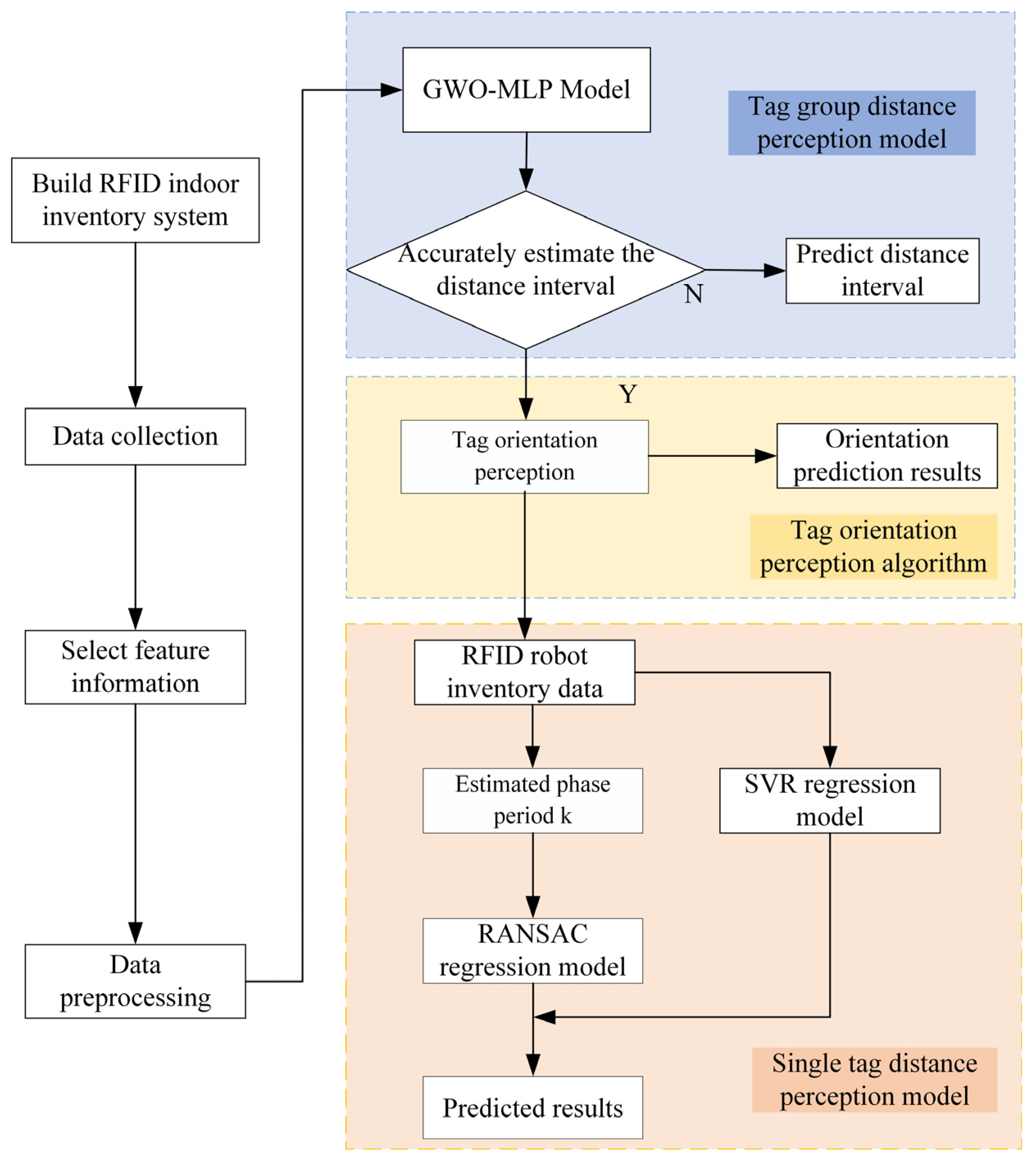
3. RFID Tag Position Perception Method and Theoretical Algorithm

In indoor scenarios such as libraries, warehouses, and hospitals, the deployment of RFID tags is highly dense. However, challenges such as the presence of numerous obstacles, severe multipath effects, and uneven field strength distribution make it challenging to perform single–tag localization. This paper proposes a novel method for indoor tag positioning perception, which consists of three parts: tag group distance perception, tag group orientation prediction, and single–tag position perception. The group distance perception utilizes the GWO–MLP neural network classification model to classify the distance range of the tag group based on the RSSI and SoI features and estimate the distance of the tag group. If the distance and orientation of a specific tag are further required, it can be determined whether the distance between the tag and its tag group meets the conditions for close–range perception. If so, the tag group can be divided into multiple sub–tag groups using a group orientation perception algorithm, and the orientation of each sub–tag group can be outputted. Then, by combining the RSSI and phase information of the tag, precise positioning of the single tag can be achieved. Figure 1 illustrates the flowchart of RFID tag position perception.

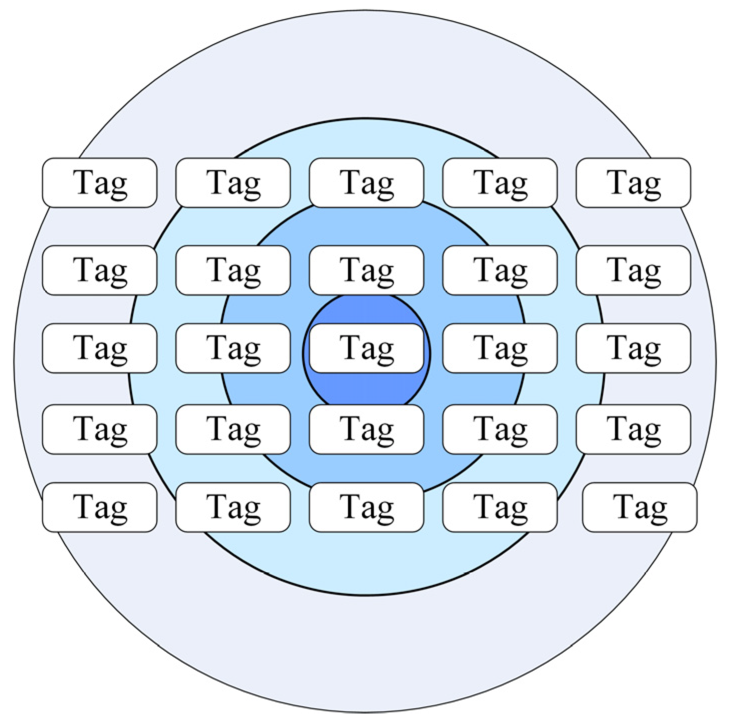
3.1. Basic Theory of Distance Perception for RFID Tag Groups

In dense indoor tag deployment scenarios, factors such as mutual interference between tags and indoor multipath effects can result in significant errors in individual tag positioning. Increasing the accuracy of localization would also increase the cost of the system. However, not all practical applications require high–precision positioning. Therefore, this paper proposes a tag group distance perception method to reduce the complexity and computational cost of system deployment and quickly and effectively predict the distribution of indoor RFID tag groups.

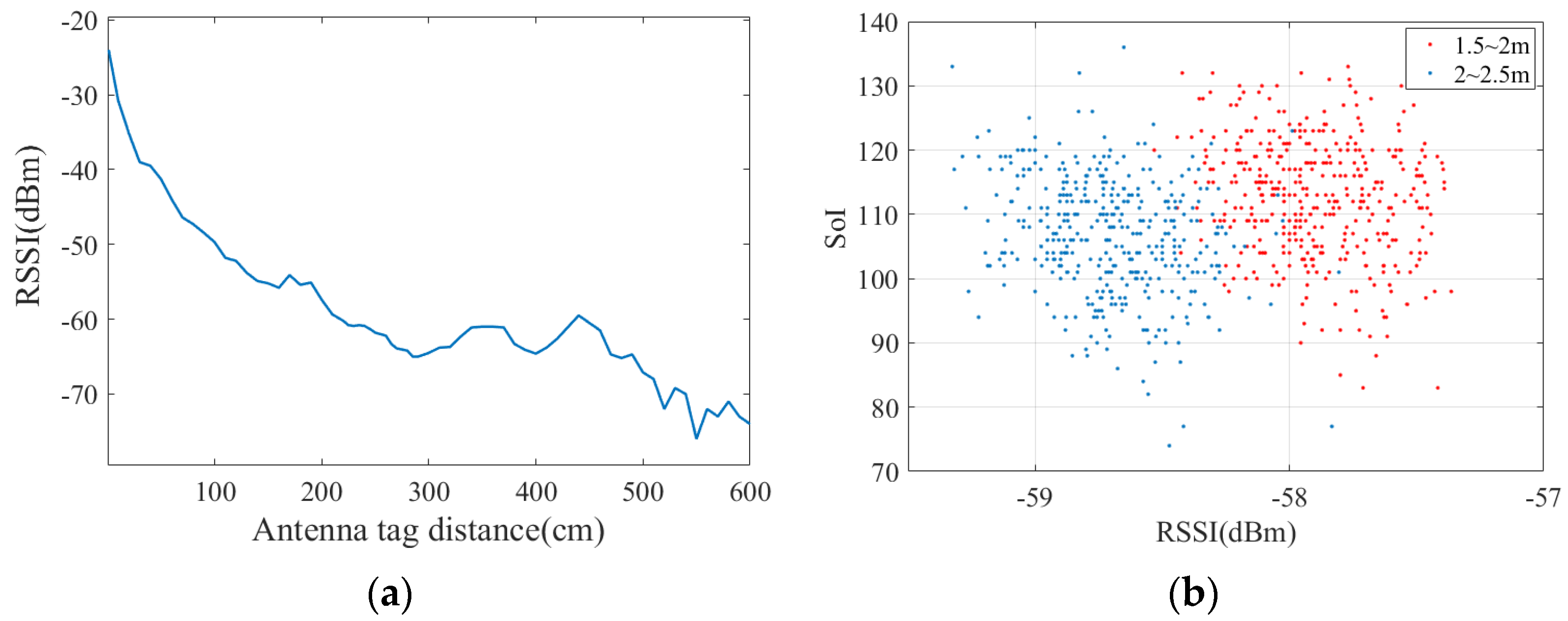
3.1.1. Combining RSSI and SoI for Distance Prediction

The working principle of the UHF RFID system is based on backscatter, where radio waves are transmitted from the reader to the tag and reflected to the reader by the tag. Equation (1) is derived based on the Friis equation [21], which provides the relationship between the received signal power and the distance between the reader antenna and the tag. The received power is converted to RSSI.

$$\left\{\begin{array}{c}Pr=Pt{(GtGr)}^2{(\frac{\lambda }{4\pi d})}^4\delta \\ P=\frac{Pr}{1mW}\\ RSSI=10\lg P\end{array}\right.$$

(1)

In Equation (1), $\lambda$ is the wavelength, $\delta$ is the attenuation coefficient, $d$ is the distance between the reader antenna and the tag, $PT$ represents the transmitting power of the reader, $Gt$ is the gain of the reader antenna, and $Gr$ is the gain of the tag antenna. Therefore, the position of the tag can be estimated by using RSSI.

Due to the complexity of the environment, multipath effects such as refraction, scattering, and diffraction can all influence the RSSI of the tag. As shown in Figure 2a, there is no one–to–one mapping relationship between RSSI and distance. Therefore, this paper introduces the SoI feature information to be combined with RSSI for distance prediction in tag groups. However, as shown in Figure 2b, the RSSI and SoI data samples in each distance interval are close and not linearly separable. The GWO–MLP algorithm is suitable for dealing with nonlinear problems. Through the multi–layer perceptron structure of the neural network, it can effectively fit nonlinear functions and possess strong generalization ability. Therefore, in this paper, the GWO–MLP algorithm is used to implement distance interval classification for tag groups.

3.1.2. GWO–MLP Algorithm

1.

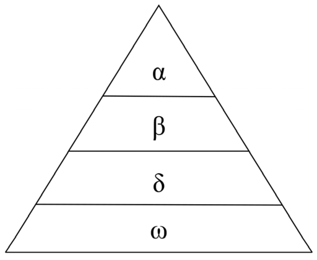
Grey Wolf Optimizer Algorithm

Grey Wolf Optimizer (GWO) [22] is an emerging and efficient swarm intelligence optimization algorithm inspired by the hunting behavior of grey wolf packs. GWO has the advantages of a simple structure, few adjustable parameters, and strong convergence.

The GWO defines the first ranked one as α wolves, which is the head wolf and will lead the movement of the pack, the second echelon as β wolves, the third echelon as δ wolves, who will assist α wolves, and the rest as ω wolves, as shown in Figure 3, by arranging the fitness values of individuals in the population in descending order. The coordinates of the α wolf represent the optimal solution.

2.

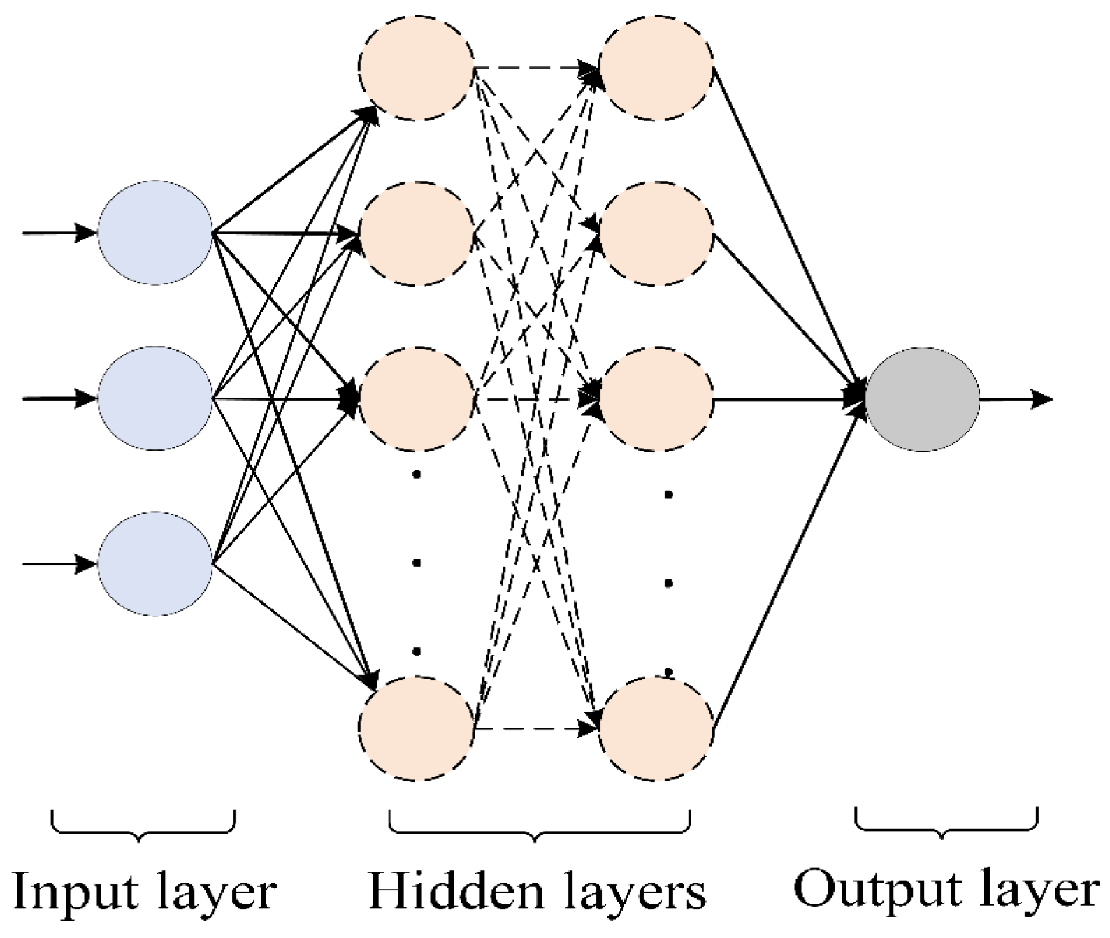
Multilayer Perception Machine Neural Network Model

Multilayer Perception (MLP) [23,24] is a kind of forward neural network with deep learning capability, which contains a large number of neurons in a multilayer network that can map a set of input vectors to a group of output vectors. MLP is generally three or more layers, and its model is shown in Figure 4.

MLP model propagation equation:

$$z_{ij}^l={\displaystyle {\sum }_j{W}_{ij}^l}·x_{ij}^{l-1}+b_j^l$$

(2)

$$y_i^{l+1}=f(z_{ij}^l)$$

(3)

where $x_{ij}^l$ is the input of the first layer, $W_{ij}^l$ and $b_j^l$ are the weights and biases of the layer neurons, respectively, $z_{ij}$ is the computed result of the $l$ layer, $y_i^{l+1}$ is the output result of this layer, and $f(·)$ is the activation function. In non–linear multi–class tasks, the activation function $softmax$ is typically used, and its expression is as follows:

$$softmax(x)=\frac{exp(x_i)}{{\displaystyle {\sum }_{i}exp(x_i)}}$$

(4)

The weight vector $w$ and bias vector $b$ are determined by the training process of MLP, which uses the Gray Wolf algorithm to optimize the weights and biases of the MLP model to improve the classification accuracy of the MLP model in the later stages.

3.1.3. Grey Wolf Optimization–Based MLP Multi–Classification Model

As an optimization algorithm, GWO optimizes the weights, biases, number of hidden layers, number of neurons per layer, and learning rate of each neural network in the MLP model. This generation’s α, β, and δ wolves are selected based on the fitness function values. GWO repeatedly iterates until it meets the required stopping conditions, and the optimal solution output is the selected α wolf. Then, the optimal solution of each parameter is extracted from the position of the α wolf and allocated to the MLP model for training. The GWO–MLP algorithm combines global search and local optimization capabilities, allowing it to find optimal solutions in a relatively short period. This makes it suitable for use in mobile scenarios.

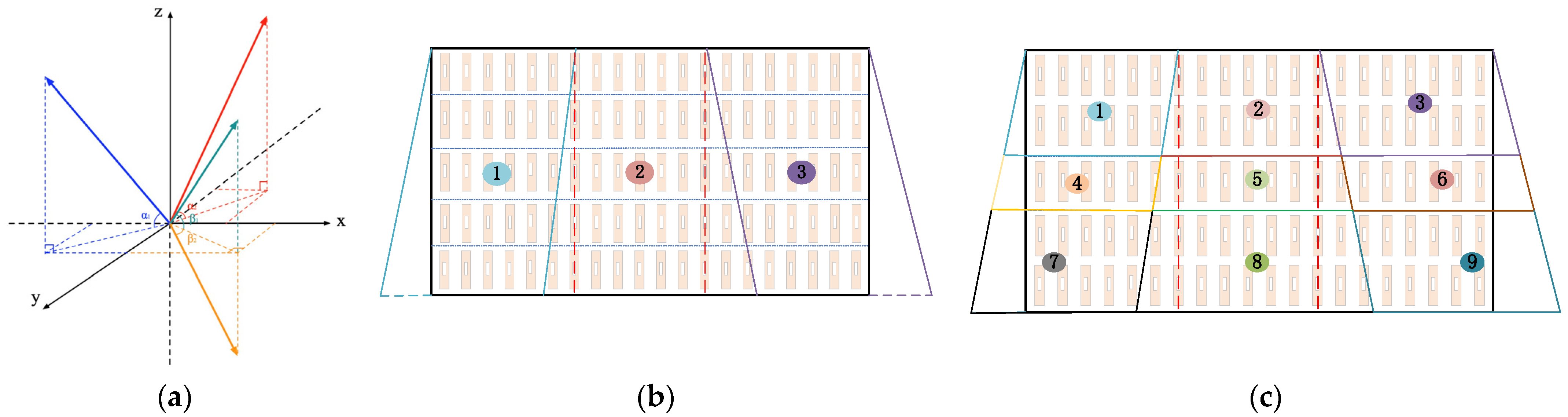
3.2. RFID Tag Orientation Perception Base Theory

The distance perception model for tag groups described in Section 4.4 is based on an archive shelve as a tag group for distance perception. However, at close–distance, the estimated distance range of the tags is too broad to meet the accuracy requirements. To address this issue, this paper proposes a tag group orientation prediction algorithm that can refine the tag groups into several sub–tag groups and effectively output the specific orientations of each sub–tag group. This not only improves the accuracy of the tag group position perception, but also enhances the applicability and engineering value of the model in practical applications.

Since passive RFID tags need to receive the energy emitted by the reader to activate themselves to transmit information, the angle between the direction of radiation reaching the tag from the reader’s antenna and the plane of the tag affects the tag’s identification performance. In theory, when the radiation direction is perpendicular to the tag plane, with a 90° angle, the recognition performance is optimal. As the angle decreases, the recognition performance decreases. Additionally, the RF electromagnetic waves emitted by the RFID antenna diverge in a spherical or conical shape. Theoretically, the reading range projected onto a plane should form a circular area, with the center of the reader’s recognition area having the highest energy density. As the area expands outward, the energy density gradually decreases, as shown in Figure 5.

Based on the above two points, it can be concluded that when the reader antenna is aligned horizontally and vertically with the center tag in the archive shelve, the energy density is highest at the center of the reader’s recognition area, which is also the center of the archive shelve. The antenna radiation direction is perpendicular to the tag plane, with an angle close to 90 degrees. In this region, the tags return bigger RSSI values. As the area expands outward from the center of the archive shelve, both the energy density and the antenna radiation angle decrease, resulting in a gradual decrease in the RSSI values returned by the tags.

The proposed algorithm for tag group orientation perception in this paper is based on changing the center region of the antenna scanning range and dividing the tag groups based on the RSSI variations returned by the tag group.

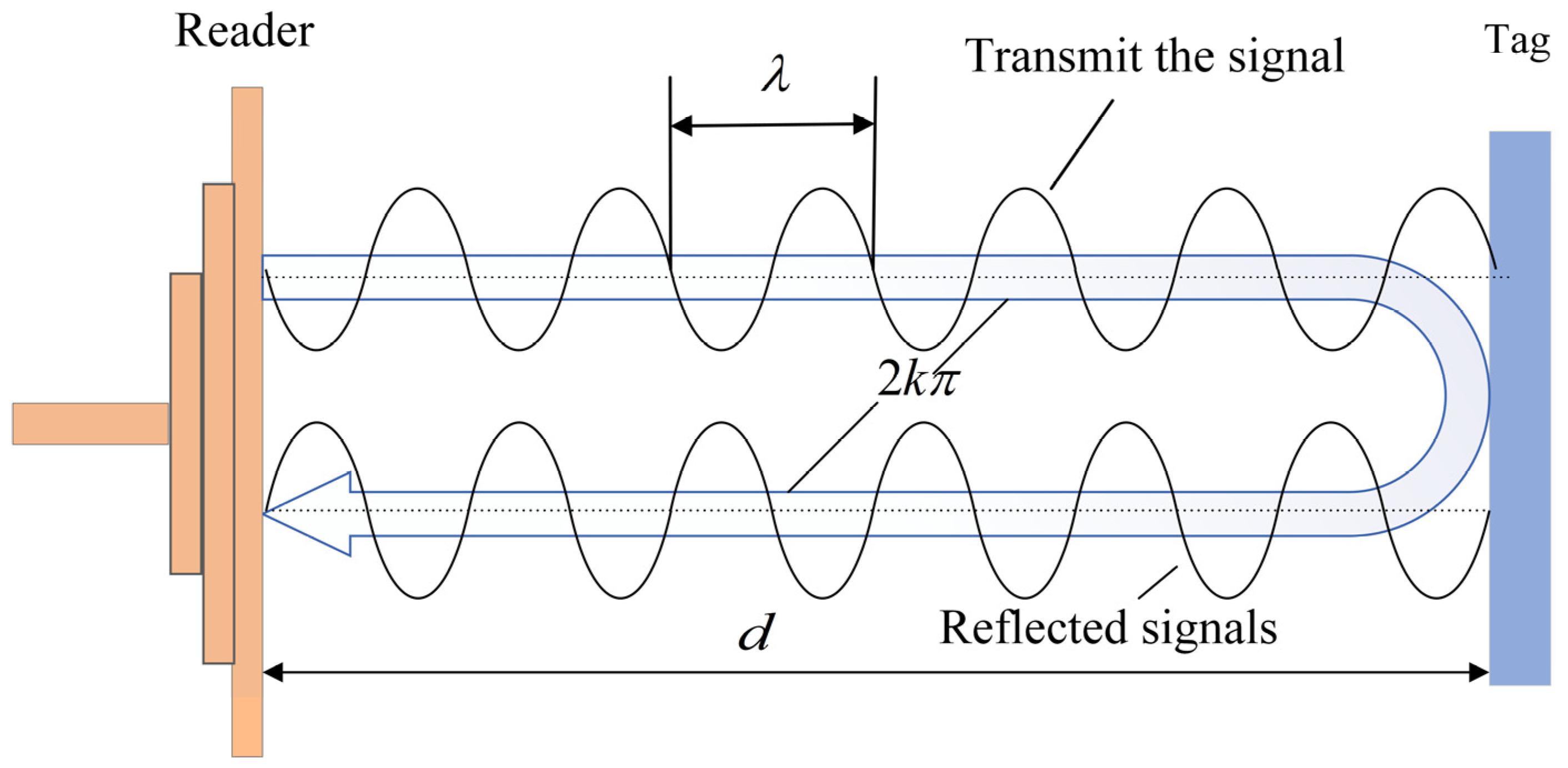
3.3. RFID Single Tag Precise Distance Perception Base Theory

The RFID wireless signal propagation model shows that the RSSI and phase returned by the tag are directly related to the signal propagation distance in space. Therefore, this paper combines the two channel characteristics of tag RSSI and phase to calculate the distance in reverse. Then, based on the predicted result of the tag group orientation, it outputs the single tag orientation and achieves single tag position perception.

3.3.1. RSSI Distance Perception Based on SVR Algorithm

This paper implements RSSI distance perception based on the Support Vector Regression (SVR) algorithm. The sample points in SVR ultimately belong to only one class, and the algorithm minimizes the total deviation of all sample points from the hyperplane [25]. In SVR, it is considered a correct prediction as long as the deviation between $f(x)$ and $y$ is not too large, and no loss calculation is necessary.

Equation (1) shows that RSSI and $d$ have a non–linear relationship, The paper uses the RBF kernel function, which only requires one parameter to be determined. In practical research, it has been found that using the RBF kernel function not only makes parameter optimization relatively simple but also results in better regression performance.

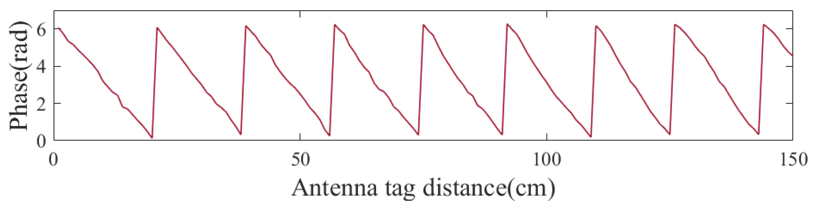
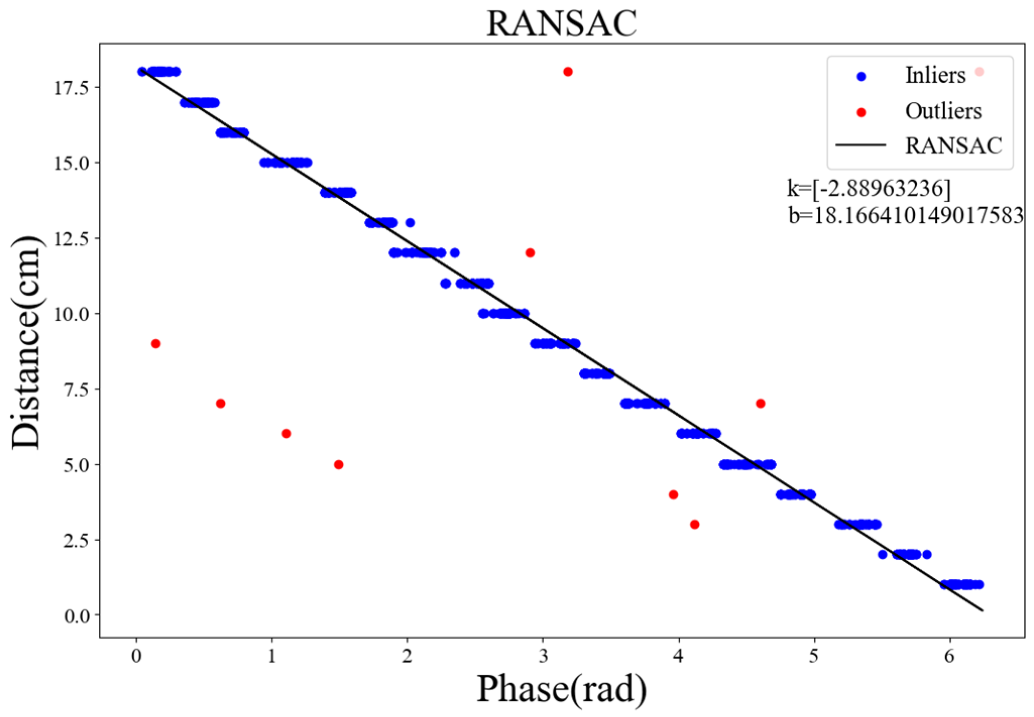
3.3.2. Phase Distance Perception Based on the RANSAC Algorithm

For an RF signal with a frequency of $f$, its wavelength is given by:

$$\lambda =\frac{\mathrm{c}}{f}$$

(5)

$c$ is electromagnetic wave speed; ImpinJ reader’s working frequency range is set to 902~928 MHz, according to the Equation (5) calculation, and its theoretical wavelength is 32.327~33.259 cm. The ImpinjR420 reader has a phase measurement accuracy of 0.0015 rad, which means that the phase is sufficient to perceive distance variations on the millimeter scale, offering the possibility of high–precision RFID localization [26]. Figure 6 shows the reader antenna and tag distance is $d$, RF signal total propagation distance is the antenna and tag distance twice, disregarding the phase shift caused by the hardware circuit of the reader and treating both the antenna and the tag as prime points [27,28,29], the phase is proportional to the propagation distance, and the ideal expression for the phase is given by:

$$\phi =\frac{2\pi }{\lambda }\times 2d$$

(6)

Equation (6) shows when the distance $d$ changes by half a wavelength ($\lambda /2$), the phase undergoes one cycle. By only changing the distance $d$ and obtaining the phase change curve as the distance $d$ gradually increases, it can be inferred that the phase change reflects the distance change to some extent.

Due to the linear relationship between phase and distance within $\lambda /2$, it is suitable for using a linear regression model, and due to the serious multipath interference in the indoor environment, even if the antenna and tag are close to each other, the measured phase data will still have unpredictable outliers. Outliers influence the general linear regression algorithm, and the regression coefficient estimation will be biased. In this paper, the RANSAC (Random Sample Consensus) [30] robust regression algorithm is used to solve the problem that the general linear regression is affected by outliers.

4. Indoor RFID Tag Position Perception Model Construction

This section will introduce the setup of experimental equipment and testing platform, and the establishment of the indoor RFID tag position perception model. A multi–tag testing platform for indoor UHF passive RFID will be built specifically for the proposed perception model.

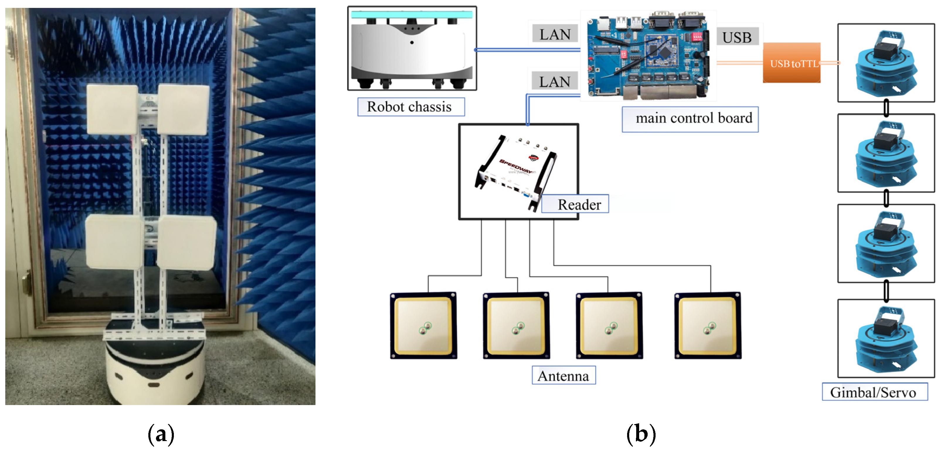
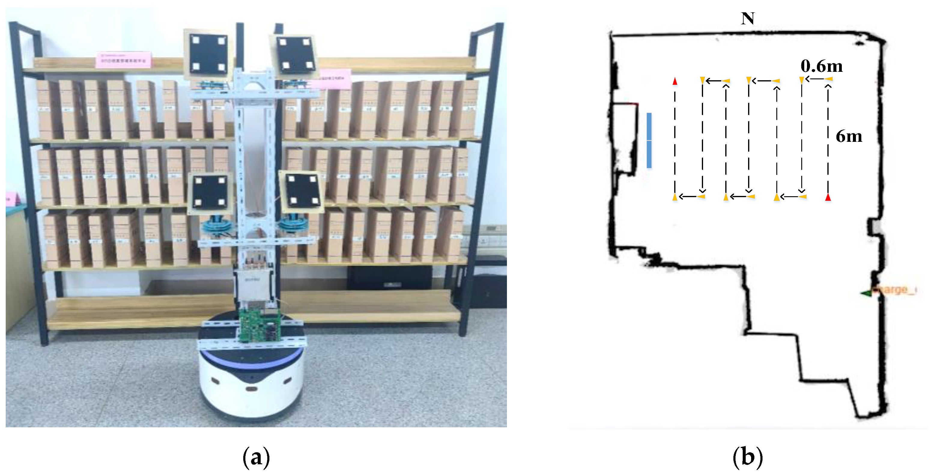
4.1. Testing Equipment

This paper combines mobile robots with UHF RFID systems to realize a UHF RFID robot inventory system. The system has the functions of cloud control, autonomous navigation movement, and omnidirectional antenna attitude control. Figure 7a shows the RFID robot, which is composed of a main control unit, a navigation robot unit, a UHF RFID system, and a gimbal unit. The main control unit is connected to the navigation robot and RFID reader through an Ethernet port, providing good computing power for robot control and real–time data analysis in mobile scenarios. The autonomous navigation robot cell is equipped with simultaneous localization and map building (SLAM) localization, cloud–based servo scheduling, etc. It can realize differential drive and active suspension and is equipped with hardware modules such as laser ranging sensors, RGBD depth cameras, ultrasonic ranging sensors, etc., so that it can easily realize all kinds of RFID inventory tasks in mobile scenarios. The gimbal unit is used to control the antenna attitude to improve system flexibility. In mobile scenarios, the inventory rate of tags in blind spots and dead corners is low. Mounted on a gimbal, the RFID reader antenna can freely rotate. Hence, the inventory efficiency is improved, and the occurrence of missed readings is reduced. The robot is powered by the chassis and equipped with four 9 dBi circularly polarized antennas. Figure 7b shows the hardware topology of the RFID robot.

The specific specifications of RFID system equipment readers, antennas, and tags installed in the RFID robot are shown in

Table 1. System equipment selection and performance specifications.

Type	Apparatus	Features
Reader	Impinj	Stable reading and writing performance
Antenna	9 dBi circular polarization reader antenna	Uniform waveform range
RFID tags	UHF 915 Mhz electronic tag	Anti–pollution and durable

.

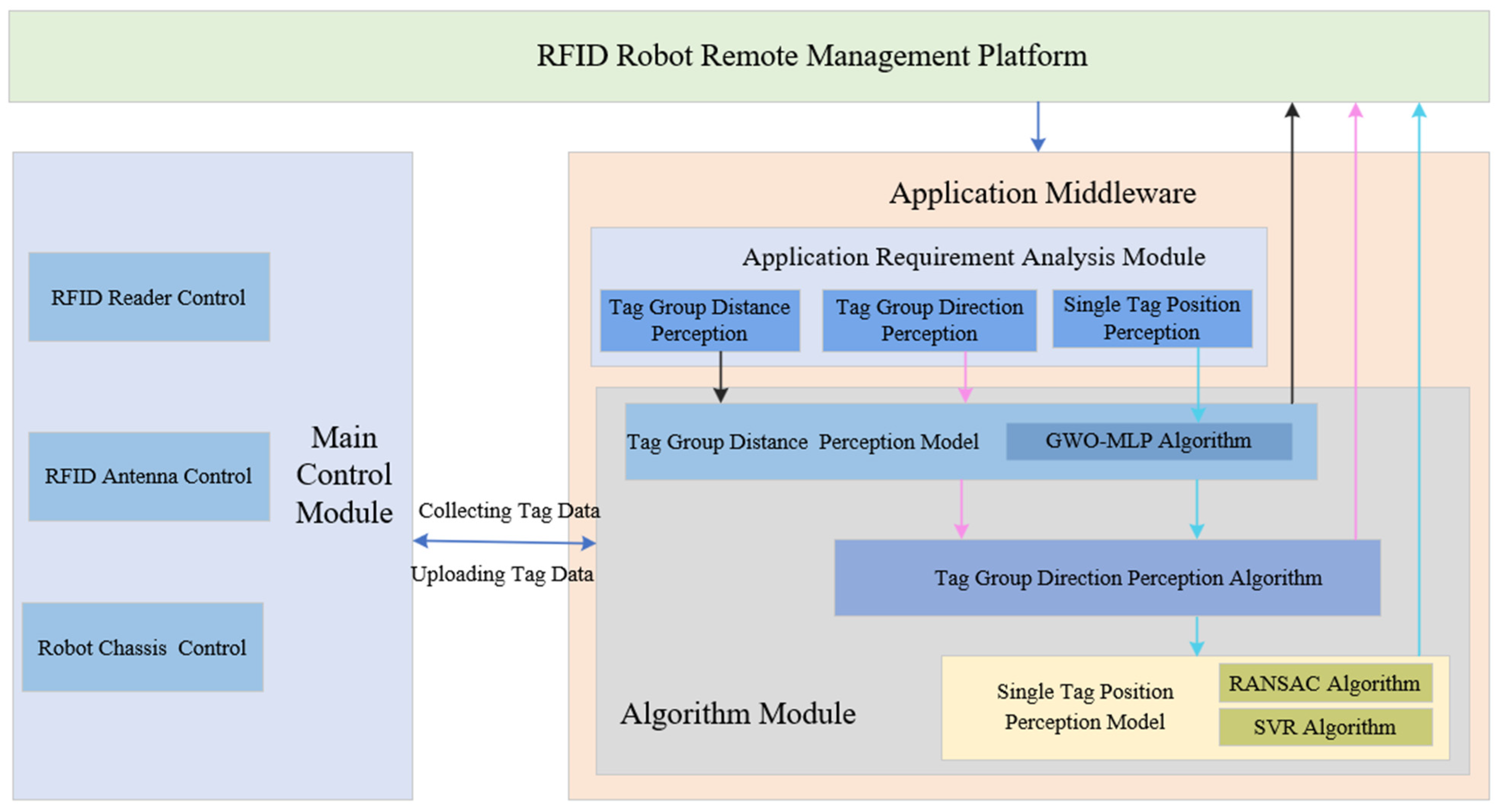
4.2. Software Architecture of RFID Robot Indoor Inventory System

The software architecture of the RFID robot indoor inventory system is shown in Figure 8, which consists of three parts: the application layer, the application middleware, and the main control module. Modules communicate with each other through TCP in synchronous or asynchronous mode to achieve control functions. The application layer implements remote activation of the robot inventory system and visualization of tag data analysis. The application middleware is responsible for intermediate data processing, event definition, and policy analysis. As shown in the figure, the event module is divided into tag group distance perception, tag group orientation perception, and single tag position perception events. By determining the user’s requirements, a specific event module is selected for execution, which then calls the main control module to control the reader, chassis, and antenna to obtain data for analysis and return the results to the application layer.

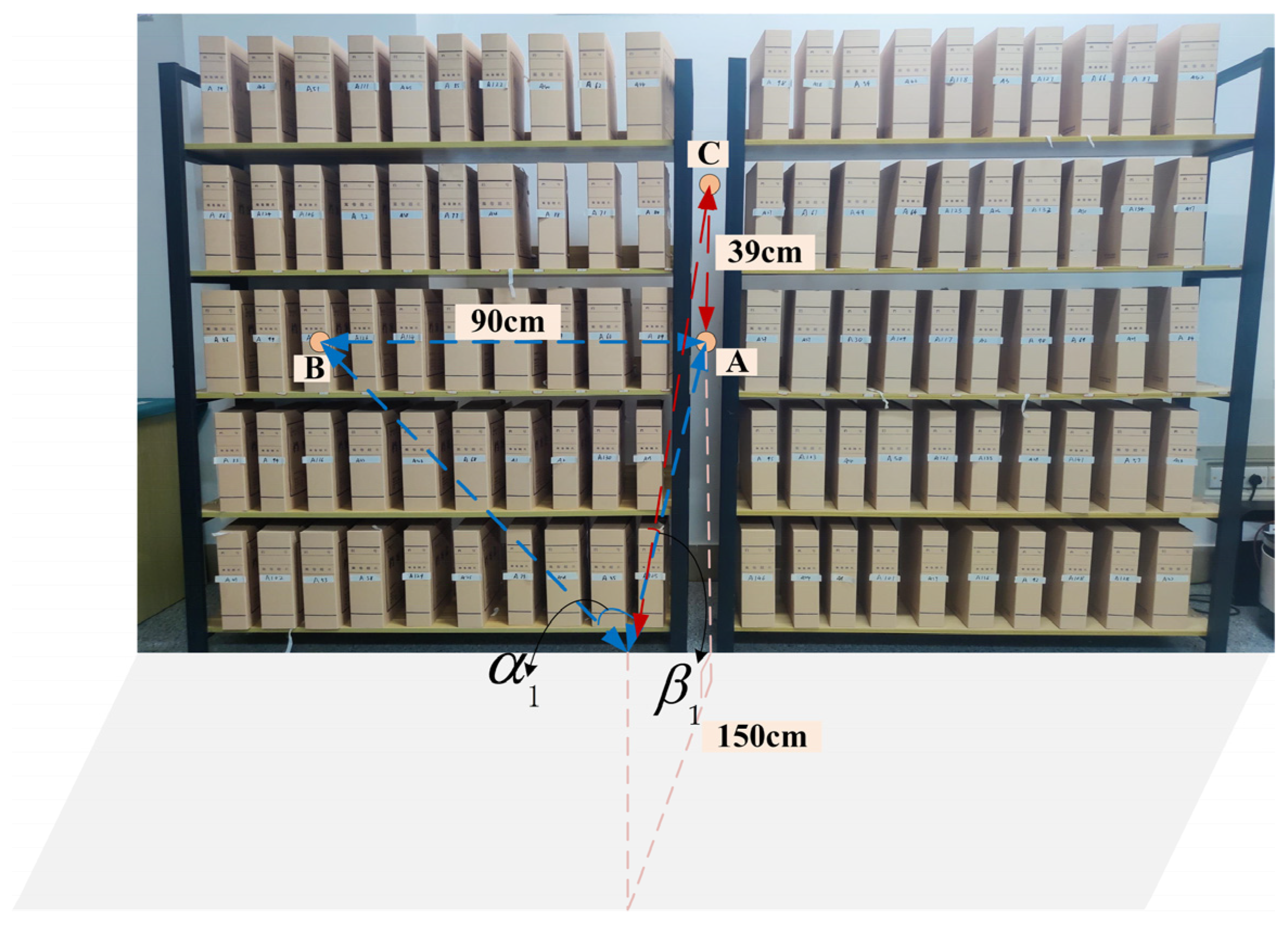
4.3. Testing Scenarios

The platform was built in a laboratory (L13 m ∗ W 8 m ∗ H 4 m) and arranged with two file shelves (L1.2 m ∗ H1.8 m), in five layers, with each layer evenly placed with RFID tags on the side of the file box; the test scenario is shown in Figure 9a. The robot collected RFID tags related information during the mobile inventory.

The map obtained by scanning with the instant localization and map construction (SLAM) function of the RFID robot chassis is shown in Figure 9b.

In Figure 9b, the blue dot position is equipped with an RFID tag archive box of two identical shelves, which can be regarded as a tag group in the mobile scene. The horizontal spacing of the two shelves is 0 m, and the number of tag deployments is 100. The red dot position in the figure is the starting point and termination position of the RFID robot, the yellow dot is the robot in the implementation of the tag inventory task needs to pass through the distance between the north and south points are 6 m, and the distance between the east and west points is 0.6 m. The robot scans each point in the room in an “S” type path. The test parameters are set as shown in

Table 2. Testing parameter settings.

Parameters	Parameter Value
Reader Power	27 dBm
Frequency	902~928 MHz
Data acquisition interval	10 s
Robot Speed	0.5 m/s
Inventory method	Asynchronous Inventory

. The RFID robot backend sends all the collected tag data to the middleware module.

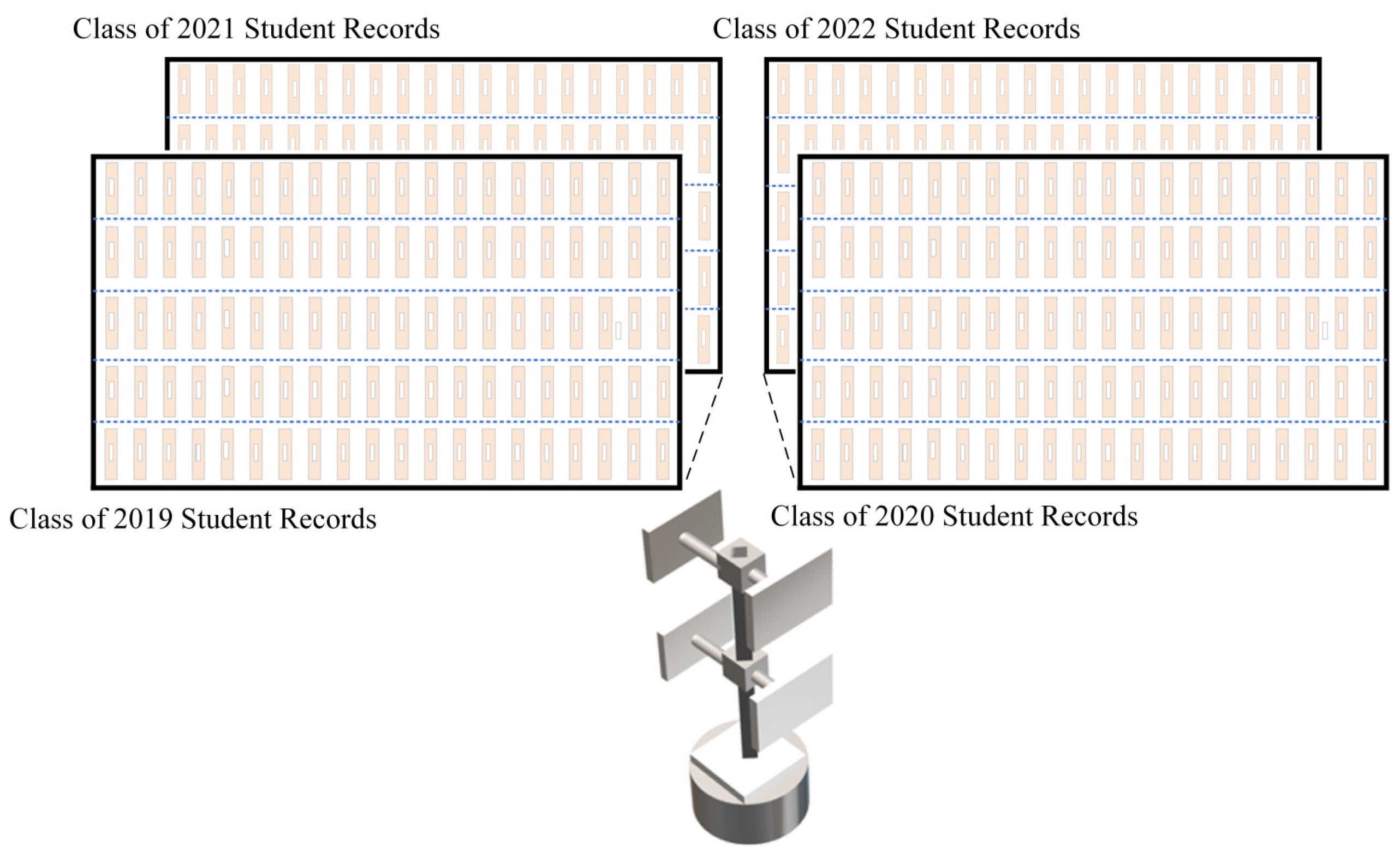
4.4. Tag Group Classification

In this paper, for the needs of unmanned warehouse parcel categorization, library book categorization, and archive management categorization, the tags attached to different parcels, books, or archives are categorized. Taking archive management as an example, as shown in Figure 10, four archive shelves are placed with different grades of student archive materials, and the respective category numbers are set in the EPC numbers of the archive tags on these four archive shelves, e.g., the category number in the EPC numbers of all tags for the student archives of the class of 2019 is set to 1. In the distance perception of the tag group, the tags are automatically classified into four tag groups based on the category numbers of the tags and the further distance perception of these four tag groups separately. This avoids the situation where the RFID robot considers all tags as one tag group, resulting in errors in tag distance perception.

4.5. Tag Group Distance Perception Model Building

Tag group distance perception builds a GWO–MLP model to classify the distance intervals based on two characteristic information: RSSI returned by the tag group and SoI. Figure 11 shows the flow chart of distance perception for the long–distance tag group.

4.5.1. Tag Group Distance Perception Data Collection

To perceive the horizontal distance between the tag group and the reader antenna, the horizontal distance between the antenna and the tag group is used as a decision attribute. In total, 50 tags are selected, the antenna power is 27 dBm, and the angle is orthogonal to the ground. The horizontal distance between the antenna and the tag group starts from 0.5 m to 6 m, and each time steps 0.5 m towards the far end horizontally. At each distance, 400 sets of data are tested, and the total number of data sets is 4800.

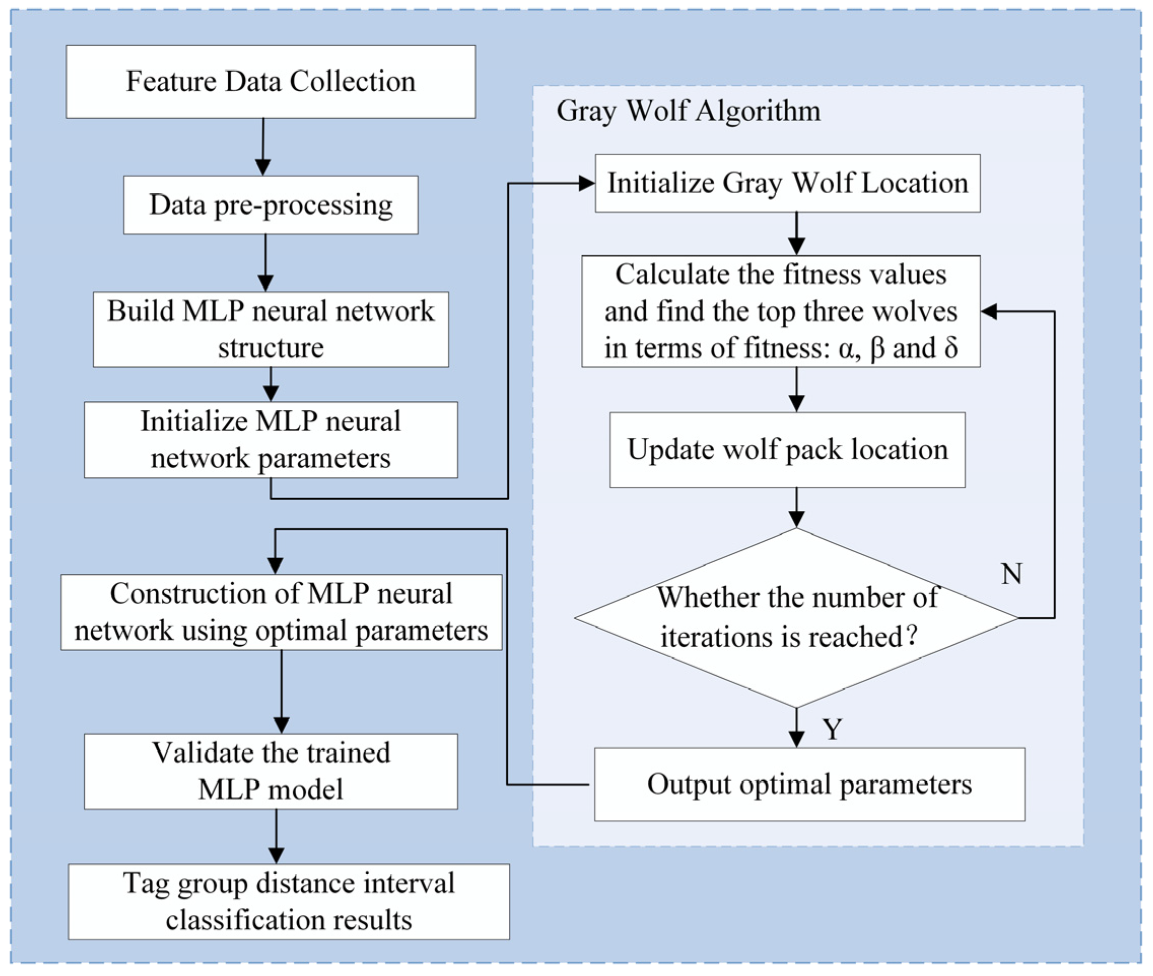
4.5.2. Establishment of GWO–MLP Model

Step 1: The collected data on RSSI and SoI are formed into a two–dimensional dataset with a size of 2400 × 2 as the conditional sample dataset, and normalized to obtain normalized values:

$$\overline{x}=\frac{x-x_{\min }}{x_{\max }-x_{\min }}$$

(7)

Step 2: The normalized dataset is divided into training, validation, and testing sets, and the MLP model structure is built. The number of neurons in the input and output layers of the MLP is determined based on the number of input parameters and output targets.

Step 3: GWO algorithm parameters are set, such as the maximum number of iterations, population size, optimization variable range, etc.

Step 4: The number of hidden layers, number of neurons in hidden layers, weight values, and bias values, as well as learning rate of the MLP neural network, are selected as the optimization variables, and the training set classification accuracy is used as the fitness function. Specifically, the fitness function formula is shown in Equation (8).

$$Fitness=\frac{n}{M}\times 100\%$$

(8)

where $n$ represents the number of incorrectly classified samples and M represents the total number of samples. The smaller the fitness value, the higher the classification accuracy of the optimized model.

Step 5: The hyperparameters of the MLP model are optimized by updating the α wolf, β wolf, and δ wolf positions by the fitness function.

Step 6: The trained GWO–MLP classification model is validated using test data, and the performance indexes of the MLP classification model on the test set, such as accuracy, precision, and recall, are calculated to evaluate the generalization ability and stability of the model.

4.5.3. GWO–MLP Neural Network Model Parameter Setting

The GWO–MLP model selects RSSI and SoI as its two input parameters, and the output variable is the distance category between the tag group and the reader antenna predicted by the GWO–MLP model. There are a total of 12 distance categories, ranging from 0 to 0.5 m, …, 5.5 to 6 m. Therefore, the number of neurons in the input and output layers in the MLP model is set to 2 and 12, respectively. The number of hidden layers is initially set to 1, and each hidden layer consists of 6 neurons. The maximum number of training sessions is limited to 50. The GWO algorithm uses 10 populations for iterations and sets the maximum number of iterations to 50.

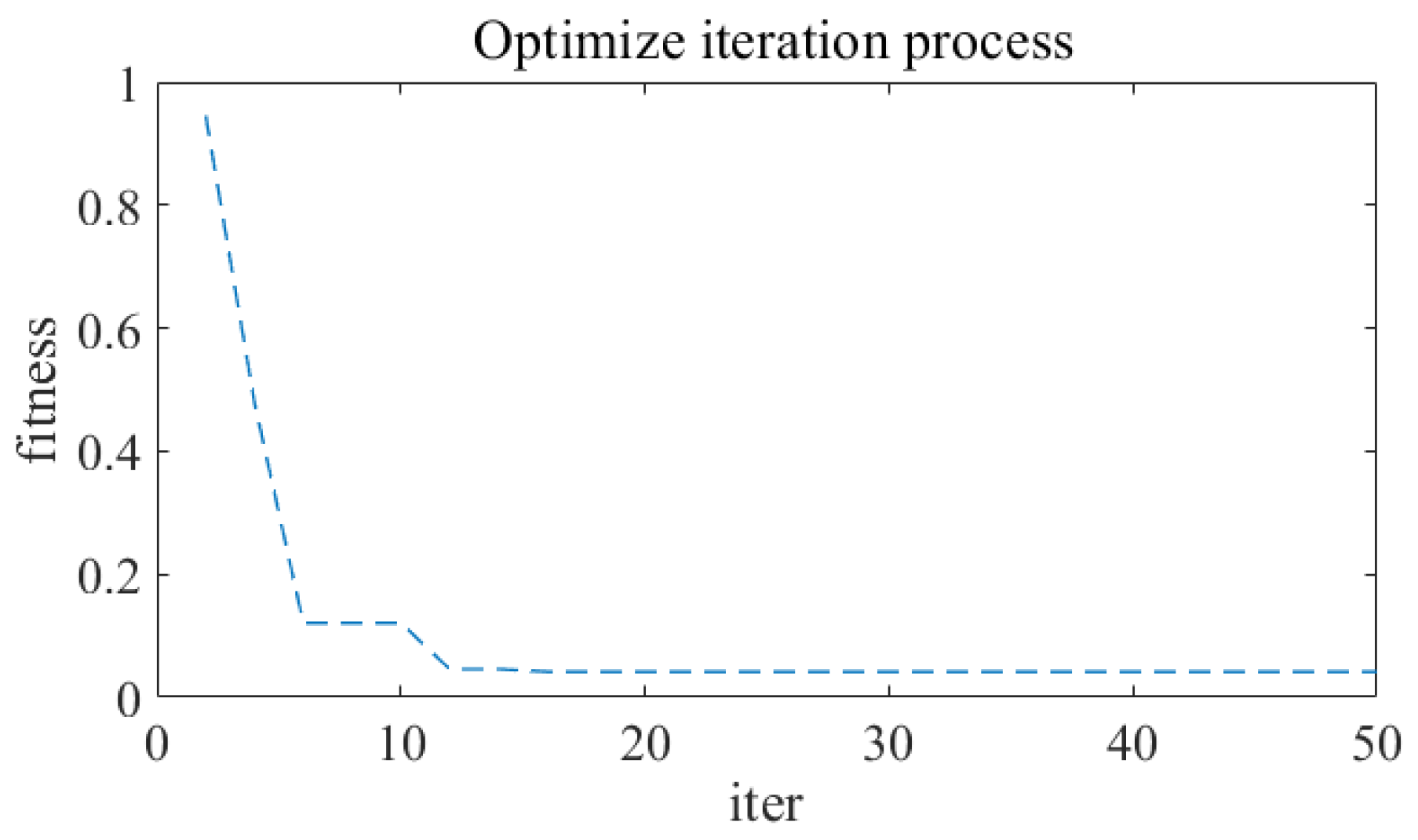
4.5.4. GWO–MLP Model Parameter Search Optimization

This paper utilizes the GWO optimization algorithm to search for the optimal parameters Figure 12 shows the adaptation curve of the GWO optimization algorithm, which indicates that the algorithm converges in less than 20 iterations, significantly less time compared to the cross–validation method. The optimal model has 2 hidden layers with 32 and 15 neurons, respectively, and a learning rate of 0.0012701.

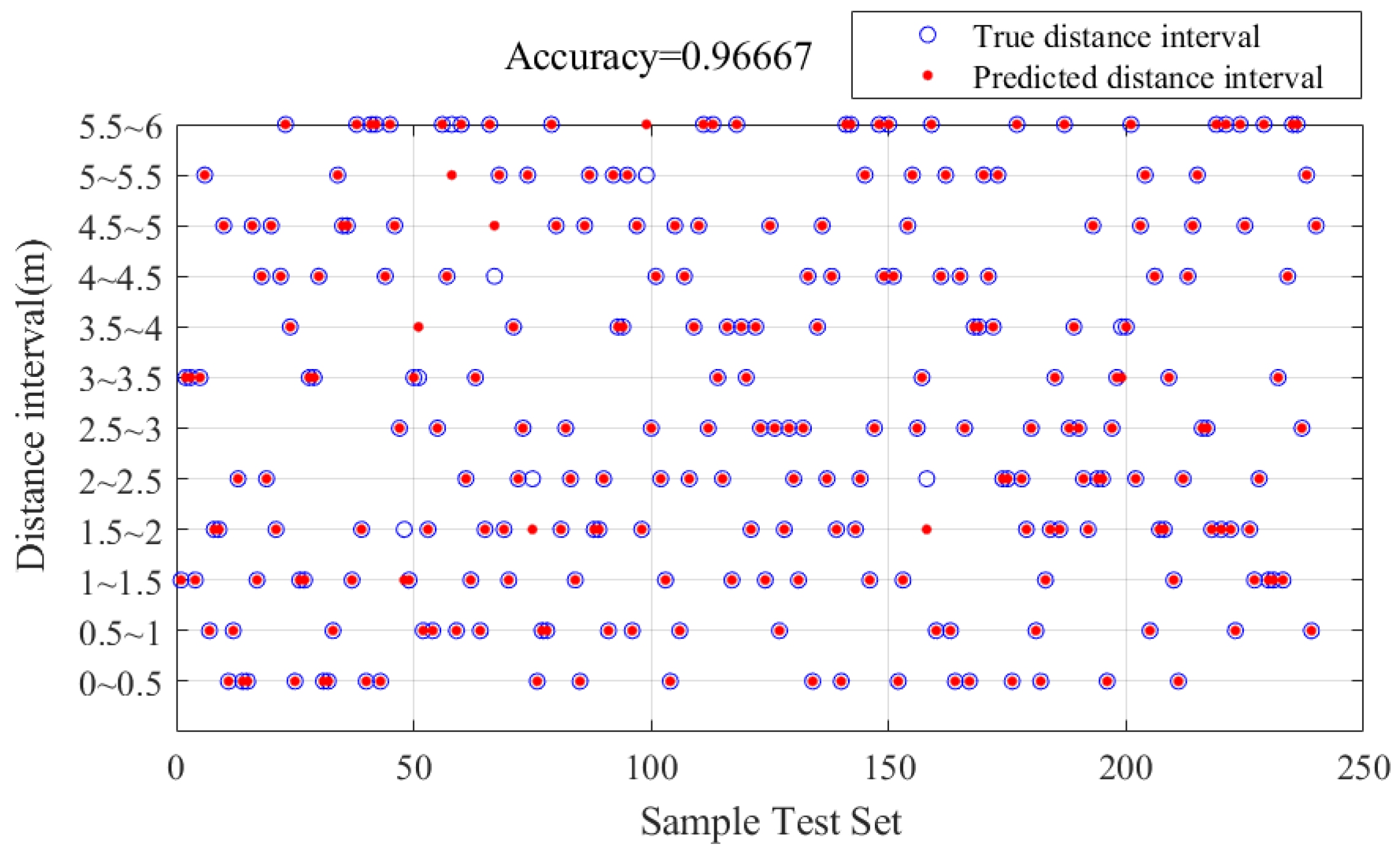
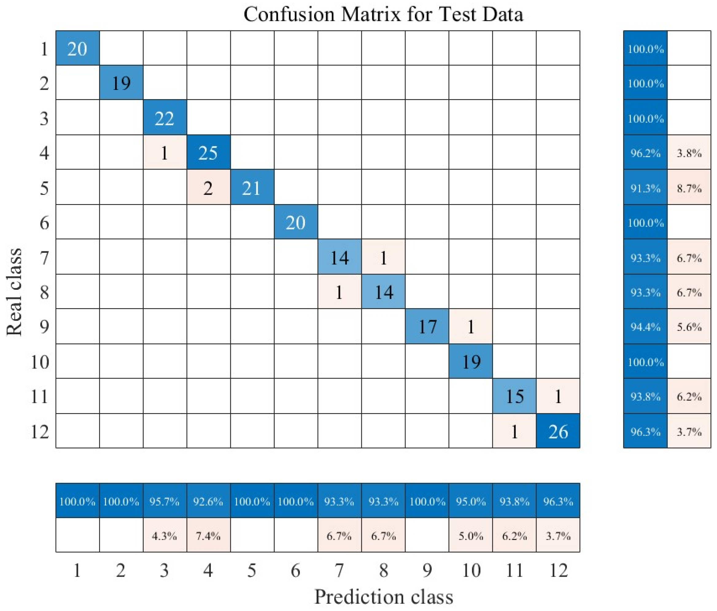
4.5.5. GWO–MLP Model Classification Results

The distribution of the classification results is presented in Figure 13. The model performed with an accuracy of 96.67%, which satisfies the accuracy requirements of RFID systems in mobile scenarios.

4.6. Tag Group Orientation Prediction Algorithm

The tag group orientation prediction algorithm proposed in this paper is to change the center region of the antenna scanning range, which leads to changes in the reader antenna radiation angle and energy density of the tags so that there are different changes in the RSSI of the tags in different regions, and then based on the tag group returned by the RSSI changes in the tag group segmentation. As shown in Figure 14a, the coordinate system takes the center point of the reader antenna as the origin. The initial direction of the RFID robot antenna is set to align vertically with the middle position of the archive shelve, and the original antenna angle is set to 0. Within a range of 1.5 m (According to Section 4.6), by adjusting the antenna’s angle, rotating it left by α1 degrees or right by α2 degrees, the tag group is divided into three sub–tag groups as shown in Figure 14b. Building upon the already divided three tag groups, further division is achieved by adjusting the antenna angle vertically, rotating it upwards by β1 degrees or downwards by β2 degrees, as shown in Figure 14c. This further divides the tag groups into nine parts. The antenna rotation angle values are calculated based on the actual length and height of the archive shelve.

This paper proposes tag group orientation prediction algorithms as shown in Algorithm 1 and Algorithm 2, with the algorithm parameters defined in

Table 3. Algorithm Parameter Definition.

Algorithm Parameters	Parameter Description
${\overline{RSSI}}_{{{}_i}_j}^{\eta }$	$i$$\eta$$\mathrm{for} \mathrm{the} j-th$ time (The RSSI of tags that have not been read is uniformly set to −80.)
$\Delta RSS{I}_i\left[\mathrm{j}\right]$	$i$$j$ times.
$\Delta R_i\left[\mathrm{j}\right]$	$i$
$\delta$	The threshold for determining whether the mean of the RSSI values of tags has changed.
$\epsilon$	The threshold for dividing tags from the main tag group
$R[\mathrm{a}]$	Sub–tag group with a quantity of “a” divided from the main tag group
$d$	The distance of tag group perception
$\left\{ALGORITHM 1(),({\alpha }_1,0,d_1)\right\}$	$\mathrm{The} \mathrm{tag} \mathrm{group} \mathrm{whose} \mathrm{coordinates} \mathrm{are} ({\alpha }_1,0,d_1)$ is further divided using the Algorithm

.

Algorithm 1. Tag group division sub–tag group algorithm

Input: $\delta$, $\epsilon$, $\eta$ ($\eta$: α1, α2, β1, β2) Output: $R[a]$

$\Delta RSS{I}_i[j]=[{\overline{RSSI}}_{{{}_i}_0}^{\eta }-{\overline{RSSI}}_{{{}_i}_0}^0,{\overline{RSSI}}_{{{}_i}_1}^{\eta }-{\overline{RSSI}}_{{{}_i}_1}^0,\dots \dots ,{\overline{RSSI}}_{{{}_i}_j}^{\eta }-{\overline{RSSI}}_{{}_{ij}}^0]$ $\Delta R_i\left[j]=\mathrm{sgn}\right(\Delta RSS{I}_i[j\left]\right)$ for $k=1$ to $j$ do     if $\Delta {\mathrm{RSSI}}_i[k]>\delta$        $\Delta R_i[k] =+1$; $k++$        $continue$      if $-\delta \le \Delta {\mathrm{RSSI}}_i[k]\le \delta$        $\Delta R_i[k] =0$; $k++$        $continue$      else $\Delta {\mathrm{RSSI}}_i[k]<-\delta$          $\Delta R_i[k] =-1$ for $n=1$ to $i$ do   if ${\displaystyle \sum _j\Delta R_n}>\epsilon$      $R[a]=n_{EPC}$; $a++$; $n++$    else      $n++$ if $a\le 0$     $Robot moving\to \eta$; $ALGORITHM 1$ else   return $R[a]$

Algorithm 2. Tag group orientation perception algorithm

Input: $d$, $\eta$ ($\eta$: α1, α2, β1, β2), $\delta$, $\epsilon$ Output: Coordinates of the sub–tag group

if $1.5<d<6$    return $(0,0,d)$ if $d\le 1.5$      $antenna angle:0\to {\alpha }_1$         $ALGORITHM 1(\delta ,\epsilon ,{\alpha }_1)\to ({\alpha }_1,0,d_1)$      $antenna angle:0\to {\alpha }_2$         $ALGORITHM 1(\delta ,\epsilon ,{\alpha }_2)\to ({\alpha }_2,0,d_2)$      $\left\{(0,0,d)-({\alpha }_1,0,d_1)-({\alpha }_2,0,d_2)\right\}\to (0,0,d_3)$      $antenna angle:0\to {\beta }_1$        $\left\{ALGORITHM 1(\delta ,\epsilon ,{\beta }_1),({\alpha }_1,0,d_1)\right\}\to ({\alpha }_1,{\beta }_1,d_{11})$        $\left\{ALGORITHM 1(\delta ,\epsilon ,{\beta }_1),({\alpha }_2,0,d_2)\right\}\to ({\alpha }_2,{\beta }_1,d_{21})$        $\left\{ALGORITHM 1(\delta ,\epsilon ,{\beta }_1),(0,0,d_3)\right\}\to (0,{\beta }_1,d_{31})$      $antenna angle:0\to {\beta }_2$         $\left\{ALGORITHM 1(\delta ,\epsilon ,{\beta }_2),({\alpha }_1,0,d_1)\right\}\to ({\alpha }_1,{\beta }_2,d_{12})$         $\left\{ALGORITHM 1(\delta ,\epsilon ,{\beta }_2),({\alpha }_2,0,d_2)\right\}\to ({\alpha }_2,{\beta }_2,d_{22})$         $\left\{ALGORITHM 1(\delta ,\epsilon ,{\beta }_2),(0,0,d_3)\right\}\to (0,{\beta }_2,d_{32})$    $\left\{({\alpha }_1,0,d_1)-({\alpha }_1,{\beta }_1,d_{11})-({\alpha }_1,{\beta }_2,d_{12})\right\}\to ({\alpha }_1,0,d_{13})$    $\left\{({\alpha }_2,0,d_2)-({\alpha }_2,{\beta }_1,d_{21})-({\alpha }_2,{\beta }_2,d_{22})\right\}\to ({\alpha }_2,0,d_{23})$    $\left\{(0,0,d_3)-(0,{\beta }_1,d_{31})-(0,{\beta }_2,d_{32})\right\}\to (0,0,d_{33})$ return $({\alpha }_1,{\beta }_1,d_{11})$, $({\alpha }_2,{\beta }_1,d_{21})$, $(0,{\beta }_1,d_{31})$, $({\alpha }_1,{\beta }_2,d_{12})$, $({\alpha }_2,{\beta }_2,d_{22})$, $(0,{\beta }_2,d_{32})$, $({\alpha }_1,0,d_{13})$, $({\alpha }_2,0,d_{23})$, $(0,0,d_{33})$

The threshold, antenna rotation angle, and distance of the tag group are input into Algorithm 2. Algorithm 2 calls Algorithm 1, which returns the sub–tag groups partitioned from the main tag group at that antenna angle. Algorithm 2then combines the orientation and distance of the sub–tag group to output the spatial position of the sub–tag group. In the algorithm, $({\alpha }_1,{\beta }_1,d_{11})$ represents the tag group in the $({\alpha }_1,{\beta }_1,d_{11})$ coordinate system, indicating that the tag group is located at an angle of ${\alpha }_1$ degrees to the left of the reader antenna, ${\beta }_1$ degrees above, and at a distance of $d_{11}$.

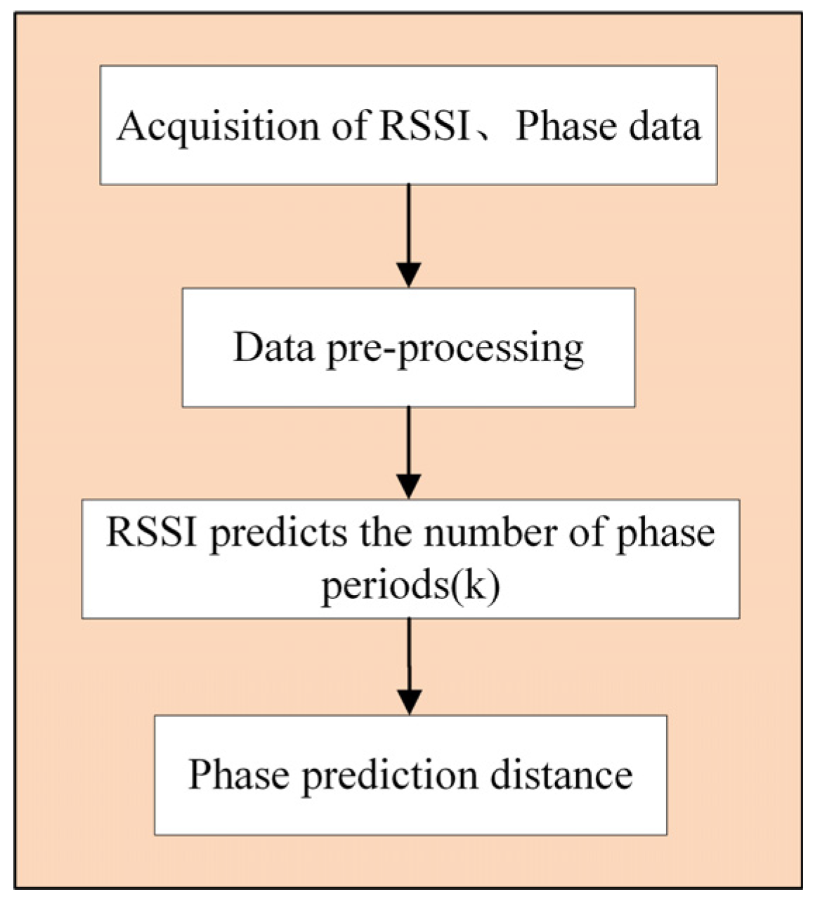
4.7. Single Tag Precise Distance Perception Model

After obtaining the orientation of each sub–tag group through the tag orientation prediction algorithm, if the specific position of a single tag in these tag groups is needed, further distance perception can be applied to that tag. The orientation of the tag in space is the same as the orientation of the tag group it belongs to.

The phase is more sensitive to distance perception and exhibits better robustness. Therefore, this paper focuses on single tag distance perception based on phase. However, the periodic variation of the phase value with $2\pi$, the reader can only output the main phase value within the range of $(0,2\pi )$ during the modulation and demodulation process. The output phase by the reader is identical at multiple distances, but in reality, there exist integer multiples of $2\pi$ between the phase values, i.e., $2k\pi$ ($k$ = 1, 2, …) of the whole cycle phase difference. How to judge the value of $k$ to avoid the problem of whole–period ambiguity is an important problem to be solved by the distance perception method based on the arrival phase.

Therefore, this paper proposes a method to determine the number of cycles $k$ experienced by the phase by using the property that RSSI decays with increasing distance. The flowchart for accurate perception of single–tag distance is shown in Figure 15.

As shown in Figure 9, indoor test scenario, the RSSI data returned by the tag directly in front of the reader antenna level are selected as the conditional sample, from 10 cm position to 5 m in steps of 10 cm each time. As shown in Figure 16, after the horizontal linear distance between the tag and the reader antenna exceeds 150 cm, the multipath effect has a greater impact on RSSI, and RSSI is no longer monotonically decreasing; it is impossible to accurately estimate the number of cycles $k$. Therefore, the range of single tag close–distance perception is 0–150 cm.

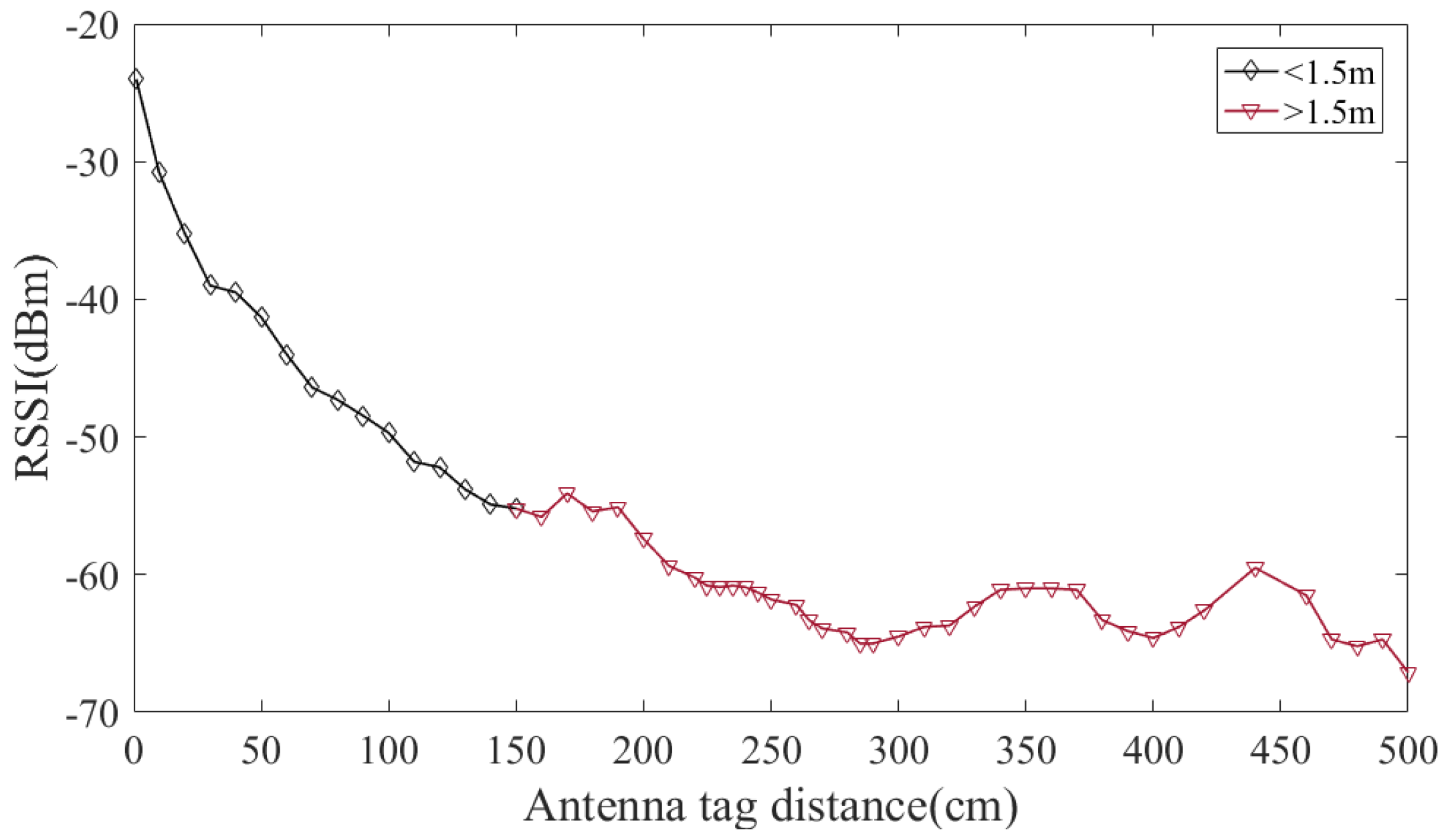
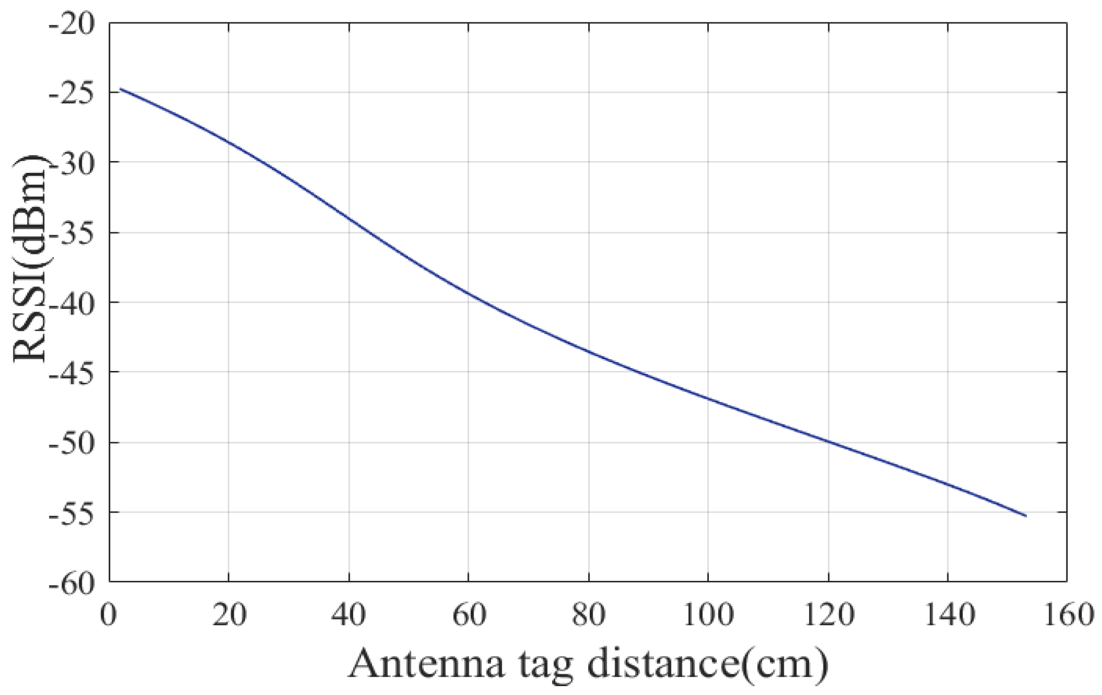
4.7.1. Data Collection and Pre–Processing

The phase and RSSI values returned by the single tag marked directly in front of the reader antenna level are collected as data samples, and the data are tested in steps of 1 cm from 1 cm to 150 cm each time, with 500 sets of data per distance, and the data set is 75,000 sets of data in total.

To reduce the data error, the collected RSSI and phase data sets need to be filtered, and since RSSI and phase are approximately normally distributed, Gaussian filtering is used in this paper. Gaussian filtering is used to remove interference values with significant errors from the raw data by calculating the average value of data within a high probability range to obtain the final data. Taking RSSI data filtering as an example, for a dataset containing N RSSI values, the Gaussian distribution is represented by Equations (9) and (10). Typically, the average value of RSSI within the range $[\mu -\sigma ,\mu +\sigma ]$ is chosen as the final RSSI value.

$$f(x)=\frac{1}{\sqrt{2\pi }\sigma }{e}^{-\frac{{(RSSI-\mu )}^2}{2\sigma }}$$

(9)

$$\mu =\frac{1}{N}{\displaystyle {\sum }_{j=1}^{N}RSS{I}_j},{\sigma }^2=\frac{1}{N-1}{{\displaystyle {\sum }_{i=1}^N(RSS{I}_j-\mu )}}^2$$

(10)

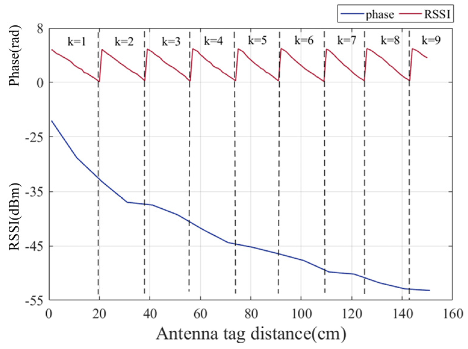
4.7.2. RSSI Estimates the Number of Cycles k Experienced by the Phase

RSSI estimate $k$ premise is required to determine the wavelength of the RF signal in the actual test, in the phase test will have the phase shift caused by the hardware circuit of the reader, so need to calibrate the phase, as shown in Figure 17 for the calibrated phase and distance change relationship graph, where half–wavelength of the actual test RF signal is 18 cm on average.

After obtaining the wavelength of the RF signal, as shown in Figure 18, the number of cycles $k$ of phase experience is determined by using the property that RSSI decays with increasing distance. The half–wavelength of the RF signal is used as the decision attribute, the RSSI data value after data pre–processing is used as the conditional attribute, and the RSSI data value is divided into nine categories according to the distance corresponding to each cycle of the phase, with each category representing the phase going through 1, 2, …, 9 cycles in turn.

4.7.3. Phase Prediction Distance

After determining the period $k$ of the phase, based on the characteristic that the linear relationship between phase and distance is valid only within $\lambda /2$, the RANSAC linear regression model is built within $\lambda /2$, and the phase data of each period are regressed to one period, with 70% of the data set as the training set and 30% as the test set, which are used to train the model and perform the evaluation of the generalization ability of the model, respectively. Before building the RANSAC algorithm model, two important parameters are the distance threshold and the number of iterations, which need to be set.

The distance threshold generally needs to be set empirically, and the phase value is more sensitive. In this regression model, the distance threshold is set to 0.8.

In traditional RANSAC implementation, the number of iterations or the inlier ratio needs to be predefined, which may result in poor regression performance. In this paper, the probability of “inliers” before establishing the model is unknown. An adaptive iteration method is used, and an infinite number of iterations is initially set. Then, when updating the estimated model parameters each time, the current “inlier” ratio is used as t to estimate the number of iterations. The formula for calculating the number of iterations is:

$$k=\frac{\log (1-P)}{\log (1-t^n)}$$

(11)

where P is the probability of obtaining a correct model from RANSAC. Figure 19 shows the RANSAC linear regression model.

The parameters evaluated in this model use the coefficient of determination (R²), and the R² of this model is 0.956, which is a better regression fit. The error distribution of the phase prediction distance within $\lambda /2$ is shown in Figure 20, where the maximum error is 0.6102 cm, and the average error is 0.2432 cm.

Assuming the predicted distance of the k–th phase cycle through the regression model is $d_k$, where $k$ is the number of phase cycles, then the antenna–to–tag distance can be expressed as:

$$d_{phase}=d_k+\frac{(k-1)\lambda }{2}$$

(12)

After verification, the maximum error $d_{phaseerror}$ of distance prediction based on phase in the single tag close–distance perception is 2.6102 cm, provided that the phase cycle number is correctly estimated using the RSSI. However, in complex indoor environments affected by multipath effects, the actual wavelength of the tested signal is uncertain. When estimating the phase cycle $k$ using the RSSI, the $\lambda /2$ is used as a decision attribute. As a result, the estimated phase experiences a cycle number $k$ error of plus or minus one. This leads to a larger error in distance prediction based on phase, up to $\lambda /2$.

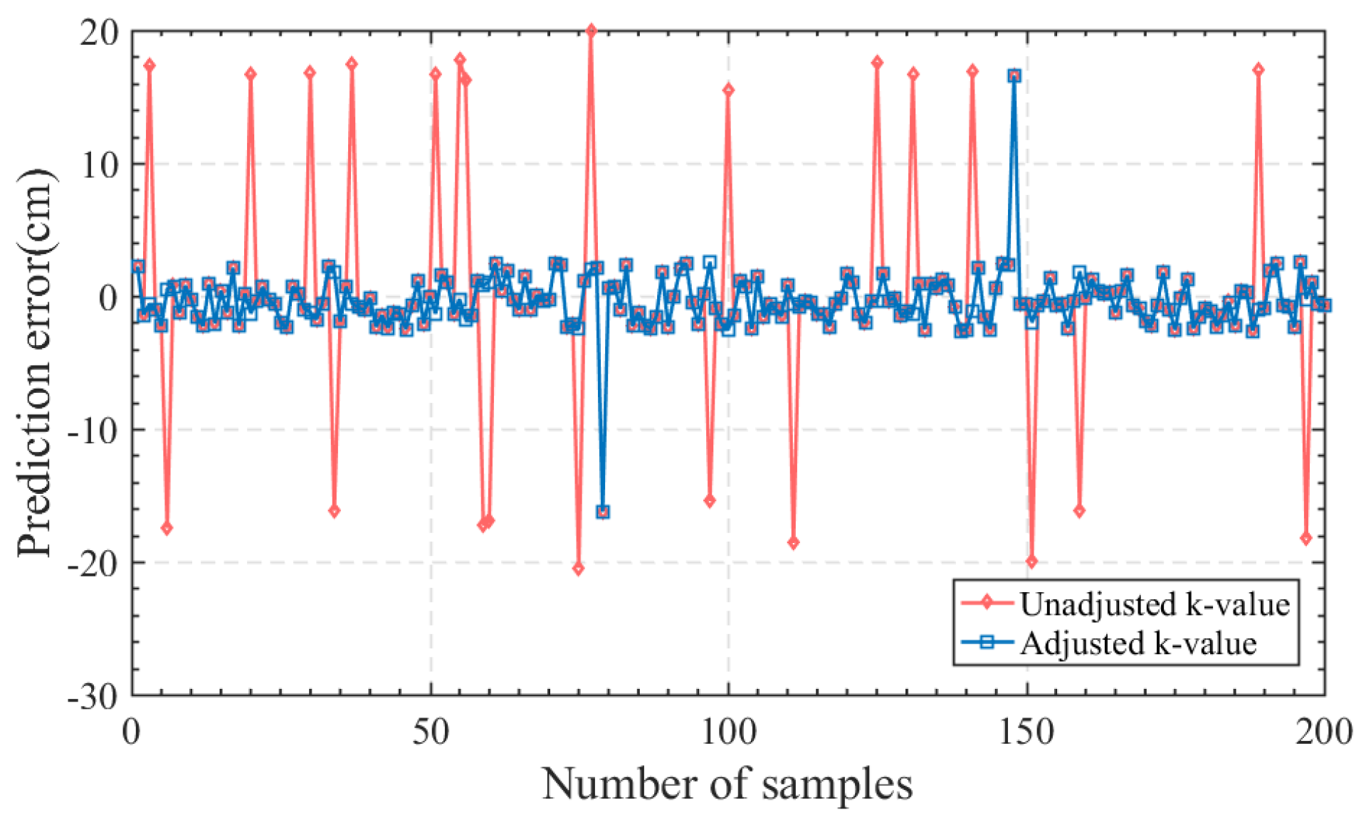
4.7.4. Single Tag Close–Distance Perception Model Improvement Algorithm

To solve the above–mentioned problem, this paper proposes the single tag close–distance perception model improvement algorithm, which introduces RSSI for close–distance joint perception and uses the distance predicted by RSSI as the reference distance $d_{RSSI}$, compares the reference distance $d_{RSSI}$ with the distance $d_{phase}$ predicted by phase, and determines whether $\left|d_{phase}-d_{RSSI}\right|$ is greater than $\lambda /2$, and if it is greater, the estimated phase period $k$ needs to be adjusted.

This paper uses the SVR algorithm to implement distance perception based on RSSI. As mentioned above, the range of single tag close–distance perception is limited to 0–150 cm, and the collected data are preprocessed before performing support vector machine regression analysis on it.

In the $\epsilon -SVR$ algorithm, the threshold $\epsilon$ is set to 0.01 (1 cm). As shown in Figure 16, RSSI and distance do not have a linear relationship. Therefore, the RBF kernel function is introduced to train a model for nonlinear data distribution and compute the prediction accuracy. Grid search and cross–validation are used to find the best parameters.

In total, 80% of the data are selected as the training set to train the SVR model, and 20% of the data are used as the test set to validate the trained model. The parameter optimization results show that the penalty coefficient $C=10$ and the kernel function parameter $g=10$.

Figure 21 shows the prediction results of the test set, with a root mean square error of 4.2394 cm. Figure 22 displays the distribution of the prediction distance error, with a maximum error of 11.4796 cm. When training the model, the tolerance for the offset of the set prediction distance is 1 cm, resulting in a maximum error of $d_{phaseerror}$ = 12.4796 cm for the RSSI prediction distance. The regression curve of RSSI and tag distance is presented in Figure 23.

The method to verify whether the period $k$ estimated by RSSI is correct is to determine whether the difference between the two distances $\left|d_{phase}-d_{RSSI}\right|$ is less than $\lambda /2$. If it is less than $\lambda /2$, it indicates that the estimated period $k$ is correct and no adjustment of $k$ is needed; if it is greater than $\lambda /2$, it indicates that $k$ needs to be adjusted. Furthermore, the size of $d_{RSSI}$ and $d_{phase}$ is determined. $d_{phase}>d_{RSSI}$ means that the estimated period is more than one period, and the original estimated $k$ needs to be subtracted by 1. $d_{phase}<d_{RSSI}$ means that the estimated period is less than one period, and the original estimated $k$ needs to be added by 1.

However, the above judgment method applies to the case where there is no error in the RSSI and phase prediction distance results. In the actual test, there are cases where the period number $k$ is incorrectly estimated but $\left|d_{phase}-d_{RSSI}\right|$ is also less than $\lambda /2$, so the judgment condition $\lambda /2$ is not applicable in the case of error. This paper chose $d_{phaseerror}$ + $d_{RSSIerror}$, as the maximum value of $\left|d_{phase}-d_{RSSI}\right|$ is $d_{phaseerror}$+$d_{RSSIerror}$ if the phase period $k$ is correctly estimated. If $\left|d_{phase}-d_{RSSI}\right|$ is greater than $d_{phaseerror}$+$d_{RSSIerror}$, it indicates that the phase period $k$ is wrong and the value of $k$ needs to be adjusted. The maximum error of RSSI and phase prediction distance is a limiting condition, and the probability is very small. $d_{phaseerror}$+$d_{RSSIerror}$ is a more appropriate condition for determination. The specific $k$–value adjustment algorithm is shown in Algorithm 3.

The input parameters of the algorithm are the pre–processed RSSI data, the calibrated phase value, and the average value of the half–wavelength in the actual test. The output is the adjusted phase period $k$, and the final predicted distanced $d$.

Algorithm 3. Single tag close–distance perception based on the k–value adjustment algorithm
Input: $RSSI,Phase, \frac{\lambda }{2}$ Output: $k,d$
RSSI classification model: Input: $RSSI,\frac{\lambda }{2}$        Output: $k_i$	SVR regression model:     Input: $RSSI$   Output: $d_{RSSI},d_{RSSIerror}$
RANSAC regression model:        Input: $k_i$    Output: $d_{k_i},d_{k_i}{}_{error}$      $d_{phase}=d_k{}_{{}_i}+\frac{(k-1)\lambda }{2},d_{phaseerror}$
If $\left|d_{phase}-d_{RSSI}\right|<d_{RSSIerror}+d_{phaseerror}$ then       return: $k=k_i,d=d_{phase}$   else      If $d_{phase}>d_{RSSI}$ then       return: $k=k_{i-1},d=d_{k_{i-1}}+\frac{(k_{i-1}-1)\lambda }{2}$     else        return: $k=k_{i+1},d=d_{k_{i+1}}+\frac{(k_{i+1}-1)\lambda }{2}$

5. Indoor RFID Tag Position Perception Model Validation

This section is to validate the algorithms established in Section 4, and the RFID robot inventory system conducts mobile inventory based on the environment and device parameters described in Section 4.2.

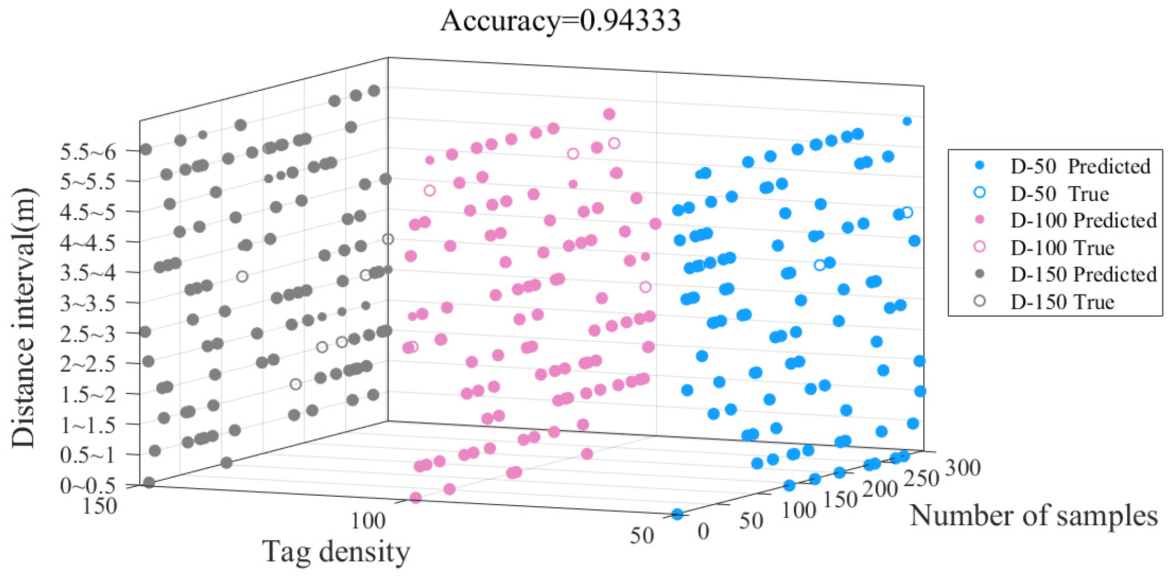
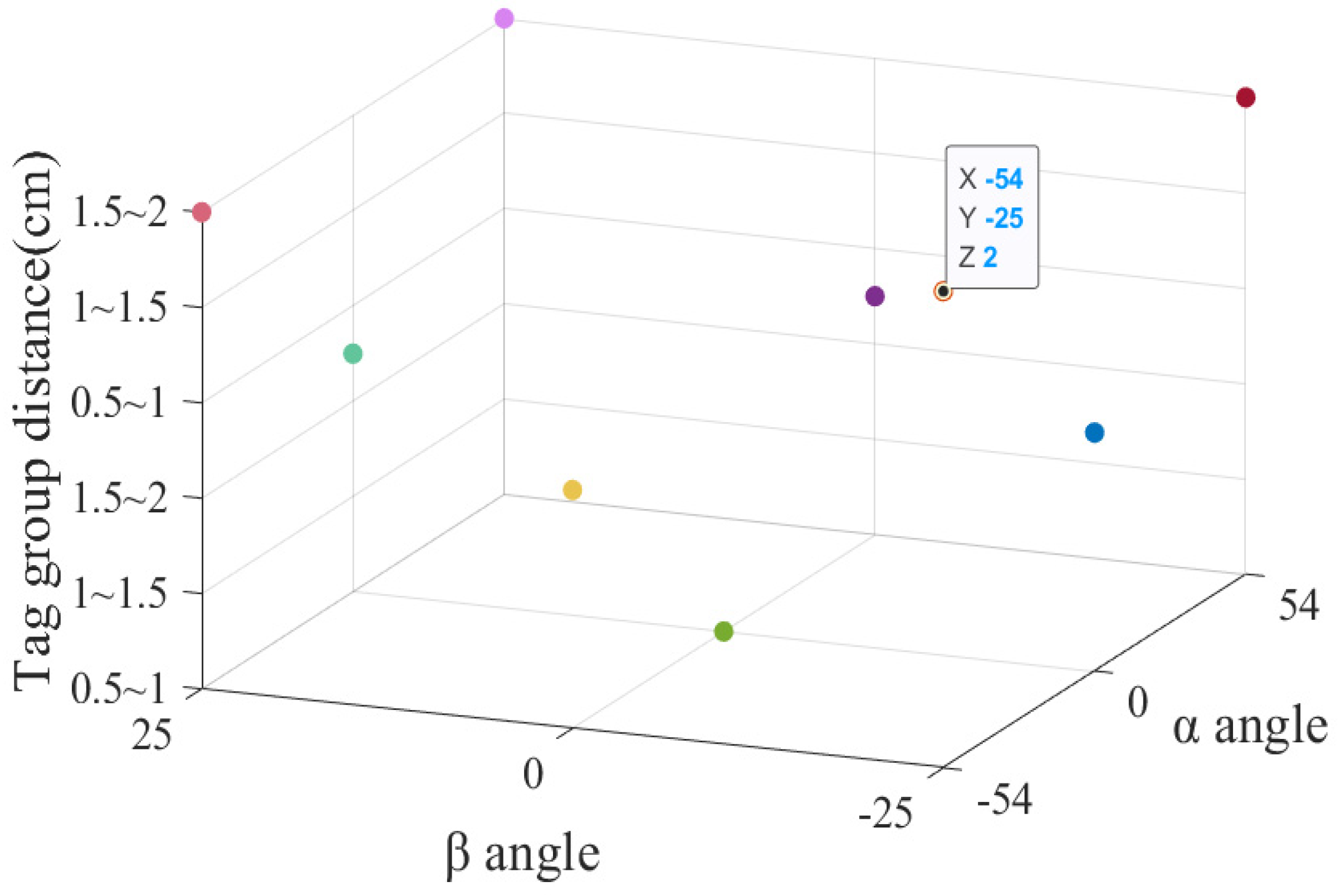
5.1. Tag Group Distance Perception Model Validation

To validate the performance of the tag distance perception algorithm under different tag densities, this study deployed testing scenarios with tag densities of 50, 100, and 150. Different sets of tag group feature information will be collected under each tag density, totaling 100 groups. The GWO–MLP classification algorithm will be applied to predict the results, which will be compared with the actual results. The prediction accuracy of the tag group distance perception model under different tag densities is shown in

Table 4. Prediction accuracy of distance interval of tag group in indoor environment.

Tag Group Density	Model Prediction Accuracy
50	97%
100	95%
150	91%
Average accuracy	94.333%

. The RFID tag group distance prediction results are shown in Figure 24. The distance perception classification accuracy decreases when the tag quantity is high, and the classification error is 9% when the tag group density is 150, but the average classification accuracy of the overall MLP model reaches 94.333%. If the robot’s moving speed is reduced to 0.2 m/s on this basis, the algorithm predicts that the classification error is reduced to 6%, which can better meet the needs of mobile scene engineering applications.

In this paper, a confusion matrix was constructed to evaluate the performance of the tag group distance perception model. Metrics such as accuracy, precision, recall, and F1 score were utilized for evaluation. The formula for calculating the F1 score is as follows.

$$F1=\frac{1}{12}{\displaystyle \sum _1^{12}2\ast \frac{Precision\ast Recall}{Precision+Recall}}$$

(13)

Figure 25 displays the confusion matrix of the GWO–MLP model with a tag density of 50. It can be observed from the figure that the precision and recall for each category are above 90%. Further calculation yields an overall F1 score of 96.57%, indicating that the GWO–MLP classification model exhibits high predictive accuracy and discriminative capability for various sample categories.

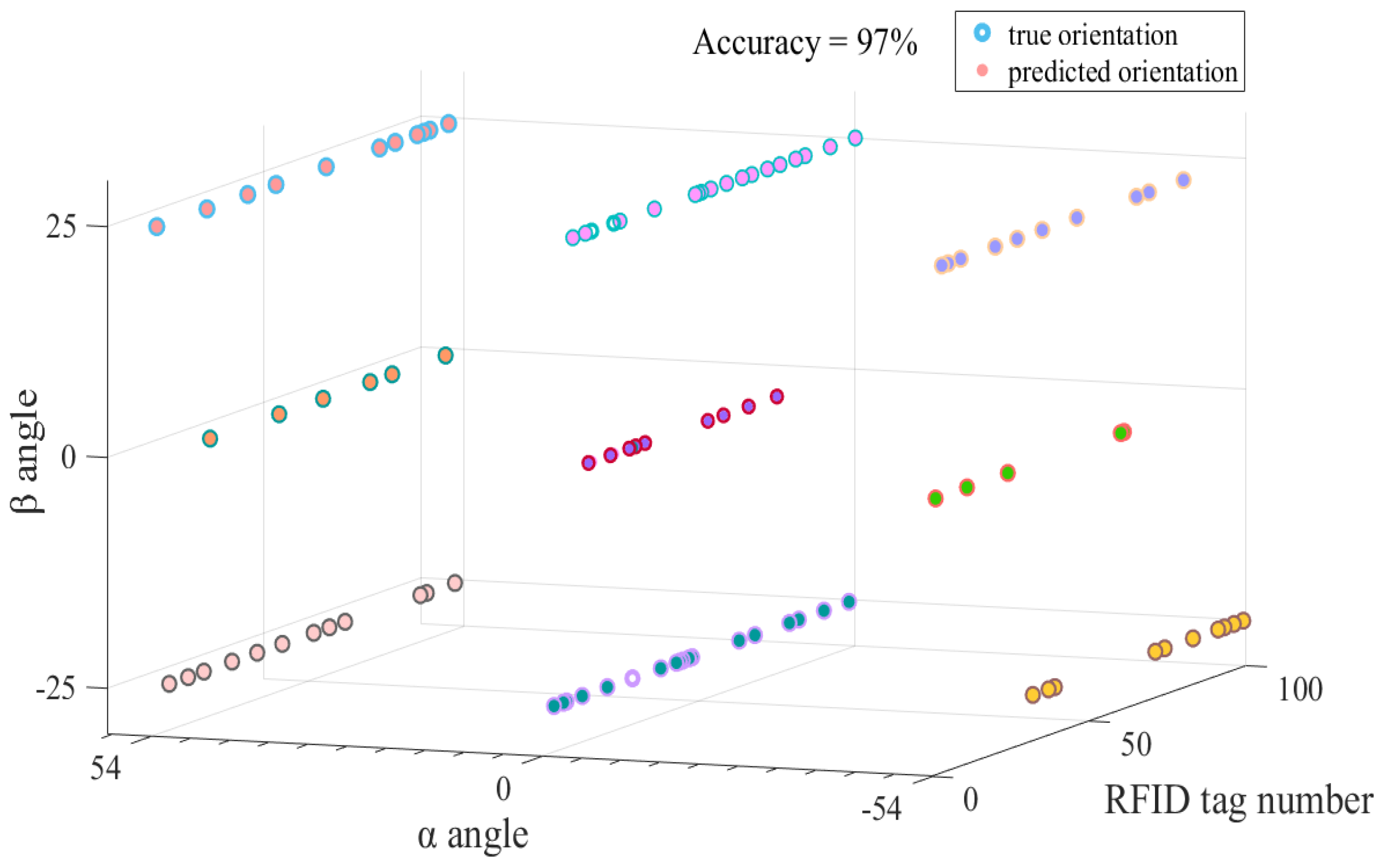
5.2. Tag Group Orientation Prediction Algorithm Verification

The RFID robot starts moving from a position 6 m away from the tag group, following the trajectory described in Section 4.2. During the movement, the RFID robot continuously measures the distance to the tag group. When $d<1.5$ m is satisfied, the tag group orientation estimation algorithm is executed.

1.

Antenna rotation angles ${\alpha }_1,{\alpha }_2,{\beta }_1,{\beta }_2$ values

Figure 26 shows the archive shelve used in the testing. Due to the small size of this archive shelve, two archive shelves are considered as one archive shelve in the orientation prediction algorithm. Point A in the figure represents the center position of the archive shelve, point B represents the predetermined position directly in front of the antenna when it is turned to the left, and point C represents the predetermined position directly in front of the antenna when it is turned upwards. The distance between points A and B is 90 cm, the distance between points A and C is 39 cm, and the horizontal distance from the archive shelve to the antenna is 150 cm. Therefore, the values of ${\alpha }_1,{\alpha }_2,{\beta }_1,{\beta }_2$ are given by the following equation:

$$\left\{\begin{array}{c}{\alpha }_1=\arctan \frac{90}{150}\approx 54°\\ {\beta }_1=\arctan \frac{39}{150}\approx 25°\end{array}\right.$$

(14)

Based on symmetry, ${\alpha }_2=-54°,{\beta }_2=-25°$.

2.

Threshold values for $\delta$ and $\epsilon$

The values of $\delta$ and $\epsilon$ are determined based on actual test conditions. According to the tests conducted, when the antenna angle of the reader remains unchanged and each tag is read over 50 times, the average variation of RSSI values returned by the tags falls within the range of (−1.36, 1.41). Hence, in this paper, the value of $\delta$ is set at 1.5. In practical applications, a single RSSI change value cannot determine whether a tag should be separated. This paper proposes using a sign function to quantitatively encode the RSSI change of the tag. By determining whether the sum of the quantized encoding of the tag’s RSSI change after the antenna rotates $j$ times is greater than a threshold value $\epsilon$, it can be decided whether the tag should be separated from the main tag group. Considering the influence of the indoor environment on the tags, based on testing experience, this paper sets $\epsilon$ to 16 and $j$ to 20.

3.

Algorithm validation

Input the values ${\alpha }_1,{\alpha }_2,{\beta }_1,{\beta }_2,\delta$, and $\epsilon$ into Algorithm 2 to determine the orientations of the nine tag groups resulting from the main group division. Then, perform distance perception on these tag groups and output their coordinates. As shown in Figure 27, the nine points represent the well–divided tag groups, and the coordinates of the marked point are (−54°, −25°, 2). This tag group is located to the left of the antenna at −54°, above the antenna at −25°, within a distance range of 1.5–2 m. Figure 28 displays the results of spatial orientation prediction for 100 tags. Points of the same color represent the same tag group. From the figure, it can be observed that the algorithm achieves an orientation prediction accuracy of 97%.

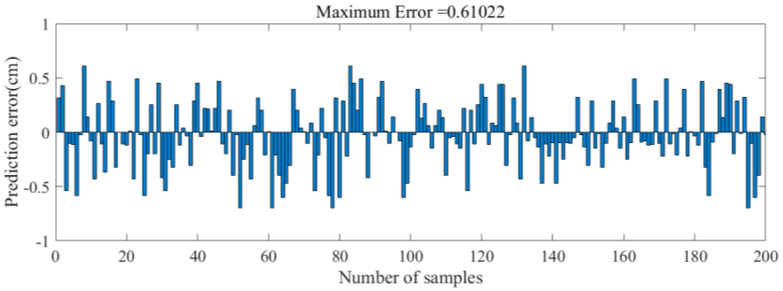
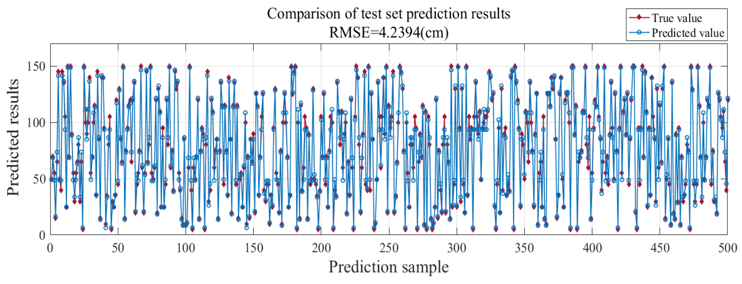
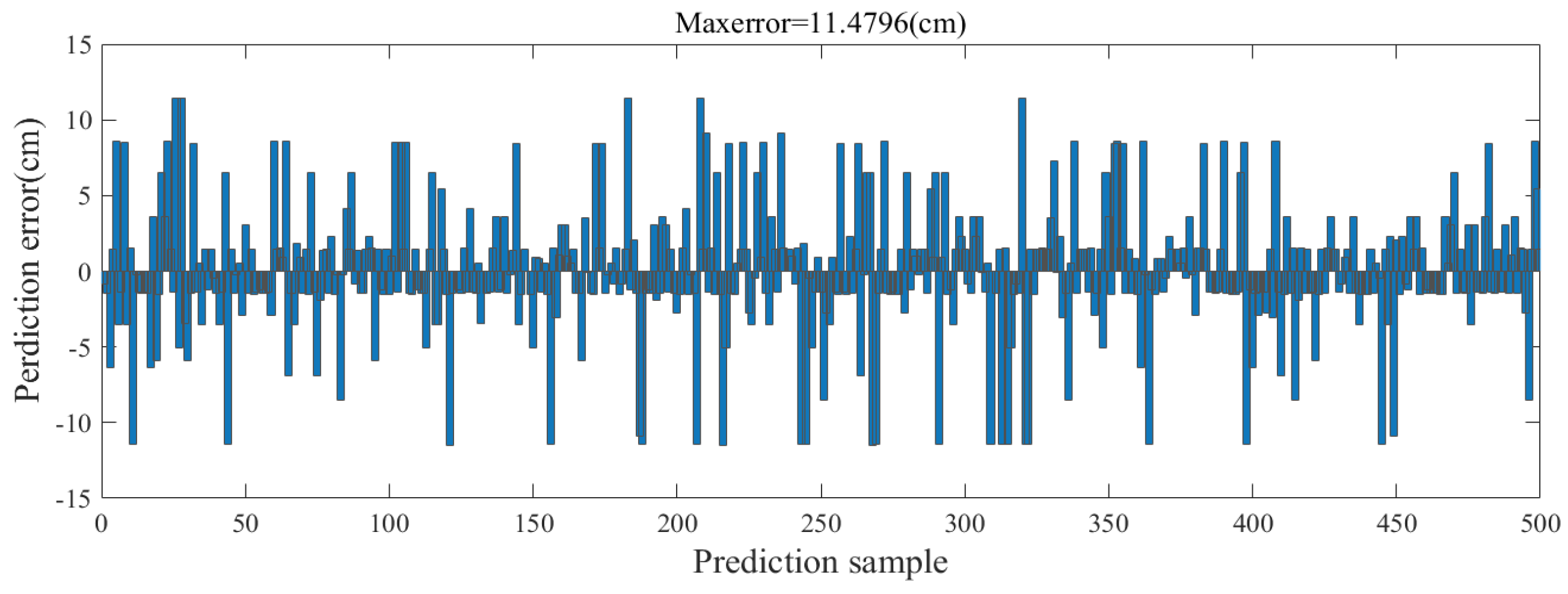
5.3. Single Tag Close–Distance Perception Model Improvement Algorithm

Two hundred different tags are randomly selected for distance perception, and the RSSI and phase feature information of the tags are collected and imported into the single tag distance perception model. Shown in Figure 29 is the comparison of single tag distance prediction without phase cycle $k$ adjustment and with phase cycle $k$ adjustment.

It is verified that the accuracy of the predicted phase period $k$ of the Single Tag Distance Perception Model without phase period $k$ adjustment is 88%, and the probability of the predicted distance error greater than $\lambda /2$ is 12%. The accuracy of the predicted phase period $k$ of the single tag distance perception model with phase period $k$ adjustment is 99%, and the accuracy of the $k$ value is significantly improved.

In summary, the system obtains more accurate distance values with an error of less than 3 cm when the distance of the tag from the RFID antenna is less than 1.5 m. The accurate distance information obtained by the system can be used for the precise positioning of RFID items, which has a wide and urgent practical need in engineering applications such as item finding, tracking, and delivery of RFID robots in mobile scenarios.

5.4. Comparison with Different Positioning Methods

This section analyzes the running time of tag group distance perception, tag group orientation perception, and single–tag position perception algorithms, and compares the tag position perception method proposed in this paper with other localization techniques.

The experiment is conducted in a scenario with a tag density of 100, and the runtime of each algorithm is measured using 1000 sets of test data, as shown in

Table 5. The running time of the algorithm.

Algorithm	Time (s)
Tag group distance perception	0.651 s
Tag group orientation perception	1.34 s
Single–Tag distance Perception	5.34 s

. From the table, tag group distance perception is shorter and more efficient, while single–tag position perception requires a combination of tag group orientation perception and single–tag distance perception algorithms, which take longer to run.

This paper compares the RFID tag positioning method proposed in this study with location techniques based on RSSI, phase–based localization, and phase difference–based localization.

Table 6. Comparison with different positioning methods.

Ref.	Localization Algorithm	Accuracy	Range	Scenario	Time Consumption
[15]	RSSI, BKNN	About 15 cm	3.8 m × 4.8 m	Static	Normal
[16]	RSSI, PSO–SVR	About 12 cm	8 m × 8 m	Simulation experiment	Low
[17]	Phase, SAR	Centimeter–level	8 m × 6 m	Dynamic	High
[18]	Phase difference	22 cm	2.4 m × 2.4 m	Static	Normal
[19]	Phase, camera	3D 25 cm	1.4 m × 1.2 m	Dynamic	Normal
[20]	Phase difference, SAR	3D 2.3 cm	2 m × 2 m	Dynamic	Normal
The proposed method	RSSI, SoI, GWO–MLP	50 cm	6 m × 6 m	Dynamic	Low
	RSSI, Phase, SVR–RANSAC	About 3 cm	1.5 m × 1.5 m	Dynamic	High

presents the comparison results, and based on Table 5 and Table 6, it can be observed that the tag group distance perception method proposed in this paper has lower positioning accuracy, but requires less time, making it suitable for applications that do not require high precision positioning. On the other hand, the single tag location perception method proposed in this paper has a longer time consumption but offers higher localization accuracy, making it suitable for applications that require precise positioning. By combining these two methods, long–distance tag localization with high precision can be achieved. In contrast, other localization methods with lower time consumption have larger localization errors, while methods with longer time consumption have smaller localization ranges. Therefore, the advantages of the tag location perception method proposed in this paper are more prominent, and it can be applied to a wide range of scenarios.

6. Conclusions

To solve the classification and finding needs of library books and logistics parcels in indoor complex environments, this paper proposes a new method for spatial location perception of tags, which consists of three parts. Firstly, a breakthrough is made by proposing the method of tag group distance perception, which goes beyond the traditional approach of precise positioning with a single tag. Before distance perception, item category numbers are added to the EPC numbers of tags attached to different packages, books, or files. Based on these category numbers, during tag group distance perception, the tag groups are automatically divided into different groups, enabling not only classification management of items but also addressing the issue of RFID robots treating all tags as a single group, which leads to significant errors in tag group distance perception. The model for RFID tag distance perception utilizes the RSSI and SoI returned by the tags as sample data to establish a distance intervals classification model for tag groups. The hyperparameters of the MLP neural network are optimized using the grey wolf optimization technique to enhance the classification accuracy. Through testing and validation, the accuracy of RFID tag group distance classification reaches 94.333%, demonstrating that the GWO–MLP classification model meets the requirements for engineering applications in mobile scenarios.

Secondly, a tag group orientation prediction algorithm is proposed, which can refine the tag group into several sub–tag groups and effectively output the specific orientations of each sub–tag group. This not only improves the accuracy of tag group positioning but also enhances the applicability and engineering value of the entire model in practical applications. The accuracy of this algorithm in orientation prediction reaches 97%, and the prediction results are quite good. Finally, to achieve precise searching for a single tag, this paper proposes a close–distance perception method for a single tag that uses the characteristic that RSSI attenuates with the increasing distance from the tag to the antenna to determine the number of cycles experienced by the phase. The method solves the problem of position ambiguity caused by phase periodicity and realizes accurate position perception based on phase. Due to the uncertainty of wavelength in the actual test, the reference distance is introduced in this paper. The k–value adjustment algorithm is proposed to improve the perception accuracy, and the prediction distance error is controlled within the range of ±3 cm. The method proposed in this paper can cater to various application requirements in different scenarios. For the need to determine the approximate position of the tag, the tag group distance perception method can be adopted. For precise tag positioning, a combination of all three methods is employed to achieve high–precision position perception.

Considering the environmental perception requirements of RFID systems in mobile scenarios, future research will focus on the following two aspects:

• The propagation model of the UHF RFID system will be deeply studied to identify the reading blind area caused by antenna polarization mismatch and multipath fading, to improve the granularity of the tag direction perception model;
• Research on phased array antennas, which enable beamforming control by manipulating the high and low levels of the antenna elements, to achieve more precise and efficient tag position perception.

References

1. Zhao, A.; Sunny, A.I.; Li, L.; Wang, T. Machine Learning-Based Structural Health Monitoring Using RFID for Harsh Environmental Conditions. Electronics 2022, 11, 1740. [Google Scholar] [CrossRef]
2. Liu, B.; Xu, H.; Zhou, X. Resource Allocation in Wireless-Powered Mobile Edge Computing Systems for Internet of Things Applications. Electronics 2019, 8, 206. [Google Scholar] [CrossRef]
3. Wu, H.; Tao, B.; Gong, Z.; Yin, Z.; Ding, H. A Standalone RFID-Based Mobile Robot Navigation Method Using Single Passive Tag. IEEE Trans. Autom. Sci. Eng. 2020, 18, 1529–1537. [Google Scholar] [CrossRef]
4. Khan, Z.; Chen, X.; He, H.; Xu, J.; Wang, T.; Cheng, L.; Ukkonen, L.; Virkki, J. Glove-Integrated Passive UHF RFID Tags—Fabrication, Testing and Applications. IEEE J. Radio Freq. Identif. 2019, 3, 127–132. [Google Scholar] [CrossRef]
5. Zhao, N.; Zhang, L.; Lei, L.; Cai, S. Dynamic Query Tree Anti-Collision Protocol for RFID Systems. In Proceedings of the 2019 IEEE 25th International Conference on Parallel and Distributed Systems (ICPADS), Tianjin, China, 4–6 December 2019. [Google Scholar]
6. Montanaro, T.; Sergi, I.; Motroni, A.; Buffi, A.; Nepa, P.; Pirozzi, M.; Catarinucci, L.; Colella, R.; Chietera, F.P.; Patrono, L. An IoT-Aware Smart System Exploiting the Electromagnetic Behavior of UHF-RFID Tags to Improve Worker Safety in Outdoor Environments. Electronics 2022, 11, 717. [Google Scholar] [CrossRef]
7. Li, C.; Mo, L.; Zhang, D. Review on UHF RFID Localization methods. IEEE J. Radio Freq. Identif. 2019, 3, 205–215. [Google Scholar] [CrossRef]
8. Dobrev, Y.; Vossiek, M.; Christmann, M.; Bilous, I.; Gulden, P. Steady Delivery: Wireless Local Positioning Systems for Tracking and Autonomous Navigation of Transport Vehicles and Mobile Robots. IEEE Microw. Mag. 2017, 18, 26–37. [Google Scholar] [CrossRef]
9. Zhou, J.; Shi, J. RFID localization algorithms and applications—A review. J. Intell. Manuf. 2009, 20, 695–707. [Google Scholar] [CrossRef]
10. Ni, L.M.; Liu, Y.; Lau, Y.C.; Patil, A.P. LANDMARC: Indoor Location Sensing Using Active RFID. In Proceedings of the First IEEE International Conference on Pervasive Computing and Communications, Fort Worth, TX, USA, 23–26 March 2003. [Google Scholar]
11. Zhao, Y.; Liu, Y.; Ni, L.M. VIRE: Active RFID-based Localization Using Virtual Reference Elimination. In Proceedings of the 2007 International Conference on Parallel Processing (ICPP 2007), Xi’an, China, 10–14 September 2007; p. 56. [Google Scholar]
12. Ma, Y.; Wang, B.; Pei, S.; Zhang, Y.; Zhang, S.; Yu, J. An Indoor Localization Method Based on AOA and PDOA Using Virtual Stations in Multipath and NLOS Environments for Passive UHF RFID. IEEE Access 2018, 6, 31772–31782. [Google Scholar] [CrossRef]
13. Ai, Z.; Liu, Y. Research on the TDOA measurement of active RFID real time location system. In Proceedings of the 2010 3rd International Conference on Computer Science and Information Technology, Chengdu, China, 9–11 July 2010; Volume 2, pp. 410–412. [Google Scholar]
14. Qi, Y.; Luo, P.; XU, C.; Wan, J.; He, J. Target Localization in Industrial Environment based on TOA Ranging. In Proceedings of the 2019 28th Wireless and Optical Communications Conference (WOCC), Beijing, China, 9–10 May 2019; pp. 1–5. [Google Scholar]
15. Xu, H.; Ding, Y.; Li, P.; Wang, R.; Li, Y. An RFID Indoor Positioning Algorithm Based on Bayesian Probability and K-Nearest Neighbor. Sensors 2017, 17, 1806. [Google Scholar] [CrossRef] [PubMed]
16. Yang, L.; Liu, Q.; Xu, J.; Hu, J.; Song, T. An indoor RFID location algorithm based on support vector regression and particle swarm optimization. In Proceedings of the 2018 IEEE 88th Vehicular Technology Conference (VTC-Fall), Chicago, IL, USA, 27–30 August 2018; pp. 1–6. [Google Scholar]
17. Bernardini, F.; Buffi, A.; Fontanelli, D.; Macii, D.; Magnago, V.; Marracci, M.; Motroni, A.; Nepa, P.; Tellini, B. Robot-Based Indoor Positioning of UHF-RFID Tags:The SAR Method with Multiple Trajectories. IEEE Trans. Instrum. Meas. 2021, 70, 1–15. [Google Scholar] [CrossRef]
18. Zeng, Y.; Chen, X.; Li, R.; Tan, H.Z. UHF RFID Indoor Positioning System with Phase Interference Model Based on Double Tag Array. IEEE Access 2019, 7, 76768–76778. [Google Scholar] [CrossRef]
19. Chatzistefanou, A.R.; Dimitriou, A.G. Tag Localization by Handheld UHF RFID Reader and Optical Markers. In Proceedings of the 2022 IEEE 12th International Conference on RFID Technology and Applications (RFID-TA), Caligari, Italy, 12–14 September 2022; pp. 9–12. [Google Scholar] [CrossRef]
20. Chu, Y.; Ma, Y.; Huang, K.; Fu, Y. A Fast Method for 3D Localization in SAR RFID System. In Proceedings of the 2022 IEEE 12th International Conference on RFID Technology and Applications (RFID-TA), Caligari, Italy, 12–14 September 2022; pp. 25–28. [Google Scholar]
21. Friis, H.T. A Note on a Simple Transmission Formula. Proc. IRE 1946, 34, 254–256. [Google Scholar] [CrossRef]
22. Mirjalili, S.; Mirjalili, S.M.; Lewis, A.D. Grey Wolf Optimizer. Adv. Eng. Softw. 2014, 69, 46–61. [Google Scholar] [CrossRef]
23. Hoppensteadt, F.C.; Izhikevich, E.M. Synaptic organizations and dynamical properties of weakly connected neural oscillators. II. Learning phase information. Biol. Cybern. 1996, 75, 117–127. [Google Scholar] [CrossRef] [PubMed]
24. Yumin, Z.; Xueshan, H.; Ming, Y.; Mingqiang, W.; Li, Z.; Pingfeng, Y.E.; Bo, X.U. Distributionally Robust Unit Commitment Based on Imprecise Dirichlet Model. In Proceedings of the CSEE 2019, Fredricton, NB, Canada, 18–21 August 2019. [Google Scholar]
25. Statnikov, A.; Hardin, D.; Guyon, I.; Aliferis, C.F. A Gentle Introduction to Support Vector Machines in Biomedicine; World Scientific Publishing Co., Pte Ltd.: Singapore, 2011. [Google Scholar]
26. Impinj. Speedway RAIN RFID Readers. 2020. Available online: https://www.impinj.com/products/readers/impinj-speedway (accessed on 7 June 2023).
27. Liu, T.; Yang, L.; Lin, Q.; Guo, Y.; Liu, Y. Anchor-free backscatter positioning for RFID tags with high accuracy. In Proceedings of the Infocom 2014, Toronto, ON, Canada, 27 April–2 May 2014. [Google Scholar]
28. Yang, L.; Chen, Y.; Li, X.Y.; Xiao, C.; Liu, Y. Tagoram: Real-time tracking of mobile RFID tags to high precision using COTS devices. In Proceedings of the 20th Annual International Conference on Mobile Computing and Networking, Maui, HI, USA, 7–11 September 2014. [Google Scholar]
29. Di Giampaolo, E.; Martinelli, F. Mobile Robot Localization Using the Phase of Passive UHF RFID Signals. IEEE Trans. Ind. Electron. 2014, 61, 365–376. [Google Scholar] [CrossRef]
30. Chum, O.; Matas, J. Optimal Randomized RANSAC. IEEE Trans. Pattern Anal. Mach. Intell. 2008, 30, 1472–1482. [Google Scholar] [CrossRef] [PubMed]
Figure 1. RFID robot indoor tag position perception flow chart.
Electronics 12 04076 g001
Figure 2. (a) The tag returns RSSI with distance. (b) The SoI and RSSI feature data in different distance intervals are non–linearly separable.
Electronics 12 04076 g002
Figure 3. The social hierarchy of the gray wolf.
Electronics 12 04076 g003
Figure 4. MLP model structure diagram.
Electronics 12 04076 g004
Figure 5. Antenna Energy Density Variation illustration.
Electronics 12 04076 g005
Figure 6. Schematic diagram of RF signal propagation process.
Electronics 12 04076 g006
Figure 7. Testing Equipment. (a) UHF RFID Indoor Inventory Robot; (b) Hardware Structure of UHF RFID Inventory Robot.
Electronics 12 04076 g007
Figure 8. Software Architecture of RFID Robot Indoor Inventory System.
Electronics 12 04076 g008
Figure 9. Test Environment. (a) Indoor tag position perception test scenario. (b) Experimental map of position perception of UHF passive RFID tags.
Electronics 12 04076 g009
Figure 10. Archive Management Application Scenarios.
Electronics 12 04076 g010
Figure 11. Tag group distance perception flow chart.
Electronics 12 04076 g011
Figure 12. GWO optimization algorithm adaptation curve.
Electronics 12 04076 g012
Figure 13. RFID tag group distance interval classification results.
Electronics 12 04076 g013
Figure 14. Tag Group Orientation Perception Illustration. (a) Coordinate system for the rotation angle of the reader antenna. (b) Figure depicting the division of three tag groups. (c) Figure depicting the division of nine tag groups.
Electronics 12 04076 g014
Figure 15. Single tag distance perception flow chart.
Electronics 12 04076 g015
Figure 16. Relationship between RSSI and distance.
Electronics 12 04076 g016
Figure 17. Relationship between phase and distance variation.
Electronics 12 04076 g017
Figure 18. Schematic diagram of RSSI estimated phase period.
Electronics 12 04076 g018
Figure 19. RANSAC linear regression model of phase versus distance.
Electronics 12 04076 g019
Figure 20. Phase prediction distance error diagram.
Electronics 12 04076 g020
Figure 21. SVR prediction results graph.
Electronics 12 04076 g021
Figure 22. Prediction distance error graph.
Electronics 12 04076 g022
Figure 23. Regression curve of RSSI and tag distance.
Electronics 12 04076 g023
Figure 24. RFID tag group distance prediction results.
Electronics 12 04076 g024
Figure 25. Confusion matrix of GWO–MLP classification model.
Electronics 12 04076 g025
Figure 26. Antenna Angle Calculation illustration.
Electronics 12 04076 g026
Figure 27. Distribution of Tag Group Positions.
Electronics 12 04076 g027
Figure 28. Tag group subdivision and orientation prediction result.
Electronics 12 04076 g028
Figure 29. Comparison diagram of prediction results for single tag distance perception algorithm.
Electronics 12 04076 g029