
DFFA-Net: A Differential Convolutional Neural Network for Underwater Optical Image Dehazing

Abstract
:1. Introduction
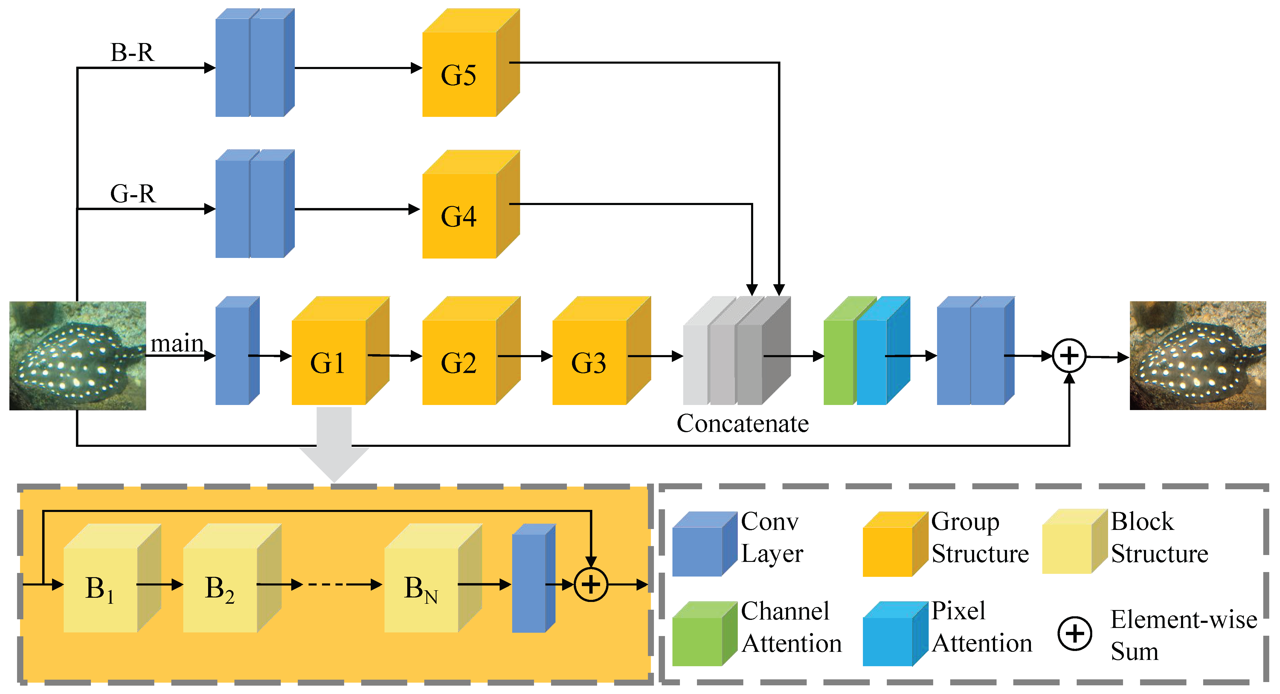
- We propose a novel underwater image dehazing model, DFFA-Net, which utilizes color channel mutual information. Building on the FFA-Net architecture, we introduce the proposed color differential modules to facilitate learning of the domain mapping between hazy images and clear images.
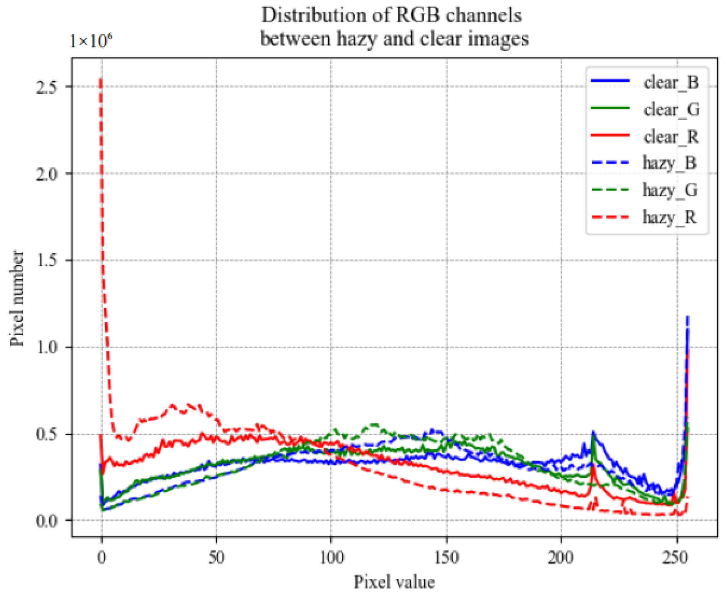
- We introduce a color channel-sensitive loss function that guides the neural network to better align the color statistical distribution of hazy images with that of clear images.
- Compared to other convolutional neural network-based dehazing models, our proposed model demonstrates superior performance in terms of evaluation metrics. Additionally, we have made the code publicly available.
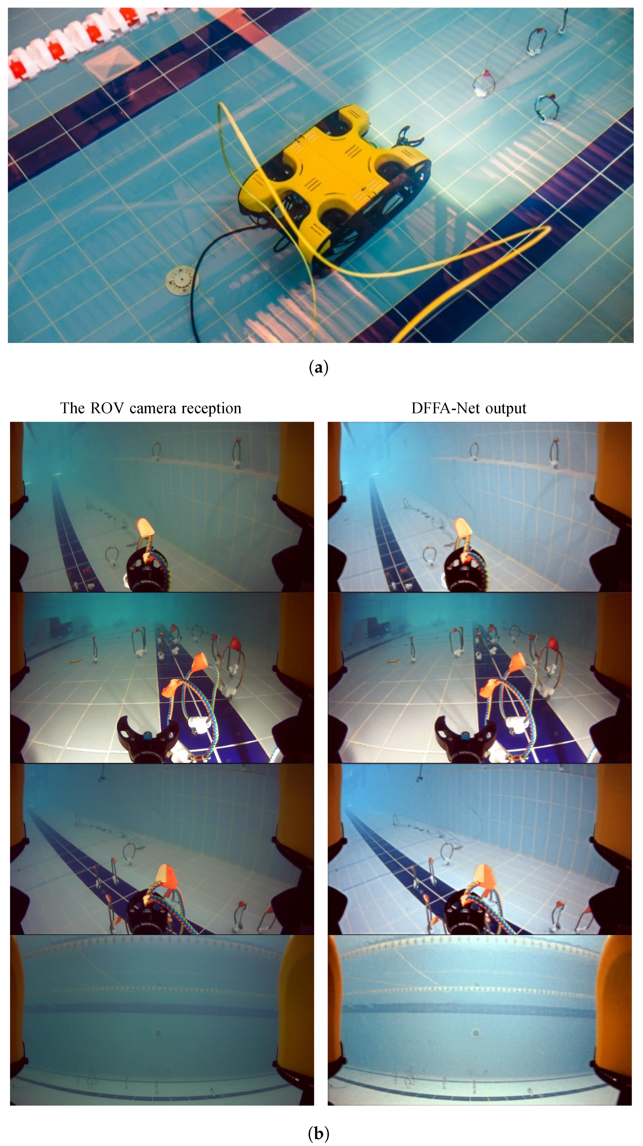
- We have successfully deployed the DFFA-Net on an ROV, allowing us to effectively obtain dehazed images. In a swimming pool environment, DFFA-Net provides real-time output images that ensure good camera image quality.
2. Related Work
3. Method
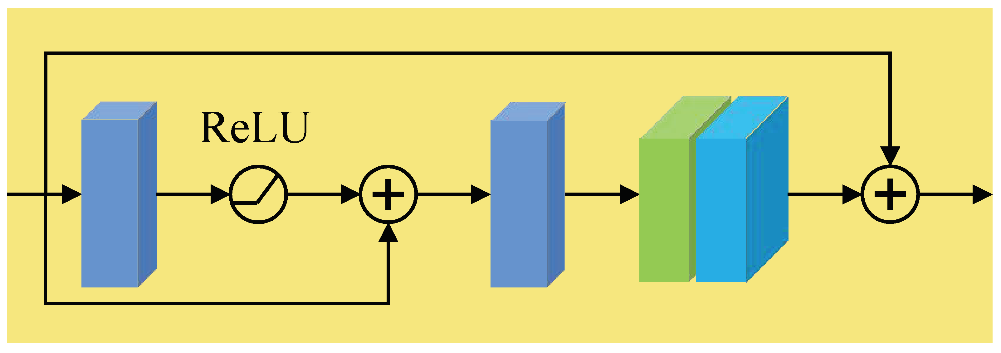
3.1. Feature Attention (FA)
- 1
- A global adaptive average pooling layer is applied to obtain a output.
- 2
- Two convolutional layers are used to downsample the number of channels from C to and then upsample it back to C. The downsampled output is then further passed through a ReLU activation function and the upsampled output is passed through a sigmoid activation function.
- 3
- The original input is multiplied element-wise by the output from Step 2.
- 1
- Two convolutional layers are used to downsample the number of channels to and 1, respectively. The output of the first convolutional layer is passed through a ReLU activation function and the output of the second convolutional layer is passed through a sigmoid activation function.
- 2
- The original input is multiplied element-wise by the output from Step 1.
3.2. Group Structure
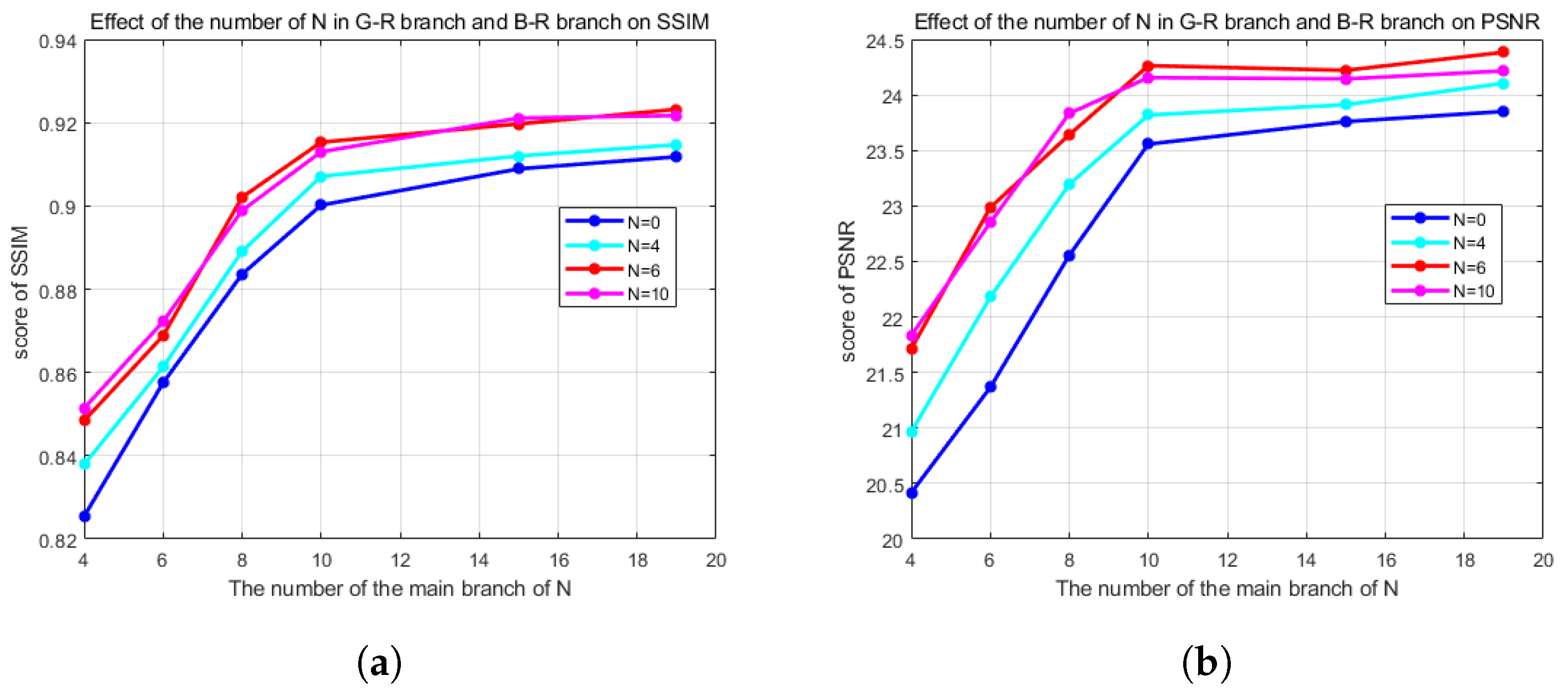
3.3. B–R and G–R
3.4. Loss
4. Experiment and Analysis
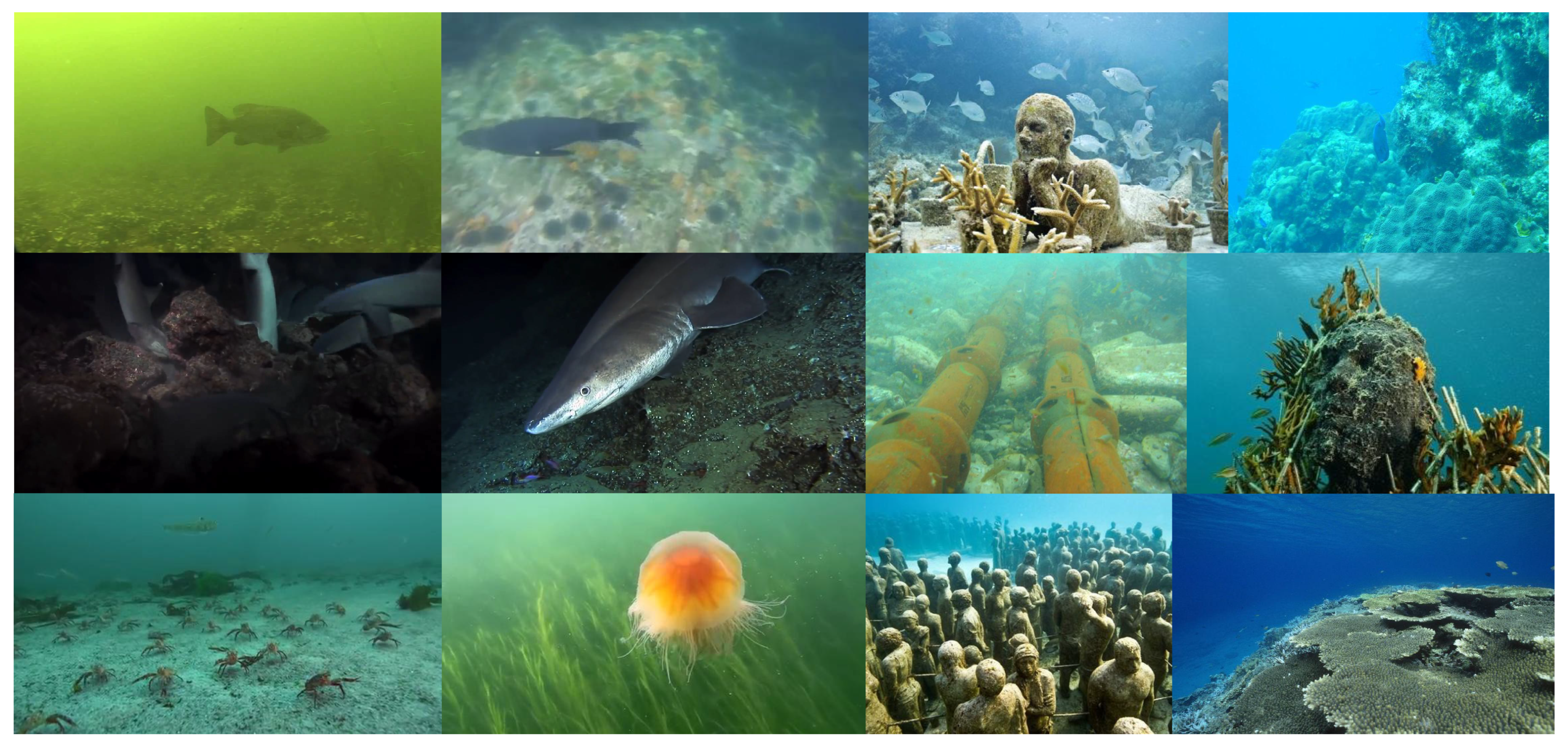
4.1. Dataset
4.2. Training
4.3. Evaluation Index of the Model
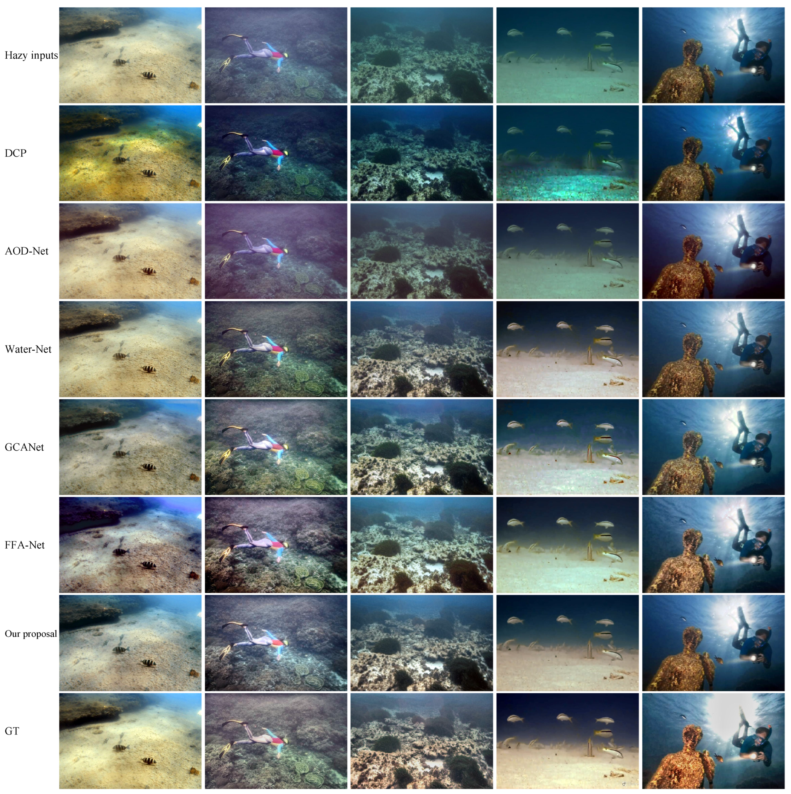
4.4. Results
5. Application
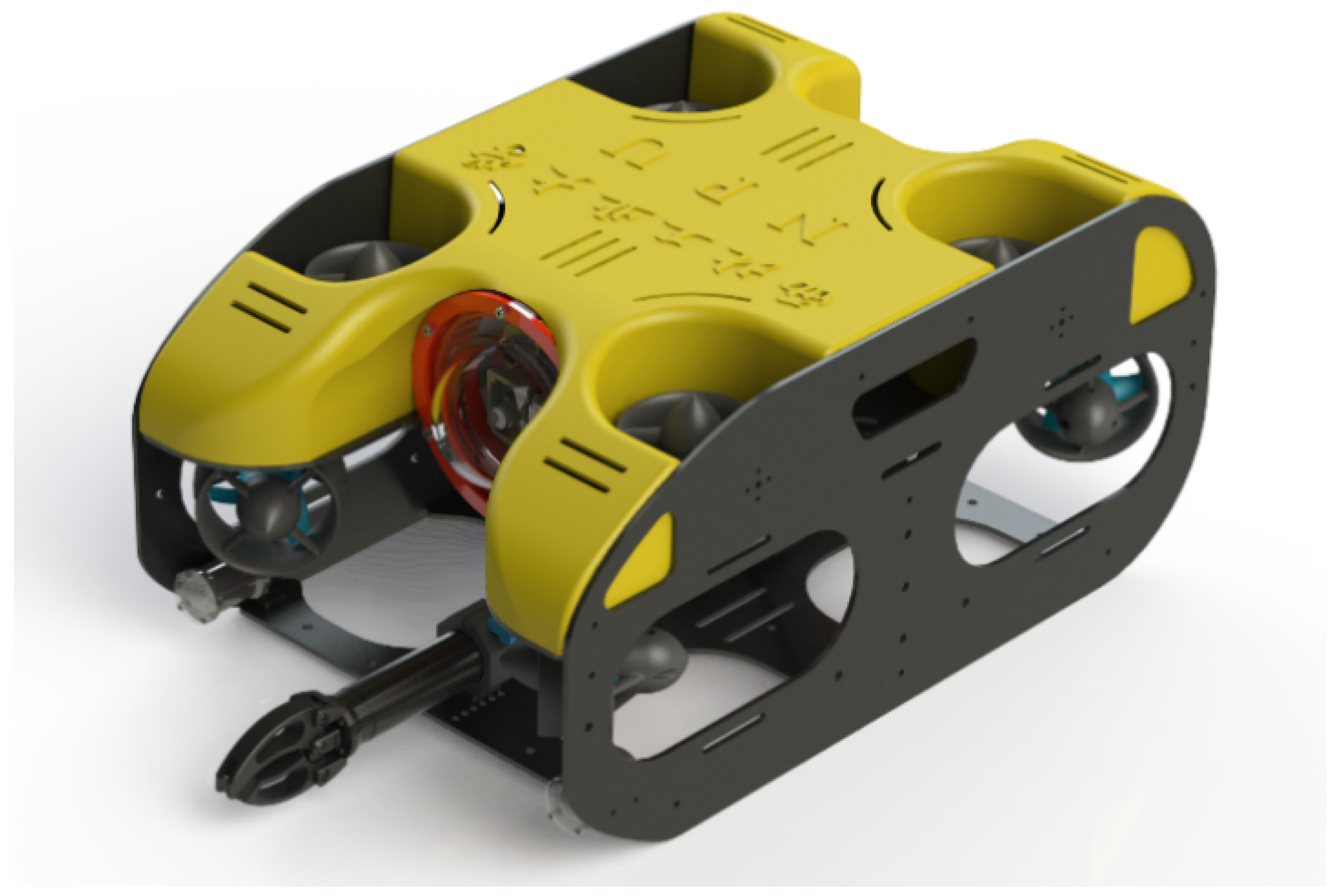
5.1. ROV Design
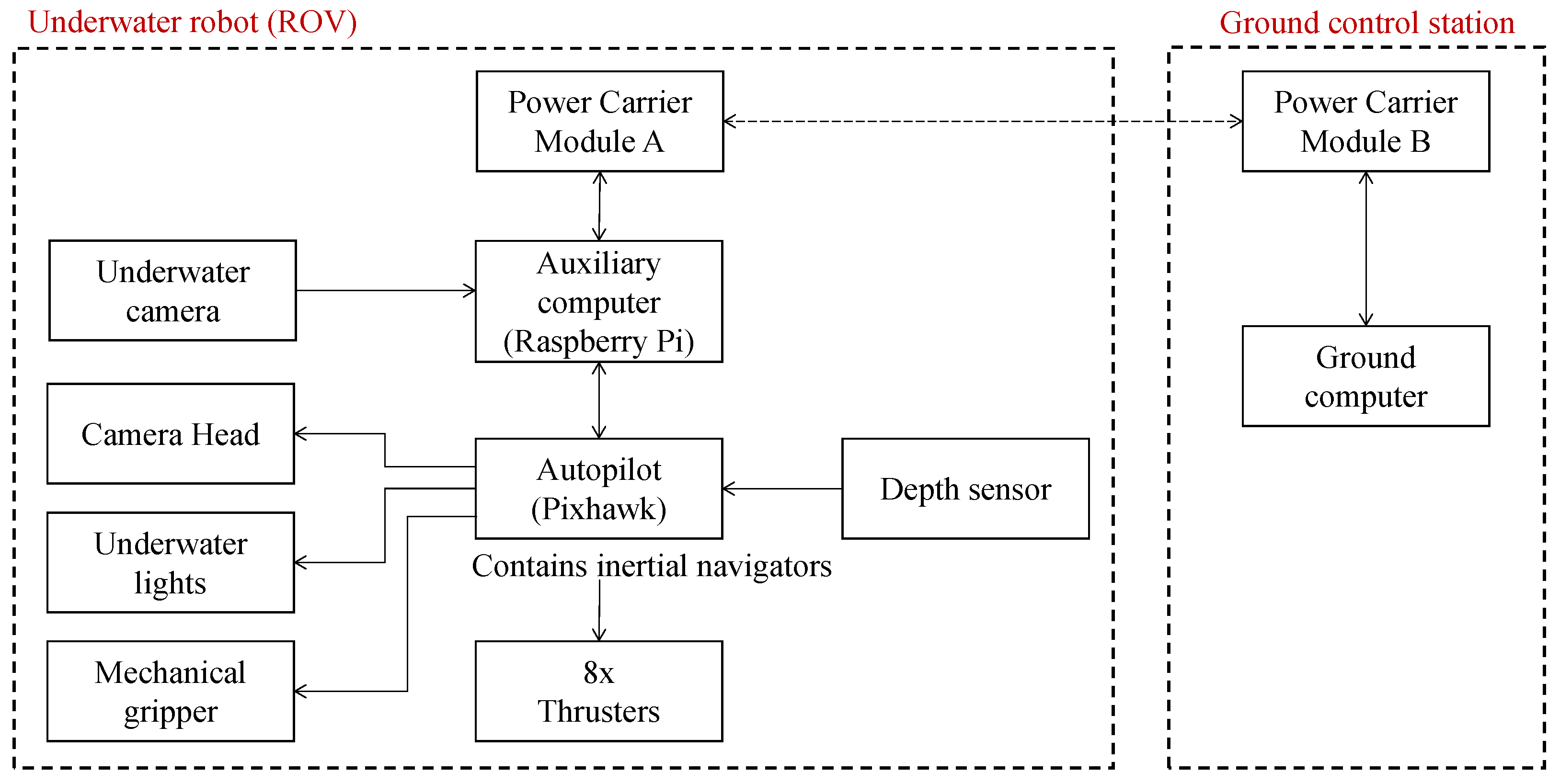
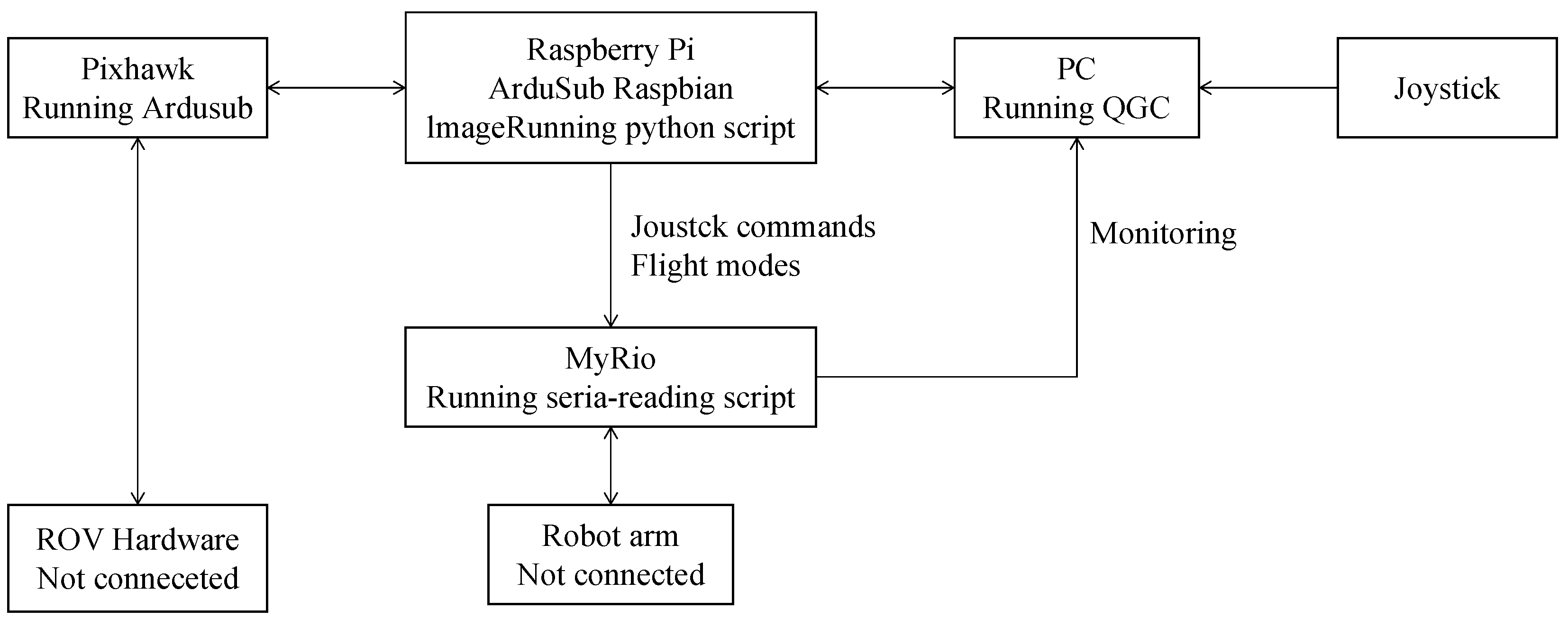
5.2. Control System Design
5.3. Real-Time Underwater Image Dehazing
6. Conclusions
Author Contributions
Funding
Data Availability Statement
Acknowledgments
Conflicts of Interest
References
- Liu, Y.; Anderlini, E.; Wang, S.; Ma, S.; Ding, Z. Ocean explorations using autonomy: Technologies, strategies and applications. In Proceedings of the Offshore Robotics, Xi’an, China, 30 May–5 June 2021; Springer: Berlin/Heidelberg, Germany, 2022; pp. 35–58. [Google Scholar]
- Egg, L.; Pander, J.; Mueller, M.; Geist, J. Comparison of sonar-, camera-and net-based methods in detecting riverine fish-movement patterns. Mar. Freshw. Res. 2018, 69, 1905–1912. [Google Scholar] [CrossRef]
- Terayama, K.; Shin, K.; Mizuno, K.; Tsuda, K. Integration of sonar and optical camera images using deep neural network for fish monitoring. Aquac. Eng. 2019, 86, 102000. [Google Scholar] [CrossRef]
- Schettini, R.; Corchs, S. Underwater image processing: State of the art of restoration and image enhancement methods. Eurasip J. Adv. Signal Process. 2010, 2010, 1–14. [Google Scholar] [CrossRef]
- Sahu, P.; Gupta, N.; Sharma, N. A survey on underwater image enhancement techniques. Int. J. Comput. Appl. 2014, 87, 333–338. [Google Scholar] [CrossRef]
- Zhang, W.; Zhuang, P.; Sun, H.H.; Li, G.; Kwong, S.; Li, C. Underwater image enhancement via minimal color loss and locally adaptive contrast enhancement. IEEE Trans. Image Process. 2022, 31, 3997–4010. [Google Scholar] [CrossRef] [PubMed]
- Narasimhan, S.G.; Nayar, S.K. Chromatic framework for vision in bad weather. In Proceedings of the IEEE Conference on Computer Vision and Pattern Recognition, CVPR 2000 (Cat. No. PR00662), Hilton Head Island, SC, USA, 15 June 2000; IEEE: New York, NY, USA, 2000; Volume 1, pp. 598–605. [Google Scholar]
- Narasimhan, S.G.; Nayar, S.K. Vision and the atmosphere. Int. J. Comput. Vis. 2002, 48, 233. [Google Scholar] [CrossRef]
- He, K.; Sun, J.; Tang, X. Single image haze removal using dark channel prior. IEEE Trans. Pattern Anal. Mach. Intell. 2010, 33, 2341–2353. [Google Scholar]
- Li, B.; Peng, X.; Wang, Z.; Xu, J.; Feng, D. Aod-net: All-in-one dehazing network. In Proceedings of the IEEE International Conference on Computer Vision, Vancouver, BC, Canada, 7–14 July 2017; pp. 4770–4778. [Google Scholar]
- Chen, D.; He, M.; Fan, Q.; Liao, J.; Zhang, L.; Hou, D.; Yuan, L.; Hua, G. Gated context aggregation network for image dehazing and deraining. In Proceedings of the 2019 IEEE Winter Conference on Applications of Computer Vision (WACV), Waikoloa Village, HI, USA, 7–11 January 2019; IEEE: New York, NY, USA, 2019; pp. 1375–1383. [Google Scholar]
- Qin, X.; Wang, Z.; Bai, Y.; Xie, X.; Jia, H. FFA-Net: Feature fusion attention network for single image dehazing. In Proceedings of the AAAI Conference on Artificial Intelligence, New York, NY, USA, 7–12 February 2020; Volume 34, pp. 11908–11915. [Google Scholar]
- Fattal, R. Single image dehazing. Acm Trans. Graph. Tog 2008, 27, 1–9. [Google Scholar] [CrossRef]
- Zhu, Q.; Mai, J.; Shao, L. A fast single image haze removal algorithm using color attenuation prior. IEEE Trans. Image Process. 2015, 24, 3522–3533. [Google Scholar]
- Berman, D.; Avidan, S. Non-local image dehazing. In Proceedings of the IEEE Conference on Computer Vision and Pattern Recognition, Las Vegas, NV, USA, 26 June–1 July 2016; pp. 1674–1682. [Google Scholar]
- Meng, G.; Wang, Y.; Duan, J.; Xiang, S.; Pan, C. Efficient image dehazing with boundary constraint and contextual regularization. In Proceedings of the IEEE International Conference on Computer Vision, Washington, DC, USA, 1–8 December 2013; pp. 617–624. [Google Scholar]
- Shin, J.; Kim, M.; Paik, J.; Lee, S. Radiance–reflectance combined optimization and structure-guided ℓ0-Norm for single image dehazing. IEEE Trans. Multimed. 2019, 22, 30–44. [Google Scholar] [CrossRef]
- Cai, B.; Xu, X.; Jia, K.; Qing, C.; Tao, D. Dehazenet: An end-to-end system for single image haze removal. IEEE Trans. Image Process. 2016, 25, 5187–5198. [Google Scholar] [CrossRef] [PubMed]
- Li, C.; Guo, C.; Ren, W.; Cong, R.; Hou, J.; Kwong, S.; Tao, D. An Underwater Image Enhancement Benchmark Dataset and Beyond. IEEE Trans. Image Process. 2020, 29, 4376–4389. [Google Scholar] [CrossRef] [PubMed]
- Ren, W.; Liu, S.; Zhang, H.; Pan, J.; Cao, X.; Yang, M.H. Single image dehazing via multi-scale convolutional neural networks. In Proceedings of the Computer Vision–ECCV 2016: 14th European Conference, Amsterdam, The Netherlands, 11–14 October 2016; Part II 14. Springer: Berlin/Heidelberg, Germany, 2016; pp. 154–169. [Google Scholar]
- Li, J.; Skinner, K.A.; Eustice, R.M.; Johnson-Roberson, M. WaterGAN: Unsupervised generative network to enable real-time color correction of monocular underwater images. IEEE Robot. Autom. Lett. 2017, 3, 387–394. [Google Scholar] [CrossRef]
- Zhang, R.; Isola, P.; Efros, A.A.; Shechtman, E.; Wang, O. The Unreasonable Effectiveness of Deep Features as a Perceptual Metric. In Proceedings of the IEEE Conference on Computer Vision and Pattern Recognition (CVPR), Salt Lake City, UT, USA, 18–23 June 2018. [Google Scholar]
- Simonyan, K.; Zisserman, A. Very Deep Convolutional Networks for Large-Scale Image Recognition. arXiv 2014, arXiv:1409.1556. [Google Scholar]
- Ancuti, C.; Ancuti, C.O.; Haber, T.; Bekaert, P. Enhancing underwater images and videos by fusion. In Proceedings of the 2012 IEEE Conference on Computer Vision and Pattern Recognition, Providence, RI, USA, 16–21 June 2012; IEEE: New York, NY, USA, 2012; pp. 81–88. [Google Scholar]
- Fu, X.; Fan, Z.; Ling, M.; Huang, Y.; Ding, X. Two-step approach for single underwater image enhancement. In Proceedings of the 2017 International Symposium on Intelligent Signal Processing and Communication Systems (ISPACS), Xiamen, China, 6–9 November 2017; IEEE: New York, NY, USA, 2017; pp. 789–794. [Google Scholar]
- Fu, X.; Zhuang, P.; Huang, Y.; Liao, Y.; Zhang, X.P.; Ding, X. A retinex-based enhancing approach for single underwater image. In Proceedings of the 2014 IEEE International Conference on Image Processing (ICIP), Paris, France, 27–30 October 2014; IEEE: New York, NY, USA, 2014; pp. 4572–4576. [Google Scholar]
- Drews, P.L.; Nascimento, E.R.; Botelho, S.S.; Campos, M.F.M. Underwater depth estimation and image restoration based on single images. IEEE Comput. Graph. Appl. 2016, 36, 24–35. [Google Scholar] [CrossRef]
- Li, C.; Guo, J.; Guo, C.; Cong, R.; Gong, J. A hybrid method for underwater image correction. Pattern Recognit. Lett. 2017, 94, 62–67. [Google Scholar] [CrossRef]
- Peng, Y.T.; Cao, K.; Cosman, P.C. Generalization of the dark channel prior for single image restoration. IEEE Trans. Image Process. 2018, 27, 2856–2868. [Google Scholar] [CrossRef]
- Galdran, A.; Pardo, D.; Picón, A.; Alvarez-Gila, A. Automatic red-channel underwater image restoration. J. Vis. Commun. Image Represent. 2015, 26, 132–145. [Google Scholar] [CrossRef]
- Li, C.Y.; Guo, J.C.; Cong, R.M.; Pang, Y.W.; Wang, B. Underwater image enhancement by dehazing with minimum information loss and histogram distribution prior. IEEE Trans. Image Process. 2016, 25, 5664–5677. [Google Scholar] [CrossRef]
- Peng, Y.T.; Cosman, P.C. Underwater image restoration based on image blurriness and light absorption. IEEE Trans. Image Process. 2017, 26, 1579–1594. [Google Scholar] [CrossRef]
- Ancuti, C.O.; Ancuti, C.; De Vleeschouwer, C.; Bekaert, P. Color balance and fusion for underwater image enhancement. IEEE Trans. Image Process. 2017, 27, 379–393. [Google Scholar] [CrossRef] [PubMed]
- Wang, Z.; Bovik, A.C.; Sheikh, H.R.; Simoncelli, E.P. Image quality assessment: From error visibility to structural similarity. IEEE Trans. Image Process. 2004, 13, 600–612. [Google Scholar] [CrossRef] [PubMed]


| Method | SSIM ↑ | PSNR ↑ | Model Size (MB) | Inference Time (ms) |
|---|---|---|---|---|
| DCP | 0.7468 | 15.2346 | - | 166.43 |
| AODNet | 0.8244 | 19.2519 | 0.14 | 29.13 |
| WaterNet | 0.9115 | 23.4502 | 4.17 | 68.86 |
| GCANet | 0.9025 | 23.1840 | 4.42 | 76.97 |
| FFANet | 0.9118 | 23.5567 | 17.74 | 110.81 |
| Our proposal | 0.9153 | 24.2631 | 13.20 | 90.21 |
| Maneuvering ability | Forward, backward, transverse, snorkeling, pitch, roll, yaw |
| Moving speed | Stepless speed regulation |
| Whether to support multiple maneuvering operations at the same time | Support |
| Attitude control | Pitch Angle holding function (±20°) Roll Angle holding function (±20°) |
| Input hold function | One key lock the current control execution command, so that the robot maintains the current speed, depth, heading Angle and attitude of continuous navigation |
| Control mode | Manual mode, stable mode, fixed depth mode |
| Video recording capability | Support |
| Hand bite force | 10 Kg |
| Design depth | 50 m |
| Endurance time | 2 to 3 h |
Disclaimer/Publisher’s Note: The statements, opinions and data contained in all publications are solely those of the individual author(s) and contributor(s) and not of MDPI and/or the editor(s). MDPI and/or the editor(s) disclaim responsibility for any injury to people or property resulting from any ideas, methods, instructions or products referred to in the content. |
© 2023 by the authors. Licensee MDPI, Basel, Switzerland. This article is an open access article distributed under the terms and conditions of the Creative Commons Attribution (CC BY) license (https://creativecommons.org/licenses/by/4.0/).
Share and Cite
Hou, X.; Zhang, F.; Wang, Z.; Song, G.; Huang, Z.; Wang, J. DFFA-Net: A Differential Convolutional Neural Network for Underwater Optical Image Dehazing. Electronics 2023, 12, 3876. https://doi.org/10.3390/electronics12183876
Hou X, Zhang F, Wang Z, Song G, Huang Z, Wang J. DFFA-Net: A Differential Convolutional Neural Network for Underwater Optical Image Dehazing. Electronics. 2023; 12(18):3876. https://doi.org/10.3390/electronics12183876
Chicago/Turabian StyleHou, Xujia, Feihu Zhang, Zewen Wang, Guanglei Song, Zijun Huang, and Jinpeng Wang. 2023. "DFFA-Net: A Differential Convolutional Neural Network for Underwater Optical Image Dehazing" Electronics 12, no. 18: 3876. https://doi.org/10.3390/electronics12183876