Article

High-Level K-Nearest Neighbors (HLKNN): A Supervised Machine Learning Model for Classification Analysis

1
Independent Researcher, Izmir 35390, Turkey
2
Graduate School of Natural and Applied Sciences, Dokuz Eylul University, Izmir 35390, Turkey
3
Department of Computer Engineering, Dokuz Eylul University, Izmir 35390, Turkey
*
Author to whom correspondence should be addressed.
Electronics 2023, 12(18), 3828; https://doi.org/10.3390/electronics12183828
Submission received: 14 August 2023 / Revised: 6 September 2023 / Accepted: 7 September 2023 / Published: 10 September 2023
(This article belongs to the Special Issue Advances in Data Science: Methods, Systems, and Applications)

Abstract

:
The k-nearest neighbors (KNN) algorithm has been widely used for classification analysis in machine learning. However, it suffers from noise samples that reduce its classification ability and therefore prediction accuracy. This article introduces the high-level k-nearest neighbors (HLKNN) method, a new technique for enhancing the k-nearest neighbors algorithm, which can effectively address the noise problem and contribute to improving the classification performance of KNN. Instead of only considering k neighbors of a given query instance, it also takes into account the neighbors of these neighbors. Experiments were conducted on 32 well-known popular datasets. The results showed that the proposed HLKNN method outperformed the standard KNN method with average accuracy values of 81.01% and 79.76%, respectively. In addition, the experiments demonstrated the superiority of HLKNN over previous KNN variants in terms of the accuracy metric in various datasets.

1. Introduction

Machine learning (ML) is a technique to equip a system with the capability of predicting future events. It utilizes various algorithms to analyze historical data and learn from them with the intention of forecasting new outcomes for unseen data. Actually, it attempts to discover patterns in past experiences hidden in related data through the training process and generates a predictive model. Nowadays, machine learning plays notable roles in different fields to contribute to making effective decisions in organizations. It is worth emphasizing that ML is currently an essential concept to extend the artificial intelligence (AI) of smart systems by alleviating human interventions because of their limited brain and memory capacities. AI is a research area in computer science that aims to simulate human-like thoughts in machines applicable in many fields, including industry, health, security, transportation, energy, and commerce. Also, artificial intelligence paves the route for the advent of modern technologies struggling to automate tasks and act independently from individuals [1].
There is a wide range of applications of ML, such as anomaly detection to identify abnormal items, recommendation systems to offer items to users, clustering to group similar items, regression for predicting numerical values, and classification to categorize items. Bearing this in mind, ML applications rely on the extraction of patterns and regularities from the previous related data. Therefore, the reproducibility and reusability of ML-based models make them appropriate in many fields such as intelligent decision-making, fraud detection, image processing, financial analytics, facial recognition, Internet of Things (IoT), natural language processing, and user behavior analytics [2].
Based on the type of problems to be solved by ML concepts, there are various categories for learning, including reinforcement, unsupervised, supervised, and semisupervised learning. In reinforcement learning, the ML model relies on rewards during agent–environment interactions. Its purpose is to assess optimal behaviors that enhance the environment. It is widely used in the domains of robotics, gaming, advertising, and manufacturing. In unsupervised learning, the ML model attempts to learn from an unlabeled dataset, for instance, in anomaly detection, density estimation, and clustering tasks. The other type of machine learning algorithm is supervised learning, which only learns from labeled data to find out a suitable mapping function. It is commonly used in credit scoring, sentiment analysis, email filtering, and risk assessment [3]. Semisupervised learning is a combination of unsupervised and supervised learning techniques utilizing both unlabeled and labeled data in its learning process, including applications such as fraud detection, speech analysis, and text classification.
Classification is a type of supervised learning technique, which is extensively used to generate various ML models with the purpose of class label prediction in a related dataset. There are many classification methods proposed in machine learning literature for a broad range of applications. The following are the most well-known classification algorithms: naive Bayes, random forest, decision trees, support vector machines, and neural networks. Moreover, the k-nearest neighbors (KNN) algorithm is one of the most significant classification algorithms, which can be applied to regression tasks, too. KNN is an instance-based learning methodology, also called “lazy learning”. It means that the training dataset is postponed to be completely processed until encountering a given test query for prediction via this algorithm. Actually, KNN can perform an exhaustive search in large dimensions. In the KNN classifier, the training set is supposed as an m-dimensional space of patterns for searching the k-closest tuples to a given test query. The closeness is described in terms of a specific distance metric, e.g., Euclidean distance. Additionally, the min–max normalization approach is applicable to balance the effect of various ranges before calculating the distance [4].
In this study, we improved the KNN algorithm due to its advantages such as effectiveness, easy implementation, and simplicity [5]. The benefits of KNN also include ease of interpretation and understanding of the results. Furthermore, it has the ability to predict both discrete and categorical variables; thus, it can be utilized for both regression and classification tasks. Another advantage of KNN is the independence of any data distribution since it uses local neighborhoods. Moreover, it can easily support incremental data since the training process is not needed for the newly arrived samples. The standard KNN algorithm has been proven to be an effective method in many studies [6].
Even though KNN is effective in many cases, it has a shortcoming that reduces its classification ability. Noisy data samples are a considerable limitation since they only search the nearest neighbors of a test instance, and these samples affect the result of the neighborhood concept, so all of these affect the accuracy. The proposed method in this paper decreases this limitation by enhancing the search process.
The main contributions and novel aspects of this study are summarized as follows:
  • This paper proposes a machine learning method, named high-level k-nearest neighbors (HLKNN), based on the KNN algorithm.
  • It contributes to improving the KNN approach since the noisy samples inefficiently affect its classification ability.
  • Our work is original in that the HLKNN model was applied to 32 benchmark datasets to predict the related target values with the objective of model evaluation.
  • The experimental results revealed that HLKNN outperformed KNN on 26 out of 32 datasets in terms of classification accuracy.
  • The presented method in this study was also compared with the previous KNN variants, including uniform kNN, weighted kNN, kNNGNN, k-MMS, k-MRS, k-NCN, NN, k-NFL, k-NNL, k-CNN, and k-TNN, and the superiority of HLKNN over its counterparts was approved on the same datasets.
The rest of this paper is organized as follows. The related works are discussed in Section 2. The proposed HLKNN method is explained in detail in Section 3. The experimental studies are presented in Section 4. Eventually, the conclusion and future works of the current study are described in Section 5.

2. Related Works

First, this section briefly explains the most relevant works to our study. After that, it describes the various types of KNN algorithms in the literature.

2.1. A Review of Related Literature

K-nearest neighbors (KNN) is a supervised machine learning method that can be utilized for both classification and regression tasks. KNN considers the similarity factor between new and available data to classify an object into predefined categories. KNN has been widely used in many fields such as industry [7,8,9], machine engineering [10], health [11,12,13], marketing [14], electrical engineering [15], security [16,17,18], manufacturing [19], energy [20,21,22], aerial [23], environment [24], geology [25,26], maritime [27,28], geographical information systems (GIS) [29], and transportation [30].
In the field of industry, the authors introduced a hybrid bag of features (HBoF) in [7] to classify the multiclass health conditions of spherical tanks. In their HBoF-based approach, they extracted vital features using the Boruta algorithm. These features were then fed into the multiclass KNN to distinguish normal and faulty conditions. This KNN-based method yielded high accuracy, surpassing other advanced techniques. In [8], the authors have reported that the KNN algorithm attained a great performance according to different evaluation metrics for predicting the compressive strength of concrete. Their model was highly recommended in the construction industry owing to the fact that it required fewer computational resources to be implemented. In another work [9], a KNN-based method was developed to efficiently detect faults by considering outliers on the basis of the elbow rule for industrial processes. Similarly, in machine engineering, the authors presented a KNN-based fault diagnosis approach for rotating machinery, which was validated through testing on the bearing datasets [10].
In the field of health, Salem et al. [11] investigated a KNN-based method for diabetes classification and prediction that can contribute to the early treatment of diabetes as one of the main chronic diseases. The outperformance of their method was evaluated in terms of various metrics and approved its applicability in the healthcare system for diabetes compared to other techniques. In another work [12], the researchers focused on an approach to early detect placental microcalcification by the KNN algorithm, which could lead to the improvement of maternal and fetal health monitoring during pregnancy. The results gained from real clinical datasets revealed the efficiency of the proposed model for pregnant women. In [13], a wearable device was introduced on the basis of embedded insole sensors and the KNN machine learning model for gait analysis from the perspective of controlling prostheses. The results of applying the KNN algorithm showed the success of the device in predicting various gait phases with high accuracy.
In marketing, Nguyen et al. [14] represented a beneficial recommendation system via KNN-based collaborative filtering, in which similar users according to their cognition parameters were effectively grouped to obtain more relevant recommendations in different e-commerce activities. In the field of electrical engineering, Corso et al. [15] developed a classification approach for the insulator contamination levels by the KNN algorithm with high accuracy to predict insulating features as predictive maintenance of power distribution networks. In the field of security, a KNN-based technique was proposed in [16] to classify botnet attacks in an IoT network. In addition, the forward feature selection was utilized in their technique to obtain improved accuracy and execution time in comparison to other benchmark methods. In [17], a novel security architecture was provided to effectively deal with forged and misrouted commands in an industrial IoT considering different technologies, namely, KNN, random substance learning (RSL), software-defined network (SDN), and a blockchain-based integrity checking system (BICS). In another work [18], an intrusion detection system (IDS) was implemented for wireless sensor networks by employing KNN and arithmetic optimization algorithms in that an edge intelligence framework was utilized for denial-of-service attacks in WSNs.
In the field of manufacturing [19], Zheng et al. introduced a consensus model on the basis of KNN to classify cloud transactions regarding their priorities. In their model, different parameters, e.g., service level agreements (SLA), cloud service providers (CSP), cloud service consumers (CSC), and smart contract (SC) types, were utilized for distance calculation in the KNN algorithm. In the field of electrical energy [20], a short-term load forecasting technique was proposed by the weighted KNN algorithm to achieve high accuracy for fitting the model. Similarly, in another work [21], the authors focused on an effective KNN-based model for the failure diagnosis of wind power systems regarding particle swarm optimization. In [22], the researchers investigated seismic energy dissipation for rocking foundations in the seismic loading process by means of different supervised machine learning algorithms, including KNN, support vector regression (SVR), and decision tree regression (DTR). The k-fold cross-validation was applied to the mentioned algorithms and, according to the results, KNN and SVR outperformed DTR in terms of accuracy.
In the aerial field, Martínez-Clark et al. [23] represented a KNN-based method as a flock inspiration from nature for a group of unmanned aerial vehicles (UAVs). In their method, an optimal number of UAVs was obtained with regard to heading synchronization in drone implementation. In the environment field, a predictive model was developed in [24] for the construction and demolition waste rate forecast by means of KNN and principal component analysis (PCA). In the field of geology, the authors [25] reported that the KNN algorithm was utilized for a three-dimensional envision of the stratigraphic structure of porous media related to sedimentary formations. In a similar work in geology, Bullejos et al. [26] implemented a technique for the evaluation of KNN prediction confidence in that the three-dimensional model for the stratigraphic structure of porous media is approved. The results of their KNN-based method contributed to improving the predictability of groundwater investigations.
In the maritime field, the authors [27] introduced a novel trajectory model for offshore waters with the means of KNN and long short-term memory (LSTM) techniques for high-density and low-density trajectories, respectively. Their experimental results revealed that the mean square error is significantly decreased in comparison with the previous artificial-neural-network-based models. Another research [28] in this area employed a KNN-based approach. The authors utilized the PCA method for predictive ship maintenance, with a specific emphasis on propulsion engines. In the field of GIS, the authors [29] presented a predictive model with an ensemble KNN for typhoon tracks, which included supervised classification and regression applied on various samples of typhoons gaining experimental results with high accuracies and low running times. In the field of transportation [30], the effect of missed data was detected through the KNN classifier for the prediction of traffic flow on public roads. Their results show that the presented method was efficiently applicable for smart transportation in urban traffic control.

2.2. A Review of KNN Variants

In the literature, researchers have provided various types of KNN algorithms considering their importance among other machine-learning-based models. Thanks to the advantages of KNN, it is considered as one of the highly recommended benchmark algorithms in machine learning for different applications, as discussed in the previous section. One of the KNN variants is uniform kNN [31], in which a weighting scheme is considered based on the k value. It means that the distances between a data point and its k-nearest corresponding neighbors have the same impression on the prediction process. Another form of KNN is weighted kNN [31], in that the generated weights through a weighting function are assigned to the k-nearest neighbors of a data point. The idea behind this type of KNN is to provide greater weights for near data points and smaller weights for far data points, e.g., through a reverse function of the distance between points. Another algorithm, entitled the kNN learning method based on a graph neural network (kNNGNN) [31], involves a weighting function in the KNN graph neural network for a specified data point to predict its class label.
Another type of KNN was introduced as k-min–max sum (k-MMS) [32] regarding the remoteness of every k neighbor from the previously chosen neighbors and the approachability of these k neighbors to the sample, simultaneously. The k-Min Ranking Sum (k-MRS) [32] is the other type of KNN algorithm, in that the neighbors are considered for a sample that is less than k-nearest points to that sample. The other KNN variant is the k-nearest centroid neighborhood (k-NCN) [33], in that the k-nearest centroid neighbors of a sample are found, and the majority of obtained votes are assigned to the class of that sample with the aim of solving their ties in a random manner. Similarly, the nearest neighbor rule (NN) [34] is another variant of KNN. In this classification method, the closest neighbors are allocated to a sample, and then the most probable class is determined via voting technique. Besides, various schemes are proposed for NN to improve its performance, e.g., sample weighting, geometric neighboring, and metric learning.
The other variant of KNN is the k-nearest feature line (k-NFL) [35], which supposes that there are linearly self-reliant points to assign for each class in a minimum manner. Then, the feature points of that class are inferred via a predefined feature plane to calculate the final class points concerning distance calculation. Furthermore, the k-nearest neighbor line (k-NNL) [36] was introduced based on the locally nearest neighborhood rule. In this algorithm, alleviation of the computational cost is considered in comparison with k-NFL because of computing just one feature line for every class. Other types of KNN were discussed in [37], namely, k-center nearest neighbor (k-CNN) and k-tunable nearest neighbor (k-TNN). In the k-CNN model, the remoteness of a data point sample for all feature lines is calculated. After, the voting technique is utilized to select the most probable class among the k-closest feature line class labels. In this model, the leave-one-out error estimator is used for the computation of the most efficient values for k. In the k-TNN model, sample data point distance from all feature lines is calculated through the TNN approach. Then, the k-closest feature lines are identified, and the voting method is applied to them to specify the most probable classes. Similarly, the leave-one-out error estimator is applicable in the k-TNN model to determine the best k values.
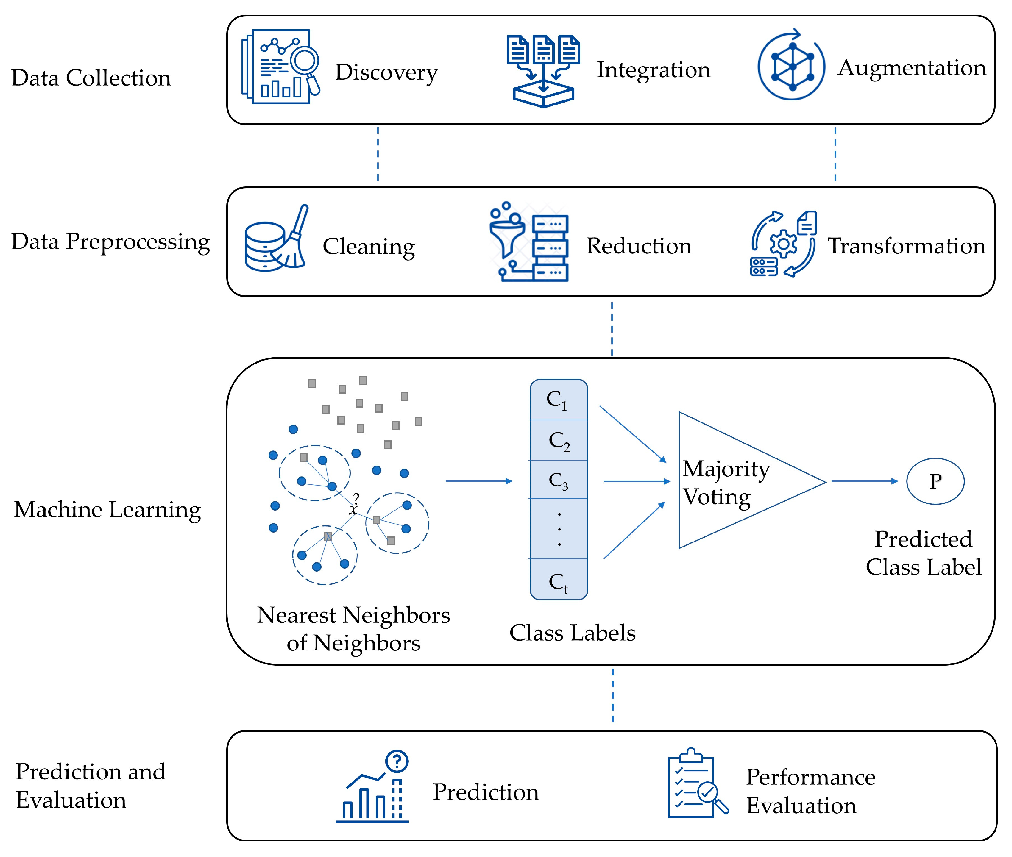
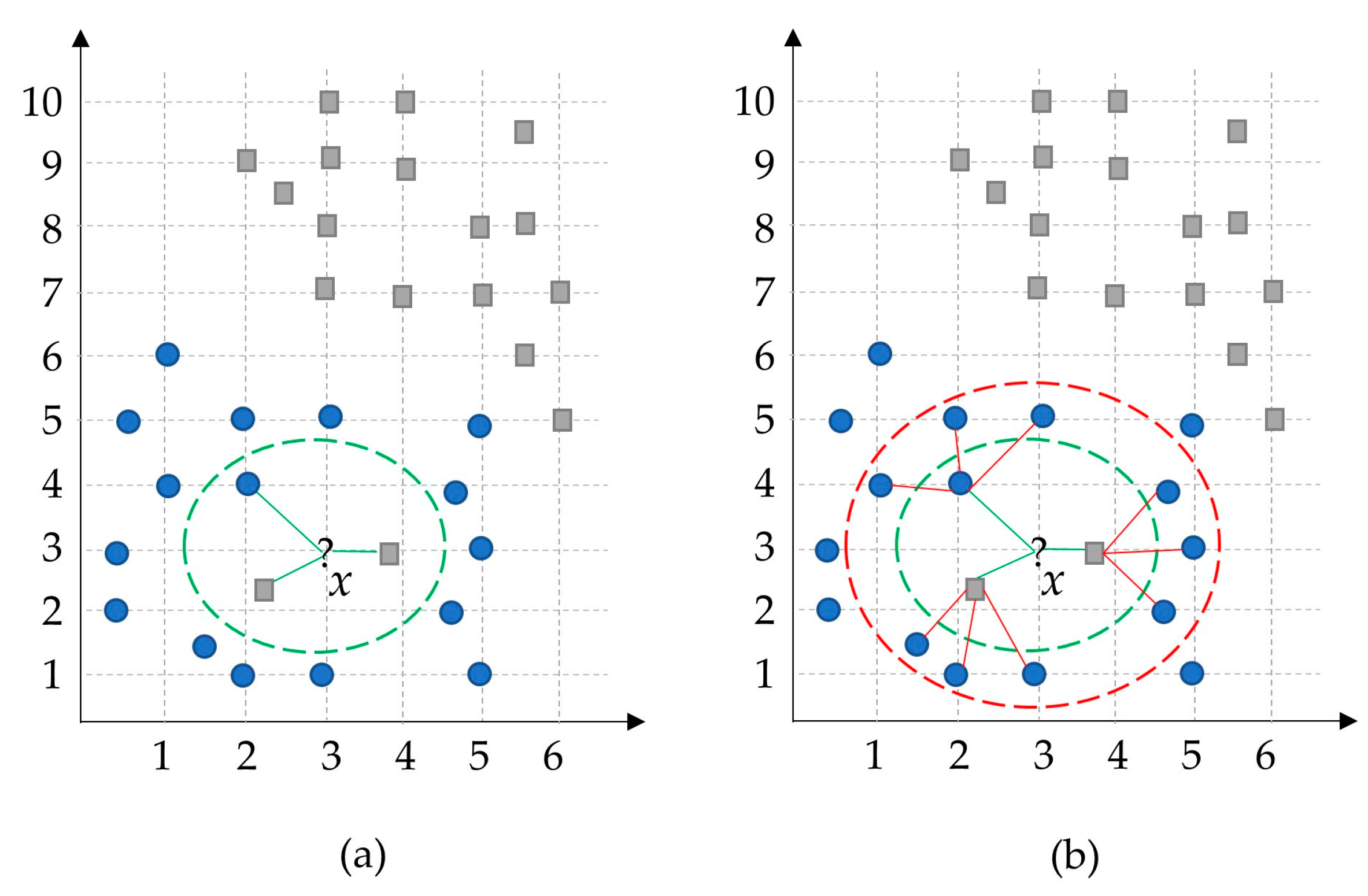
Our work is different from the previous studies in many respects. It presents a novel machine learning method, abbreviated as HLKNN. It proposes a different neighborhood searching mechanism. Instead of only considering k neighbors of a given query instance, it also takes into account the neighbors of these neighbors. It contributes to improving the accuracy of KNN and also other variants of the KNN algorithm in the literature.

3. Materials and Methods

3.1. The Proposed Method: High-Level K-Nearest Neighbors (HLKNN)

This section presents a comprehensive explanation of the High-Level K-Nearest Neighbors (HLKNN) method. Figure 1 presents the general structure of the proposed method. The first stage (the data collection stage) includes data discovery, data integration, and data augmentation. Data discovery involves gathering data from sources (i.e., databases) for analysis. Data integration refers to the process of combining datasets from different sources and provides the researcher with a unified view of these data. Data augmentation creates new sensible samples to increase the diversity and size of the training dataset while retaining its meaning. The next stage (the data preprocessing stage) consists of different steps such as data cleaning, data reduction, and data transformation. Data cleaning is performed by handling missing values and removing outlier observations. Data dimensionality reduction (i.e., feature selection) refers to using a method that identifies important variables and maps the samples from a high-dimensional space to a lower-dimensional space. Data transformation includes data smoothing, feature generation, and aggregation to convert the data into a form suitable for analysis. In the machine learning stage, a model is created by the proposed HLKNN method for categorizing the given input as an output class. For a given k value, the class labels of k-nearest neighbors are determined according to a distance metric such as Euclidean distance, Manhattan distance, or Minkowski distance. Afterward, the class labels of k-nearest neighbors of neighbors are added to the list. After that, a majority voting mechanism is applied to predict the output. This mechanism finds the label that achieves the highest number of votes in the list. For example, the winner of the list [c1 c1 c2 c2 c1] is determined as the class label “c1”. In the final stage, the categories of the test set samples are predicted, and evaluation metrics (i.e., accuracy, precision, recall, f-score) are used to assess the efficiency and robustness of the model.
Figure 2 illustrates an example of the proposed method. Assume that the number of neighbors is set to three (k = 3). Therefore, the classical KNN method will find the three closest neighbors of the given input sample x and select the square-gray class with the most votes. However, in the general view, it is expected to be classified the data point x as a blue-circle class. To solve this problem, our HLKNN method also considers the class labels of neighbors of these neighbors. In this case, the dominant class label in the list is determined as a blue circle. Thus, the proposed method handles the noisy observations in an efficient way during the classification task compared to the classical KNN method, which suffers from noise samples. The green dashed line denotes the low-level neighborhood, while the red dashed line indicates the high-level neighborhood.

3.2. Formal Description

Assume that D is a dataset with n samples such that   D = { x i , y i } i = 1 n . A data sample x i , y i consists of an m -dimensional input vector x i and its corresponding class y i . A class label y i is an element of a finite number of r different labels such that y i Y = { c 1 ,   c 1 ,   , c r } . Suppose a number k > 0 is fixed and denotes the number of neighbors. A KNN method basically depends on a distance metric d i s t :   R n × R n R such as the Euclidean distance measure. Given a query instance x , the neighborhood N k ( x ) in D is defined as the set of k samples x , where d i s t ( x , x ) is smallest.
Let L be a lazy learning algorithm, which takes a dataset   D = { x i , y i } i = 1 n and a query instance x as input and returns a class label y as output. The model M = L ( D ) is a function M : X Y that maps a query input x X to a class label y Y . The algorithm searches the k nearest points and selects the most frequent class among them.
For the classification, we propose a two-level KNN search to avoid noisy samples. First, the KNNs to x are computed for a query instance x D , so that the results are returned, building the set C . Next, the KNNs to each data sample s in C are computed and added in set C . The result of classification is determined by selecting the class label with the most votes.
Definition 1
(Low-Level Neighborhood). For a given query instance x , d i s t k ( x ) is the distance of the k th-nearest neighbor of x . For a given positive number k , the low-level neighborhood of x , which is denoted by N k ( x ) , contains every sample x whose distance from x is not greater than k th distance, such as
N k x = { x | x D   a n d   d i s t ( x , x ) d i s t k ( x ) }
Although the d i s t k ( x ) is well defined for a positive integer k , the cardinality of N k ( x ) can be greater than k . For instance, if there are 2 samples for 1-distance from test instance   x  and 1 sample for 2-distance from the instance, then, the cardinality of the low-level neighborhood will be 3 such that | N k x | = 3 , which is greater than the value of k = 2 .
Definition 2
(High-Level Neighborhood). The high-level neighborhood of a query instance x is the set N N k s for s N k ( x ) that contains k nearest neighbors of the neighbors of x .
The pseudocode of the HLKNN method is given in Algorithm A1 in the Appendix A section of this paper. The steps of the algorithm are explained in detail as follows.
Step 1: The algorithm utilizes the KNN search procedure to find k -nearest neighbors N k ( x ) of an instance x from the test set   D T e s t .
Step 2: Class labels are inserted into the list, named C , for each neighbor sample s in the set of neighbors N k ( x ) (low-level neighborhood). N N k ( s ) refers to the high-level neighborhood, which means the set of k -nearest neighbors of the neighbors.
Step 3: After specifying the high-level neighbors, class labels of the new set are added to the list.
Step 4: A voting mechanism is applied to predict the class label of the query instance   x .
Step 5: After producing an output for the instance   x , the whole process is repeated for other data instances in the testing set. In the end, the list   P   contains all predicted labels of the testing set.
The time complexity of HLKNN is O ( n ( k + k 2 ) ) since it calculates the distance from the query instance to each sample inside the dataset and determines ( k + k 2 ) nearest neighbors, where n is the number of instances in the dataset and k is the number of neighbors. For instance, for k from 1 to 7, the number of corresponding neighbors yielded 2, 6, 12, 20, 30, 42, and 56, respectively. According to our tests for various values of k, it was considered as 7 in the implementation of the HLKNN method in this study. Consequently, we assessed both KNN and HLKNN for 56 numbers of neighbors over 32 well-known datasets. We obtained 79.04% and 81.01% accuracy for the KNN and HLKNN methods on average, respectively. Although HLKNN involves additional processing time for handling neighbor–neighbor relationships, it has been developed to address the critical constraint of KNN, namely, noisy samples. Therefore, the emphasis is devoted to the reliability of the HLKNN method rather than execution time. The recent developments in high-performance computing enable us to take the edge off this limitation by permitting the parallel execution of the proposed approach.

4. Experimental Studies

This section presents the experiments performed to validate the effectiveness of the proposed method and discusses the main findings. The experimental studies were intended to put the outlined methodology into action, and benchmark datasets were used to validate the HLKNN method. By implementing the methodology, we aimed to provide insight into the contribution of the presented model.
The proposed method was implemented in the C# language using the Weka machine learning library [38,39]. To assess the performance, experiments were conducted by using the 10-fold cross-validation method. It should be noted here that we tested the HLKNN method by different values for the number of neighbors (known as   k ) and eventually determined the optimal value of 7.
To prove the efficiency of the proposed method, we applied it to 32 different widely used datasets. The validity of the proposed method was assessed by the various evaluation metrics, including accuracy, precision, recall, and f-score [40].
Accuracy refers to the number of correctly predicted data points to the total number of data points. In a more precise definition, it is calculated by dividing the sum of true positives and true negatives by the sum of true positives (TP), true negatives (TN), false positives (FP), and false negatives (FN). A true positive indicates a data point correctly classified as true, while a true negative is a data point correctly classified as false. Conversely, a false positive refers to a data point incorrectly classified as true, and a false negative is a data point incorrectly classified as false. The formula for calculating accuracy is expressed as Equation (2).
A c c u r a c y = T P + T N T P + T N + F P + F N
Precision is the proportion of relevant instances among all retrieved instances. In other words, it is determined by dividing the number of true positives by the total number of positive predictions (TP + FP), as represented in Equation (3).
P r e c i s i o n = T P T P + F P
Recall, referred to as sensitivity, is the fraction of retrieved instances among all relevant instances. It means that it measures the ratio of true positives to all the observations in the actual class, as given in Equation (4).
R e c a l l = T P T P + F N
The f-score is a metric that combines the precision and recall of the model, and it is calculated as the harmonic mean of the model’s precision and recall, as shown in Equation (5).
f - s c o r e =   2 P r e c i s i o n R e c a l l P r e c i s i o n + R e c a l l
This section is divided into three subsections: dataset description, results, and comparison with KNN variants, in which specific aspects of our research are explained in detail.

4.1. Dataset Description

The effectiveness of the proposed method was demonstrated through experimental studies using a specific set of datasets. The study involved 32 different benchmark datasets broadly used in machine learning, each well known, and publicly available. Table 1 provides details on these datasets, including the number of attributes, instances, classes, and domains. These datasets include a number of instances ranging from 36 to 45,211, attributes ranging from 2 to 45, and classes ranging from 2 to 10. They have different types of values, including numerical, categorical, or mixed type.
The datasets were obtained from the UCI Machine Learning Repository [41], covering various domains such as health, psychology, banking, environment, biology, and so on. The utilization of diverse datasets from different domains showcases the independence of the proposed approach from any specific field.

4.2. Results

To demonstrate the effectiveness of the HLKNN algorithm, we compared it with the standard KNN algorithm through the 10-fold cross-validation technique in terms of accuracy over 32 well-known datasets, which are described in Table 1. Table 2 shows the comparison results. According to the results, the proposed HLKNN method performed equal to or better than the standard KNN algorithm for 26 out of 32 datasets, which are marked in bold. For example, HLKNN showed better performance than KNN in the habermans-survival dataset with accuracy values of 74.84% and 72.55%, respectively. In another instance, HLKNN (95.52%) demonstrated its superiority over KNN (94.94%) in the wine dataset. In addition, HLKNN outperformed KNN on average, with accuracy values of 81.01% and 79.76%, respectively.
Since the HLKNN method includes the neighbors of neighbors, it does not encounter the risk of overfitting for noisy nearest instances in the dataset, and therefore better results can be revealed in comparison with the KNN method, as shown in Table 2. Actually, HLKNN is proposed for conquering the noise problem in the datasets. To avoid overfitting, it should be noted here that the value of k can be optimally determined by considering the data size, i.e., a low k value for small datasets.
During the evaluation process, the 10-fold cross-validation technique was used in this study. This technique involves randomly dividing the data into 10 equal-sized and disjoint partitions. During each iteration, one partition is kept for the test process, whereas the remaining partitions are used for the training task. The procedure is repeated 10 times, each time with different training/testing sets, and the overall evaluation metrics were calculated as the average of all 10 runs. Table 3 shows the ability of the HLKNN classifier fold by fold. The final column in the table reports the average accuracy of the 10-fold results. For example, accuracy values in each fold are not less than 86% in the banana dataset. Accuracy values range between 86.06% and 90.49% in the bank-marketing dataset. For instance, there are small fluctuations in the accuracy rates of the folds for the seismic-bumps dataset.
Accuracy alone is insufficient to evaluate a classifier’s performance. Therefore, besides accuracy, the KNN and HLKNN algorithms were also compared in terms of precision, recall, and f-score metrics. The formulas of the metrics are discussed in the experimental studies section. These metrics have values ranging from 0 to 1, where 1 is the best value. In other words, the performance improves as the value increases. The results obtained for each metric are shown in Figure 3, Figure 4, and Figure 5, respectively.
Figure 3 shows the comparison of the performances of algorithms in terms of precision. HLKNN achieved high precision values (above 0.95) for some datasets, including banknote-authentication, dermatology, iris, and wine. As can be seen from the figure, the outperformance of HLKNN over KNN was approved by the precision metric for 29 out of 32 datasets. This means that the HLKNN algorithm frequently tends to produce better results than the KNN algorithm. Moreover, notable differences between the results for the algorithms were observed for some datasets such as the pasture, planning-relax, and wholesale-region datasets. For example, HLKNN (0.9196) performed better than KNN (0.8483) in the sponge dataset with a remarkable difference in terms of precision metric. The biggest difference in the precision values of HLKNN and KNN was observed in the postoperative.patient.data dataset as 0.7111 and 0.5057, respectively. On average, HLKNN (0.8129) performed better than KNN (0.7611) with an improvement of over 5%.
Figure 4 shows the comparison of KNN and the proposed HLKNN method in terms of recall. The results from the figure revealed that HLKNN achieved equal or higher accuracy rates than KNN in 26 of 32 datasets. For example, in the saheart dataset, the recall value obtained by the HLKNN algorithm is closer to 1 than this obtained by the traditional KNN algorithm. As another instance, a notable difference between HLKNN and KNN was detected over the monks2 dataset in terms of recall metric. The biggest difference between the methods was observed on the planning-relax dataset with an improvement of over 8%. As can be seen, the best recall value (almost equal to 1) was obtained in the banknote-authentication dataset. HLKNN also achieved high recall values (above 0.95) for some datasets, including dermatology, iris, and wine.
Figure 5 shows the comparison of the performances of methods in terms of f-score. As can be seen, the outperformance of HLKNN over KNN was approved for 29 out of 32 datasets. For instance, HLKNN (0.9196) has better classification performance than KNN (0.8832) on the sponge dataset. Furthermore, it can be noted that there is a notable difference between the results for both algorithms in some datasets such as pasture, planning-relax, postoperative.patient.data, and wholesale-region. The best performance of the HLKNN method was achieved on the banknote-authentication dataset in terms of f-score value, which is almost equal to 1. On average, HLKNN (0.8111) performed better than KNN (0.7779) with an improvement of over 3%. According to the values of all metrics (accuracy, precision, recall, f-score), it can be concluded that HLKNN frequently tends to produce better results than KNN.

4.3. Comparison with KNN Variants

In this section, the proposed HLKNN method was compared with the variants of KNN [31,32,33,34,35,36,37] in terms of classification performance. Table 4 shows the results reported in the previous studies on the same datasets. Since the results were directly taken from the referenced studies, a range of popular datasets were regarded, including balance-scale, dermatology, ecoli, habermans-survival, heart, iris, liver-disorders, segment, and wine. The circumstances for datasets (i.e., data preprocessing) were not altered, to ensure a fair comparison in the same conditions between this study and the referenced studies. According to the results, the HLKNN outperformed the mentioned variants of KNN in all the datasets except the liver-disorders dataset. For example, HLKNN (86.03%) showed its superiority over uniform kNN [31] (81.47%), weighted kNN [31] (82.97%), and kNNGNN [31] (81.51%) on the ecoli dataset. As the results show, the HLKNN method acquired the highest accuracy of 97.33% for the iris dataset in comparison with other variants of KNN. In particular, the highest accuracy difference between HLKNN and the rest was observed in the wine dataset, where HLKNN increased the accuracy by over 26% against the k-MRS algorithm [32].

5. Conclusions and Future Work

In this paper, we proposed a machine learning model, named high-level k-nearest neighbors (HLKNN), to be utilized in predictive analytics. This model contributes to improving the classification ability of the KNN algorithm that is widely employed in various fields of machine learning. Since the KNN is sensitive to irrelevant data, its accuracy is adversely affected by the quality of the training dataset. According to the experimental results, our developed model usually outperformed KNN on popular datasets with average accuracy values of 81.01% and 79.76%, respectively. HLKNN performed equal to or better than KNN on 26 out of 32 datasets. Besides, the HLKNN method was compared with different types of KNN algorithms, namely, uniform kNN, weighted kNN, kNNGNN, k-MMS, k-MRS, k-NCN, NN, k-NFL, k-NNL, k-CNN, and k-TNN [31,32,33,34,35,36,37], which approved the superiority of the HLKNN method over other variants in terms of accuracy metric in different datasets, including balance-scale, dermatology, ecoli, habermans-survival, heart, iris, liver-disorders, segment, and wine.
The main outcomes of this study are summarized as follows:
  • The experimental results revealed the effectiveness of HLKNN compared to the KNN algorithm for 26 out of 32 datasets in terms of classification accuracy.
  • On average, the HLKNN outperformed KNN with accuracy values of 81.01% and 79.76%, respectively.
  • In terms of the precision metric, HLKNN (0.8129) performed better than KNN (0.7611) with an improvement of over 5% on average.
  • In terms of the recall metric, the results revealed that HLKNN achieved equal or higher accuracy rates than KNN in 26 of 32 datasets.
  • In terms of the f-score metric, HLKNN (0.8111) achieved better performance than KNN (0.7779) with an improvement of over 3% on average.
  • The proposed model in this study was also compared with various KNN-based methods, including uniform kNN, weighted kNN, kNNGNN, k-MMS, k-MRS, k-NCN, NN, k-NFL, k-NNL, k-CNN, and k-TNN, and the superiority of HLKNN over its counterparts was approved.
It is noteworthy to mention that the HLKNN method has several potential limitations. It is presented for classification tasks, not regression. Additionally, HLKNN depends on the existence of suitable neighbors of neighbors, in contrast to the original KNN method, which relies on only neighbors of a data point. In addition, HLKNN has a longer runtime compared to the KNN algorithm since it involves additional processing time for handling neighbor–neighbor relationships. We measured the runtime of both KNN and HLKNN over 32 well-known datasets by utilizing an Intel® system with properties of Core™ i7-8650U CPU 1.90 GHz and 8.00 GB memory. On average, we obtained runtimes of 0.31002 s and 2.60809 s, respectively, for the KNN and HLKNN algorithms. However, in comparison to the advantages (handling the noise problem, improving accuracy and generalization ability) of HLKNN, the drawback of higher computational cost can be reasonable in principle. Furthermore, in our study, the emphasis is given to the reliability of the methodology rather than running time. Moreover, the recent developments in high-performance computing permit alleviating this constraint by allowing the parallel execution of the proposed method. The main advantages and limitations of HLKNN contribute to making informed decisions on the model selection and implementation.
In future work, the HLKNN method can be applied to different datasets (e.g., sentiment analysis, human activity recognition, and predictive maintenance datasets) with different numbers of instances generated via real-world events or synthetically produced by artificial methods with the aim of achieving improved accuracies in terms of various evaluation metrics for a wide range of machine learning applications. In addition, it is conceivable to extend the HLKNN for the regression task with regard to various approaches, involving modifications of the model architecture, output interpretation, and data handling techniques.

Author Contributions

Conceptualization, E.O.K. and B.G.; methodology, D.B.; software, E.O.K., B.G. and D.B.; validation, E.O.K., B.G. and D.B.; formal analysis, E.O.K.; investigation, B.G.; resources, E.O.K. and B.G.; data curation, E.O.K. and B.G.; writing—original draft preparation, E.O.K. and B.G.; writing—review and editing, D.B.; visualization, E.O.K. and B.G.; supervision, D.B.; project administration, D.B.; funding acquisition, E.O.K. and D.B. All authors have read and agreed to the published version of the manuscript.

Funding

This research received no external funding.

Data Availability Statement

All datasets are publicly available in the UCI machine learning repository (https://archive.ics.uci.edu, accessed on 28 July 2023).

Conflicts of Interest

The authors declare no conflict of interest.

Abbreviations

The following abbreviations are used in this paper.
AIArtificial intelligence
BICSBlockchain-based integrity checking system
CSCCloud service consumers
CSPCloud service providers
DTRDecision tree regression
GISGeographical information systems
HBoFHybrid bag of features
HLKNNHigh-level k-nearest neighbors
IDSIntrusion detection system
KNNK-nearest neighbors
k-CNNK-center nearest neighbor
k-MMSK-min–max sum
k-MRSk-Min ranking sum
k-NCNK-nearest centroid neighborhood
k-NFLK-nearest feature line
k-NNGNNK-nearest neighbors learning method based on a graph neural network
k-NNLK-nearest neighbor line
k-TNNK-tunable nearest neighbor
LSTMLong short-term memory
MLMachine learning
NNNearest neighbor rule
PCAPrincipal component analysis
RFRandom forest
RSLRandom substance learning
SCSmart contract
SDNSoftware-defined network
SLAService level agreements
SVRSupport vector regression
UAVUnmanned aerial vehicles

Appendix A

Algorithm A1. High-Level K-Nearest Neighbors (HLKNN)
Inputs:
  DTrain: the training set with n data points
  DTest: test set
  k: the number of the nearest neighbors
Outputs:
  P: predicted labels for the testing set
Begin
  foreach x   DTest do
     N k ( x ) = kNearestNeighbors (DTrain, x, k)              # k-nearest neighbors of x
    C = Ø
    foreach s    N k ( x )  do
     y = Class (s)                              # class label of the low-level neighborhood
     C = C   y
      N N k ( s ) = kNearestNeighbors (DTrain, s, k)  # neighbors of the neighbors
     foreach o    N N k ( s )
      y = Class (o)                         # class label of the high-level neighborhood
      C = C  y
     end foreach
    end foreach
   c = a r g m a x y Y i : y = H i ( x ) t 1                            # prediction after the majority voting
    P = P c
  end foreach
End Algorithm

References

  1. Jiang, Y.; Li, X.; Luo, H.; Yin, S.; Kaynak, O. Quo Vadis Artificial Intelligence? Discov. Artif. Intell. 2022, 2, 629869. [Google Scholar] [CrossRef]
  2. Janiesch, C.; Zschech, P.; Heinrich, K. Machine Learning and Deep Learning. Electron. Mark. 2021, 31, 685–695. [Google Scholar] [CrossRef]
  3. Sarker, I.H. Machine Learning: Algorithms, Real-World Applications and Research Directions. SN Comput. Sci. 2021, 2, 160. [Google Scholar] [CrossRef] [PubMed]
  4. Han, J.; Pei, J.; Tong, H. Data Mining: Concepts and Techniques, 4th ed.; Morgan Kaufmann: Burlington, MA, USA, 2022. [Google Scholar]
  5. Ahmad, S.R.; Bakar, A.A.; Yaakub, M.R.; Yusop, N.M.M. Statistical validation of ACO-KNN algorithm for sentiment analysis. J. Telecommun. Electron. Comput. Eng. 2017, 9, 165–170. [Google Scholar]
  6. Kramer, O. Dimensionality Reduction with Unsupervised Nearest Neighbors; Springer: Berlin/Heidelberg, Germany, 2013; pp. 13–23. [Google Scholar]
  7. Hasan, M.J.; Kim, J.; Kim, C.H.; Kim, J.-M. Health State Classification of a Spherical Tank Using a Hybrid Bag of Features and K Nearest Neighbor. Appl. Sci. 2020, 10, 2525. [Google Scholar] [CrossRef]
  8. Beskopylny, A.N.; Stelmakh, S.A.; Shcherban, E.M.; Mailyan, L.R.; Meskhi, B.; Razveeva, I.; Chernilnik, A.; Beskopylny, N. Concrete Strength Prediction Using Machine Learning Methods CatBoost, k-Nearest Neighbors, Support Vector Regression. Appl. Sci. 2022, 12, 10864. [Google Scholar] [CrossRef]
  9. Wang, J.; Zhou, Z.; Li, Z.; Du, S. A Novel Fault Detection Scheme Based on Mutual k-Nearest Neighbor Method: Application on the Industrial Processes with Outliers. Processes 2022, 10, 497. [Google Scholar] [CrossRef]
  10. Lu, J.; Qian, W.; Li, S.; Cui, R. Enhanced K-Nearest Neighbor for Intelligent Fault Diagnosis of Rotating Machinery. Appl. Sci. 2021, 11, 919. [Google Scholar] [CrossRef]
  11. Salem, H.; Shams, M.Y.; Elzeki, O.M.; Abd Elfattah, M.; Al-Amri, J.F.; Elnazer, S. Fine-Tuning Fuzzy KNN Classifier Based on Uncertainty Membership for the Medical Diagnosis of Diabetes. Appl. Sci. 2022, 12, 950. [Google Scholar] [CrossRef]
  12. Miron, M.; Moldovanu, S.; Ștefănescu, B.I.; Culea, M.; Pavel, S.M.; Culea-Florescu, A.L. A New Approach in Detectability of Microcalcifications in the Placenta during Pregnancy Using Textural Features and K-Nearest Neighbors Algorithm. J. Imaging 2022, 8, 81. [Google Scholar] [CrossRef]
  13. Rattanasak, A.; Uthansakul, P.; Uthansakul, M.; Jumphoo, T.; Phapatanaburi, K.; Sindhupakorn, B.; Rooppakhun, S. Real-Time Gait Phase Detection Using Wearable Sensors for Transtibial Prosthesis Based on a kNN Algorithm. Sensors 2022, 22, 4242. [Google Scholar] [CrossRef]
  14. Nguyen, L.V.; Vo, Q.-T.; Nguyen, T.-H. Adaptive KNN-Based Extended Collaborative Filtering Recommendation Services. Big Data Cogn. Comput. 2023, 7, 106. [Google Scholar] [CrossRef]
  15. Corso, M.P.; Perez, F.L.; Stefenon, S.F.; Yow, K.-C.; García Ovejero, R.; Leithardt, V.R.Q. Classification of Contaminated Insulators Using k-Nearest Neighbors Based on Computer Vision. Computers 2021, 10, 112. [Google Scholar] [CrossRef]
  16. Syamsuddin, I.; Barukab, O.M. SUKRY: Suricata IDS with Enhanced kNN Algorithm on Raspberry Pi for Classifying IoT Botnet Attacks. Electronics 2022, 11, 737. [Google Scholar] [CrossRef]
  17. Derhab, A.; Guerroumi, M.; Gumaei, A.; Maglaras, L.; Ferrag, M.A.; Mukherjee, M.; Khan, F.A. Blockchain and Random Subspace Learning-Based IDS for SDN-Enabled Industrial IoT Security. Sensors 2019, 19, 3119. [Google Scholar] [CrossRef]
  18. Liu, G.; Zhao, H.; Fan, F.; Liu, G.; Xu, Q.; Nazir, S. An Enhanced Intrusion Detection Model Based on Improved kNN in WSNs. Sensors 2022, 22, 1407. [Google Scholar] [CrossRef] [PubMed]
  19. Zheng, Q.; Wang, L.; He, J.; Li, T. KNN-Based Consensus Algorithm for Better Service Level Agreement in Blockchain as a Service (BaaS) Systems. Electronics 2023, 12, 1429. [Google Scholar] [CrossRef]
  20. Fan, G.-F.; Guo, Y.-H.; Zheng, J.-M.; Hong, W.-C. Application of the Weighted K-Nearest Neighbor Algorithm for Short-Term Load Forecasting. Energies 2019, 12, 916. [Google Scholar] [CrossRef]
  21. Lee, C.-Y.; Huang, K.-Y.; Shen, Y.-X.; Lee, Y.-C. Improved Weighted k-Nearest Neighbor Based on PSO for Wind Power System State Recognition. Energies 2020, 13, 5520. [Google Scholar] [CrossRef]
  22. Gajan, S. Modeling of Seismic Energy Dissipation of Rocking Foundations Using Nonparametric Machine Learning Algorithms. Geotechnics 2021, 1, 534–557. [Google Scholar] [CrossRef]
  23. Martínez-Clark, R.; Pliego-Jimenez, J.; Flores-Resendiz, J.F.; Avilés-Velázquez, D. Optimum k-Nearest Neighbors for Heading Synchronization on a Swarm of UAVs under a Time-Evolving Communication Network. Entropy 2023, 25, 853. [Google Scholar] [CrossRef] [PubMed]
  24. Cha, G.-W.; Choi, S.-H.; Hong, W.-H.; Park, C.-W. Developing a Prediction Model of Demolition-Waste Generation-Rate via Principal Component Analysis. Int. J. Environ. Res. Public Health 2023, 20, 3159. [Google Scholar] [CrossRef]
  25. Bullejos, M.; Cabezas, D.; Martín-Martín, M.; Alcalá, F.J. A K-Nearest Neighbors Algorithm in Python for Visualizing the 3D Stratigraphic Architecture of the Llobregat River Delta in NE Spain. J. Mar. Sci. Eng. 2022, 10, 986. [Google Scholar] [CrossRef]
  26. Bullejos, M.; Cabezas, D.; Martín-Martín, M.; Alcalá, F.J. Confidence of a k-Nearest Neighbors Python Algorithm for the 3D Visualization of Sedimentary Porous Media. J. Mar. Sci. Eng. 2023, 11, 60. [Google Scholar] [CrossRef]
  27. Zhang, L.; Zhu, Y.; Su, J.; Lu, W.; Li, J.; Yao, Y. A Hybrid Prediction Model Based on KNN-LSTM for Vessel Trajectory. Mathematics 2022, 10, 4493. [Google Scholar] [CrossRef]
  28. Park, J.; Oh, J. Analysis of Collected Data and Establishment of an Abnormal Data Detection Algorithm Using Principal Component Analysis and K-Nearest Neighbors for Predictive Maintenance of Ship Propulsion Engine. Processes 2022, 10, 2392. [Google Scholar] [CrossRef]
  29. Tamamadin, M.; Lee, C.; Kee, S.-H.; Yee, J.-J. Regional Typhoon Track Prediction Using Ensemble k-Nearest Neighbor Machine Learning in the GIS Environment. Remote Sens. 2022, 14, 5292. [Google Scholar] [CrossRef]
  30. Mallek, A.; Klosa, D.; Büskens, C. Impact of Data Loss on Multi-Step Forecast of Traffic Flow in Urban Roads Using K-Nearest Neighbors. Sustainability 2022, 14, 11232. [Google Scholar] [CrossRef]
  31. Kang, S. k-Nearest Neighbor Learning with Graph Neural Networks. Mathematics 2021, 9, 830. [Google Scholar] [CrossRef]
  32. Mazón, J.N.; Micó, L.; Moreno-Seco, F. New Neighborhood Based Classification Rules for Metric Spaces and Their Use in Ensemble Classification. In Proceedings of the IbPRIA 2007 on Pattern Recognition and Image Analysis, Girona, Spain, 6–8 June 2007; pp. 354–361. [Google Scholar] [CrossRef]
  33. Sánchez, J.S.; Pla, F.; Ferri, F.J. On the Use of Neighbourhood-Based Non-Parametric Classifiers. Pattern Recognit. Lett. 1997, 18, 1179–1186. [Google Scholar] [CrossRef]
  34. Duda, R.O.; Hart, P.E.; Stork, D.G. Pattern Classification, 2nd ed.; John Wiley & Sons: New York, NY, USA, 2007; pp. 1–654. [Google Scholar] [CrossRef]
  35. Orozco-Alzate, M.; Castellanos-Domínguez, C.G. Comparison of the Nearest Feature Classifiers for Face Recognition. Mach. Vis. Appl. 2006, 17, 279–285. [Google Scholar] [CrossRef]
  36. Lou, Z.; Jin, Z. Novel Adaptive Nearest Neighbor Classifiers Based on Hit-Distance. In Proceedings of the 18th International Conference on Pattern Recognition (ICPR’06), Hong Kong, China, 20–24 August 2006; pp. 87–90. [Google Scholar] [CrossRef]
  37. Altiņcay, H. Improving the K-Nearest Neighbour Rule: Using Geometrical Neighbourhoods and Manifold-Based Metrics. Expert Syst. 2011, 28, 391–406. [Google Scholar] [CrossRef]
  38. Witten, I.H.; Frank, E.; Hall, M.A. Data Mining: Practical Machine Learning Tools and Techniques, 3rd ed.; Morgan Kaufmann: Cambridge, MA, USA, 2016; pp. 1–664. [Google Scholar]
  39. Aha, D.; Kibler, D. Instance-based learning algorithms. Mach. Learn. 1991, 6, 37–66. [Google Scholar] [CrossRef]
  40. Nica, I.; Alexandru, D.B.; Crăciunescu, S.L.P.; Ionescu, Ș. Automated Valuation Modelling: Analysing Mortgage Behavioural Life Profile Models Using Machine Learning Techniques. Sustainability 2021, 13, 5162. [Google Scholar] [CrossRef]
  41. Kelly, M.; Longjohn, R.; Nottingham, K. The UCI Machine Learning Repository. Available online: https://archive.ics.uci.edu (accessed on 28 July 2023).
Figure 1. The general structure of the proposed method.
Electronics 12 03828 g001
Figure 2. A sample simulation of the presented HLKNN method. (a) low-level neighborhood; (b) high-level neighborhood. (?, circle, square, red and green dot boxes, and lines mean what are the neighbors of an instance point x, a specific class of instances, another specific class of instances, boundaries to show high-level neighborhood and low-level neighborhood, and belonging of neighbors to an instance point, respectively)
Electronics 12 03828 g002
Figure 3. Comparison of the KNN and HLKNN algorithms on 32 benchmark datasets in terms of precision metric.
Electronics 12 03828 g003
Figure 4. Comparison of the KNN and HLKNN algorithms on 32 benchmark datasets in terms of recall metric.
Electronics 12 03828 g004
Figure 5. Comparison of the KNN and HLKNN algorithms on 32 benchmark datasets in terms of f-score metric.
Electronics 12 03828 g005
Table 1. Dataset characteristics.
IDDataset NameNumber of AttributesNumber of InstancesNumber of ClassesMissingDomain
1balance-scale46253Yespsychology
2banana253002Noshape
3bank-marketing1645,2112Nobanking
4banknote-authentication413722Nofinance
5blood-transfusion-service47482Nohealth
6climate-simulation-crashes175402Noenvironment
7credit-approval156902Yesfinance
8dermatology333666Yeshealth
9ecoli73368Yesbiology
10flare21010662Yesenvironment
11habermans-survival33062Yeshealth
12heart132702Yeshealth
13heart-disease-processed-cleveland133035Nohealth
14heart-disease-reprocessed-hungarian132945Nohealth
15horse-colic-surgical273682Yesanimal
16indian-liver-patient105832Nohealth
17iris41503Nolife
18led7digit750010Noscience
19liver-disorders63452Yeshealth
20monks266012Noscience
21pasture22363Noenvironment
22planning-relax131822Nohealth
23postoperative.patient.data8903Yeshealth
24saheart94622Nohealth
25segment1923107Noscience
26seismic-bumps1825842Nogeology
27sponge45763Yesmarine
28thoracic-surgery164702Nohealth
29vertebra-column-2c63102Nohealth
30vertebra-column-3c63103Nohealth
31wholesale-region84403Nobusiness
32wine131783Nochemistry
Table 2. Comparison of the KNN and HLKNN algorithms on 32 benchmark datasets in terms of classification accuracy (%) with equal and greater numbers in bold for each row.
Dataset NameKNNHLKNN
balance-scale89.4489.29
banana89.7589.40
bank-marketing88.5288.72
banknote-authentication99.8599.85
blood-transfusion-service77.1477.01
climate-simulation-crashes91.3091.48
credit-approval86.6786.67
dermatology96.1796.44
ecoli86.9086.03
flare281.9982.37
habermans-survival72.5574.84
heart81.9782.69
heart-disease-processed-cleveland59.7460.37
heart-disease-reprocessed-hungarian64.6366.69
horse-colic-surgical80.6781.33
indian-liver-patient67.5867.90
iris96.6797.33
led7digit73.6074.80
liver-disorders61.1662.61
monks258.4065.41
pasture66.6770.00
planning-relax62.6470.73
postoperative.patient.data71.1171.11
saheart64.2969.48
segment94.8994.28
seismic-bumps93.2793.31
sponge92.1191.96
thoracic-surgery84.6884.89
vertebra-column-2c79.0380.65
vertebra-column-3c76.1377.42
wholesale-region67.9571.59
wine94.9495.52
Mean79.7681.01
Table 3. Evaluation of HLKNN algorithm on 32 benchmark datasets in terms of classification accuracy (%) fold by fold (F stands for fold).
Dataset NameF1F2F3F4F5F6F7F8F9F10Mean
balance-scale90.4884.1380.9588.8995.2487.1098.3990.3287.1090.3289.29
banana90.0090.9488.6888.1191.7086.9888.6890.9488.3089.6289.40
bank-marketing90.0788.9487.6189.1687.6189.3886.0690.4989.1688.7288.72
banknote-authentication100.00100.00100.00100.0099.27100.0099.27100.00100.00100.0099.85
blood-transfusion-service74.6776.0081.3376.0080.0074.6776.0076.0077.0378.3877.01
climate-simulation-crashes92.5992.5992.5990.7494.4488.8990.7490.7492.5988.8991.48
credit-approval85.5186.9673.9186.9684.0692.7588.4184.0694.2089.8686.67
dermatology94.5997.30100.0097.3097.3094.59100.0097.2297.2288.8996.44
ecoli85.2985.2991.1879.4185.2982.3590.9190.9181.8287.8886.03
flare285.0584.1185.0581.3181.3177.5784.9185.8582.0876.4282.37
habermans-survival74.1983.8780.6574.1970.9764.5280.0080.0066.6773.3374.84
heart86.6780.0080.0073.3379.3196.5582.7686.2168.9793.1082.69
heart-disease-processed-cleveland64.5264.5261.2953.3360.0043.3356.6776.6756.6766.6760.37
heart-disease-reprocessed-hungarian76.6763.3360.0060.0086.2168.9758.6258.6279.3155.1766.69
horse-colic-surgical80.0070.0090.0080.0080.0083.3383.3390.0076.6780.0081.33
indian-liver-patient67.8069.4977.9772.4160.3465.5274.1462.0755.1774.1467.90
iris100.00100.0093.33100.00100.00100.00100.0093.3393.3393.3397.33
led7digit78.0070.0084.0070.0070.0068.0076.0078.0084.0070.0074.80
liver-disorders65.7157.1462.8657.1468.5747.0670.5967.6564.7164.7162.61
monks255.7465.0060.0073.3361.6773.3376.6760.0063.3365.0065.41
pasture75.0050.0025.00100.0075.0075.00100.0066.6766.6766.6770.00
planning-relax94.7473.6866.6738.8977.7872.2266.6788.8950.0077.7870.73
postoperative.patient.data77.7877.7855.5688.8944.4455.5666.6777.78100.0066.6771.11
saheart63.8376.6063.0460.8769.5767.3973.9171.7478.2669.5769.48
segment91.7796.1093.9491.3494.3794.8195.2496.1095.2493.9494.28
seismic-bumps93.0591.1295.3793.4491.8694.1992.2593.8093.8094.1993.31
sponge100.00100.00100.0075.00100.0087.5085.7185.7185.71100.0091.96
thoracic-surgery87.2382.9885.1187.2378.7287.2380.8587.2382.9889.3684.89
vertebra-column-2c77.4267.7470.9787.1080.6590.3277.4287.1077.4290.3280.65
vertebra-column-3c80.6567.7467.7480.6580.6590.3267.7480.6574.1983.8777.42
wholesale-region68.1875.0077.2765.9170.4559.0981.8277.2765.9175.0071.59
wine100.00100.0088.8994.4483.3394.44100.00100.00100.0094.1295.52
Table 4. Comparison of the proposed method and various KNN variants in terms of accuracy (%) with the greatest number in bold for each row.
Dataset NameUniformWeightedkNN
kNNkNNGNNk-MMSk-MRSk-NCNNNk-NFLk-NNLk-CNNk-TNNHLKNN
[31][31][31][32][32][33][34][35][36][37][37](Proposed)
balance-scale85.4785.6486.73--------89.29
dermatology---85.0885.6889.8985.6895.3693.3495.0390.7796.44
ecoli81.4782.9781.51--------86.03
habermans-survival---73.1473.9972.9468.2572.4264.7274.3173.0774.84
heart79.1979.0778.7463.3664.2967.3959.6767.7964.2966.4764.7582.69
iris91.1492.3494.2794.5395.2096.2795.2096.1393.7395.0796.2797.33
liver-disorders---66.1566.3269.2861.6367.3659.8363.4866.0962.61
segment89.7991.692.51--------94.28
wine89.6591.3994.7869.6368.7571.2271.5785.8483.3677.2869.8695.52
Disclaimer/Publisher’s Note: The statements, opinions and data contained in all publications are solely those of the individual author(s) and contributor(s) and not of MDPI and/or the editor(s). MDPI and/or the editor(s) disclaim responsibility for any injury to people or property resulting from any ideas, methods, instructions or products referred to in the content.

