Research and Hardware Implementation of a Reduced-Latency Quadruple-Precision Floating-Point Arctangent Algorithm

Abstract

In the field of digital signal processing, such as in navigation and radar, a significant number of high-precision arctangent function calculations are required. Lookup tables, polynomial approximation, and single/double-precision floating-point Coordinate Rotation Digital Computer (CORDIC) algorithms are insufficient to meet the demands of practical applications, where both high precision and low latency are essential. In this paper, based on the concept of trading area for speed, a four-step parallel branch iteration CORDIC algorithm is proposed. Using this improved algorithm, a 128-bit quad-precision floating-point arctangent function is designed, and the hardware circuit implementation of the arctangent algorithm is realized. The results demonstrate that the improved algorithm can achieve 128-bit floating-point arctangent calculations in just 32 cycles, with a maximum error not exceeding $2\times {10}^{-34}$ rad. It possesses exceptionally high computational accuracy and efficiency. Furthermore, the hardware area of the arithmetic unit is approximately 0.6317 mm${}^2$, and the power consumption is about 40.6483 mW under the TSMC 65 nm process at a working frequency of 500 MHz. This design can be well suited for dedicated CORDIC processor chip applications. The research presented in this paper holds significant value for high-precision and rapid arctangent function calculations in radar, navigation, meteorology, and other fields.

1. Introduction

With the rapid development of information technology, scientific computing has permeated almost all fields of science and engineering, finding extensive applications in energy surveys, game rendering, meteorology and oceanography, finance and insurance, and computer-aided design, among others. Scientific computing in these fields often involves a considerable number of floating-point transcendental function computations, such as trigonometric functions (sine and cosine), inverse tangent functions, exponential functions, etc. These functions cannot be directly represented and computed using a finite number of basic mathematical operations, such as addition, subtraction, multiplication, division, and square root. Instead, they require mathematical transformations or iterative approximation methods to obtain approximate results. Moreover, different domains have varying requirements for numerical precision during the computation process. In modern digital communication systems, common modulation techniques like orthogonal frequency-division multiplexing and quadrature amplitude modulation use signal phase as a modulation parameter, making phase extraction techniques increasingly important. Phase detection can be achieved using the arctangent function. Additionally, arctangent calculations are frequently encountered in applications such as digital frequency modulation and demodulation, navigation communication, motor control, and image processing. As their applications become more widespread, there is an increasing demand to efficiently and accurately implement floating-point arctangent functions in hardware. Previously, the main focus of optimizing floating-point arctangent was at the software level, aiming to enhance operational efficiency through code optimization. Over time, significant progress has been made in software optimization efforts, but it has now reached a point of diminishing returns, with limited room for further improvement. Conversely, hardware-level optimization offers more significant potential for improvement compared to software. Utilizing hardware for calculating transcendental functions like arctangent will consume a certain amount of chip area, but it significantly enhances computational efficiency. With the advancement of IC manufacturing processes, the benefits of hardware-level optimization undoubtedly outweigh the drawbacks.

Compared to the software level, the computation of the arctangent function is not easily implementable in hardware. There are no simple function modules that can be directly called; instead, hardware algorithms for the corresponding complex functions must be designed. In the early hardware algorithms, the main methods used for function computation were lookup tables [1,2] and polynomial approximation [3,4]. The principle of lookup tables is straightforward, where input values correspond one-to-one with the computed results of transcendental functions. The hardware structure can be simple and easily implemented within a small range of angle values [5]. However, when computing large angle values, a substantial amount of storage units is required, leading to inefficient resource utilization. On the other hand, the principle of polynomial approximation involves expanding the target function into a Taylor series within its domain, transforming the transcendental function into a series of power exponents, and approximating the function values numerically. But the use of Taylor series expansions involves a significant amount of multiplication and division, resulting in a large consumption of hardware resources [6]. Moreover, in order to accelerate computation speed, polynomial approximation often utilizes fourth or fifth-order Taylor series convergence, leading to insufficient precision due to the limitations of the order. Later, a combined approach that combines lookup tables with polynomial approximation was proposed [7]. This method effectively improves the efficiency of transcendental function computation, resulting in shorter operational cycles for the entire system. However, it requires the design of dedicated multipliers and adders, leading to a substantial increase in hardware circuit complexity and a significant increase in chip area. In summary, the aforementioned methods have drawbacks such as low computational efficiency, complex hardware resource requirements, and low computational precision.

To address the aforementioned issues, the Coordinate Rotation Digital Computer (CORDIC) algorithm was proposed in Reference [8]. This algorithm approximates the target angle by rotating a predetermined fixed angle repeatedly. Since the fixed rotation angle is only dependent on the base and the number of rotations, computations of complex functions can be decomposed into simple shift and addition operations [9]. Furthermore, the output precision of CORDIC is directly related to the number of iterations, offering adjustable output precision and a simple hardware implementation. To extend the range of basic functions that can be resolved, the unified CORDIC algorithms were introduced in Reference [10], unifying circular, hyperbolic, and linear rotations into the same CORDIC iteration equation. This laid a solid theoretical foundation for designing a versatile CORDIC processor. In recent years, numerous researchers have made significant efforts to improve CORDIC algorithms by enhancing computational accuracy, expanding angle coverage, reducing the number of iterations, and minimizing resource consumption. In Reference [11], a new micro-rotation angle set was used to achieve faster convergence and reduce the number of adders. However, its hardware implementation was challenging and did not achieve the desired precision. In Reference [12], the TCORDIC algorithm was proposed, combining low-latency CORDIC with Taylor algorithms, utilizing sign prediction, compressed iteration, and parallel iteration techniques to reduce latency and errors at the boundary. However, it increased power consumption and area usage. In Reference [13], the addition and subtraction operations in the CORDIC algorithm were executed in parallel using dedicated adders and subtractors, reducing latency but increasing resource consumption. In Reference [14], a hardware implementation method that divides resources between addition and subtraction operations was proposed, but it added hardware overhead and latency. Reference [15] presented a radix-4 CORDIC algorithm using a pipelined architecture, effectively balancing latency and hardware complexity. In Reference [16], the number of CORDIC iterations and bit-width were chosen based on the relationship derived from software-based simulation, reducing area and latency. However, its maximum operating frequency was limited, and precision was not improved. In Reference [17], an efficient CORDIC architecture based on the Ladner Fischer adder was proposed, but it consumed a significant amount of resources and was challenging to implement. In Reference [18], an approximation and lookup table strategy were utilized to increase data throughput but resulted in increased circuit area. In Reference [19], a scheme with dual-iteration sign prediction and multiplexer compression was proposed to reduce latency and control area, but precision improvement was not achieved. In Reference [20], a new hybrid algorithm for sine and cosine functions minimized the number of steps, reducing hardware volume and potential computation delay but significantly increasing the occupied ROM area. Reference [21] proposed a two-step branch CORDIC algorithm, where two branches execute different operations at each step, reducing computation cycles compared to the traditional CORDIC algorithm. In Reference [22], a CORDIC algorithm with rotation gain compensation was introduced, achieving a good trade-off between approximation error and resource consumption. However, its gain compensation had constant errors, limiting the precision of the algorithm. In Reference [23], a prediction circuit was included to select the most suitable predefined angle for iteration, reducing the number of iterations, but it only focused on phase and did not consider amplitude, and the maximum displacement count remained unchanged. In Reference [24], the Z-path was transformed into a lookup table to reduce circuit area consumption, but it did not improve calculation accuracy and speed. In Reference [25], resource consumption was reduced using a rough approximation method based on the traditional CORDIC algorithm, but output precision was compromised. In Reference [26], angle interval folding, optimal predefined angle selection, and omission of certain predefined angles were employed to narrow the iteration range and unify vector rotation direction. This achieved low resource consumption and short computational cycles but lacked sufficient precision improvement. Reference [27] proposed a low-latency hybrid CORDIC algorithm, further optimizing the computation cycle, significantly reducing the number of iterations. The comparative outcomes of the aforementioned research findings are illustrated in

Table 1. The comparative outcomes of the aforementioned research findings.

Paper	[8]	[10]	[11]
	CORDIC appears	Unified CORDIC Algorithms	New micro-rotation angle set
	Simple calculation	Extended	Increased rate of convergence
	——	——	Complex circuit
	[12]	[15]	[16]
	TCORDIC	Radix-4 CORDIC	Software-assisted
	Low latency and error	Balanced latency and hardware	Reduced latency and area
	Large area	——	Poor accuracy
	[17]	[18]	[19]
Innovation	Ladner Fischer	Approximate calculation	Double symbol prediction
Advantage	Efficient	Improved throughput	Reduced latency
Disadvantage	Complex	Large area	Poor accuracy
	[21]	[22]	[23]
	Two-step branch CORDIC	Rotational gain compensation	Anticipation circuit
	Reduced latency	Balanced error and area	Reduced iterations
	Poor accuracy	Precision limitation	Complex
	[25]	[26]	[27]
	Rough approximation	Angular interval folding	Low latency hybrid CORDIC
	Less resource consumption	Short computing cycle	Reduced iterations
	Poor accuracy	Poor accuracy	——

.

From the analysis of the above literature, it can be observed that the current research on floating-point arctangent functions still exhibits drawbacks such as low computational precision, a high number of iterations, and slow execution efficiency. Moreover, to the best of our knowledge, there is currently no existing 128-bit floating-point arctangent arithmetic unit in this field. Therefore, these issues are addressed in this paper by studying the computational strategy for high-precision floating-point arctangent functions, thus filling the research gap in this area. The main contributions of this paper are as follows:

• An improved CORDIC algorithm is proposed, utilizing a four-step parallel branch iteration strategy to reduce the number of iterations in the arctangent algorithm and decrease the output latency;
• The improved CORDIC algorithm is applied to the calculation of a 128-bit high-precision floating-point arctangent function, resulting in improved computational precision while reducing computational complexity;
• The 128-bit high-precision floating-point arctangent algorithm is implemented in hardware, making it suitable for the design of dedicated chips for high-precision CORDIC algorithms.

The organization of this paper is as follows: In Section 2, the fundamental CORDIC algorithm is introduced and improved. A four-step parallel branch iteration CORDIC algorithm is proposed and applied to the calculation of a quad-precision floating-point arctangent function. In Section 3, the hardware circuit implementation and optimization of the quad-precision floating-point arctangent function are presented. In Section 4, the circuit simulation results are compared and analyzed with the standard calculations from Python’s bigfloat package, and FPGA and ASIC implementations of the hardware circuit are performed. Finally, conclusions are presented in Section 5.

2. CORDIC Algorithm and Improvement

2.1. IEEE 754 Floating-Point Standard

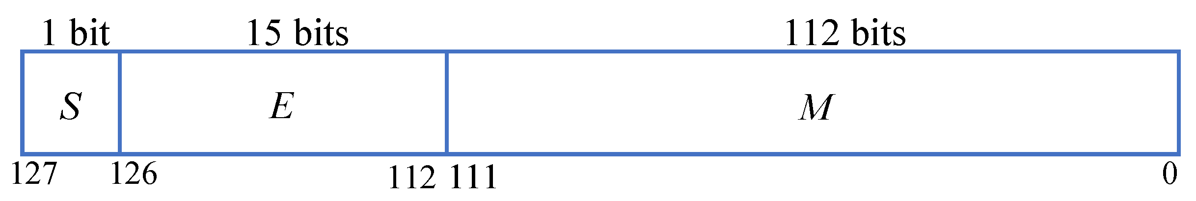
For floating-point computation, the Institute of Electrical and Electronics Engineers (IEEE) proposed the IEEE-754 floating-point standard in 1985, and the latest version was released in 2008 [28]. The IEEE-754 standard defines floating-point numbers as composed of three parts: the sign bit, exponent part, and mantissa part, represented in scientific notation as shown in Equation (1).

$${(-1)}^S\times 2^{E-bias}\times 1.M$$

(1)

Here, S represents the sign bit, E represents the value of the exponent part, bias is a fixed offset value, M represents the value of the mantissa part, and 1.M is the actual value used for computation, composed of the mantissa part value M and 1 hidden bit of precision. Floating-point numbers of different precisions have different bias values, as well as varying widths for the exponent and mantissa parts, resulting in different ranges for representing fixed-point numbers. The parameters of different precision floating-point numbers are shown in

Table 2. The composition of floating-point numbers of different precision.

Component	Float (32 bits)	Double (64 bits)	Quadruple-Precision (128 bits)
S	1 bit	1 bit	1 bit
E	8 bits	11 bits	15 bits
M	23 bits	52 bits	112 bits
Bias	127	1023	16,383

.

With the rapid development of integrated circuits, high-performance processors increasingly rely on high-speed and high-precision floating-point computations. Consequently, single-precision and double-precision floating-point calculations are no longer sufficient to meet the requirements. Therefore, this paper focuses on studying floating-point arctangent computation under quad-precision conditions. The format of normalized quad-precision floating-point numbers is illustrated in Figure 1.

Furthermore, based on the different values of E and M, IEEE-754 classifies floating-point numbers into various types, as shown in

Table 3. Floating-point numbers of different types.

Type	E	M	Comment
0	0	0	0 has a sign determined by the sign bit S
Subnormal	0	$\ne 0$	Supplement the precision bit with 0
∞	15’h7fff	0	${(-1)}^S\times \infty$
NaN	15’h7fff	$\ne 0$
Finite number	15’h0000 < E < 15’h7fff	1023	${(-1)}^S\times 2^{E-16383}\times 1.M$

. In the subsequent arctangent computation, it is essential to perform the detection and handling of exceptions and special inputs according to the specified floating-point number types listed here.

2.2. Basic CORDIC Algorithm

In Reference [8], the CORDIC algorithm was first proposed. Its principle involves rotating the initial vector in different directions by specific angle values within a given coordinate system to iteratively approach the target vector infinitely. In the polar coordinate system, the iterative formula of the CORDIC algorithm is given by Equation (2), where (X,Y,Z) represents the intermediate iteration values of the three channels, $\gamma$ is the rotation factor and $\gamma \in \{-1,1\}$, and it determines the rotation direction for each iteration. The value of $\gamma$ can be either 1 for counterclockwise rotation or −1 for clockwise rotation. ${\theta }_i$ represents the rotation angle for each iteration, satisfying Equation (3). During the hardware circuit implementation, each value of ${\theta }_i$ is pre-stored in a lookup table with a specific precision.

$$\left\{\begin{array}{c}{X}_{i+1}=X_i-{\gamma }_i{Y}_i{2}^{-i}\hfill \\ Y_{i+1}=Y_i+{\gamma }_i{X}_i{2}^{-i}\hfill \\ Z_{i+1}=Z_i-{\gamma }_i{\theta }_i\hfill \end{array}\right.$$

(2)

$${\theta }_i={tan}^{-1}{2}^{-i}$$

(3)

In vector mode, the goal of iteration is $Y\to 0$, which is to rotate the initial vector $(X_0,Y_0)$ to align with the x axis. Upon completion of the iteration, the final iteration values for the three channels are given by Equation (4). In this equation, $P_n$ represents the correction term during the iteration process, which satisfies Equation (5).

$$\left\{\begin{array}{c}{X}_n=\frac{1}{P_n}\sqrt{X_0^2+Y_0^2}\hfill \\ Y_n=0\hfill \\ Z_n=Z_0+{tan}^{-1}\left(\frac{Y_0}{X_0}\right)\hfill \end{array}\right.$$

(4)

$$P_n=\prod _{i=0}^{n-1}cos\left({tan}^{-1}{2}^{-i}\right)=\prod _{i=0}^{n-1}\frac{1}{\sqrt{1+{tan}^2{\theta }_i}}=\prod _{i=0}^{n-1}\frac{1}{\sqrt{1+2^{-2i}}}\approx 0.607253$$

(5)

Therefore, by initializing $(X_0,Y_0,Z_0)$ with the appropriate values $(x,y,0)$ for the three channels, the final values of Z at the end of the iteration represent the result of the arctangent function $arctan(y/x)$.

Through analysis, it can be observed that, for quad-precision floating-point number computations, the traditional CORDIC algorithm faces a bottleneck. This is because each iteration’s rotation factor needs to wait for the result of the previous iteration for prediction, limiting the algorithm to a single-step iteration. In other words, only one iteration can be performed in each clock cycle, yielding 1-bit precision. Consequently, to achieve 113-bit precision, it would require 113 clock cycles, resulting in slow computation speed. Therefore, the following sections focus on addressing this issue and proposing improvements to the traditional CORDIC algorithm.

2.3. Four-Step Parallel Branching Iteration CORDIC Algorithm for Four-Precision Floating-Point Arctangent Function

In order to address the issue of slow computation speed in the traditional CORDIC algorithm, a four-step parallel branching iterative CORDIC algorithm suitable for arctangent functions is proposed in this paper. The algorithm is designed by taking into account both the complexity of circuit design and the efficiency of computation.

Unlike the method in Equation (2) where each of the three channels $(X,Y,Z)$ undergoes only one iteration based on the rotation factor, we adopt the concept of trading area for time and serial to parallel conversion. By performing four iterations in parallel within one clock cycle, the overall computation efficiency is improved fourfold. Below is the derivation of the four-step parallel branching iterative formula for the three channels $(X,Y,Z)$. For channel X, after four iterations, we substitute the results into Equation (2) successively, leading to Equation (6):

$$\left\{\begin{array}{c}\begin{array}{cc}\hfill & X_{i+1}=X_i-{\gamma }_i{Y}_i{2}^{-i}\hfill \\ \hfill & X_{i+2}=X_{i+1}-{\gamma }_{i+1}{Y}_{i+1}{2}^{-(i+1)}\hfill \\ \hfill & =X_i-{\gamma }_i{Y}_i{2}^{-i}-{\gamma }_{i+1}{Y}_i{2}^{-(i+1)}-{\gamma }_{i+1}{\gamma }_i{X}_i{2}^{-(2i+1)}\hfill \\ \hfill & X_{i+3}=X_{i+2}-{\gamma }_{i+2}{Y}_{i+2}{2}^{-(i+2)}\hfill \\ \hfill & =X_{i+1}-{\gamma }_{i+1}{Y}_{i+1}{2}^{-(i+1)}-{\gamma }_{i+2}(Y_{i+1}+{\gamma }_{i+1}{X}_{i+1}{2}^{-(i+1)})2^{-(i+2)}\hfill \\ \hfill & =X_i-{\gamma }_i{Y}_i{2}^{-i}-{\gamma }_{i+1}(Y_i+{\gamma }_i{X}_i{2}^{-i})2^{-(i+1)}-{\gamma }_{i+2}[Y_i+{\gamma }_i{X}_i{2}^{-i}+{\gamma }_{i+1}(X_i-{\gamma }_i{Y}_i{2}^{-i})2^{-(i+1)}]2^{-(i+2)}\hfill \\ \hfill & =X_i-{\gamma }_i{Y}_i{2}^{-i}-{\gamma }_{i+1}{Y}_i{2}^{-(i+1)}-{\gamma }_{i+1}{\gamma }_i{X}_i{2}^{-(2i+1)}-{\gamma }_{i+2}{Y}_i{2}^{-(i+2)}\hfill \\ \hfill & -{\gamma }_{i+2}{\gamma }_i{X}_i{2}^{-(2i+2)}-{\gamma }_{i+2}{\gamma }_{i+1}{X}_i{2}^{-(2i+3)}+{\gamma }_{i+2}{\gamma }_{i+1}{\gamma }_i{Y}_i{2}^{-(3i+3)}\hfill \\ \hfill & X_{i+4}=\{1+{\gamma }_{i+3}{\gamma }_{i+2}{\gamma }_{i+1}{\gamma }_i{2}^{-(4i+6)}-[16{\gamma }_{i+1}{\gamma }_i+8{\gamma }_{i+2}{\gamma }_i+4({\gamma }_{i+2}{\gamma }_{i+1}+{\gamma }_{i+3}{\gamma }_i)\hfill \\ \hfill & +2{\gamma }_{i+3}{\gamma }_{i+1}+{\gamma }_{i+3}{\gamma }_{i+2}]2^{-(2i+5)}\}·X_i-[(8{\gamma }_i+4{\gamma }_{i+1}+2{\gamma }_{i+2}+{\gamma }_{i+3})2^{-(i+3)}\hfill \\ \hfill & -(8{\gamma }_{i+2}{\gamma }_{i+1}{\gamma }_i+4{\gamma }_{i+3}{\gamma }_{i+1}{\gamma }_i+2{\gamma }_{i+3}{\gamma }_{i+2}{\gamma }_i+{\gamma }_{i+3}{\gamma }_{i+2}{\gamma }_{i+1})2^{-(3i+6)}]·Y_i\hfill \end{array}\hfill \end{array}\right.$$

(6)

Similarly, for both channel Y and channel Z, Equations (7) and (8) can be derived.

$$\left\{\begin{array}{c}\begin{array}{cc}\hfill & Y_{i+1}=Y_i+{\gamma }_i{X}_i{2}^{-i}\hfill \\ \hfill & Y_{i+2}=Y_{i+1}+{\gamma }_{i+1}{X}_{i+1}{2}^{-(i+1)}\hfill \\ \hfill & =Y_i+{\gamma }_i{X}_i{2}^{-i}+{\gamma }_{i+1}{X}_i{2}^{-(i+1)}-{\gamma }_{i+1}{\gamma }_i{Y}_i{2}^{-(2i+1)}\hfill \\ \hfill & Y_{i+3}=Y_{i+2}+{\gamma }_{i+2}{X}_{i+2}{2}^{-(i+2)}\hfill \\ \hfill & =(Y_{i+1}+{\gamma }_{i+1}{X}_{i+1}{2}^{-(i+1)})+{\gamma }_{i+2}(X_{i+1}-{\gamma }_{i+1}{Y}_{i+1}{2}^{-(i+1)})2^{-(i+2)}\hfill \\ \hfill & =Y_{i+1}+[X_i-{\gamma }_i{Y}_i{2}^{-i}-{\gamma }_{i+1}(Y_i+{\gamma }_i{X}_i{2}^{-i})2^{-(i+1)}]{\gamma }_{i+2}{2}^{-(i+2)}+{\gamma }_{i+1}{X}_{i+1}{2}^{-(i+1)}\hfill \\ \hfill & =Y_i+{\gamma }_i{X}_i{2}^{-i}+{\gamma }_{i+1}{X}_i{2}^{-(i+1)}-{\gamma }_{i+1}{\gamma }_i{Y}_i{2}^{-(2i+1)}+{\gamma }_{i+2}{X}_i{2}^{-(i+2)}\hfill \\ \hfill & -{\gamma }_{i+2}{\gamma }_i{Y}_i{2}^{-(2i+2)}-{\gamma }_{i+2}{\gamma }_{i+1}{Y}_i{2}^{-(2i+3)}-{\gamma }_{i+2}{\gamma }_{i+1}{\gamma }_i{X}_i{2}^{-(3i+3)}\hfill \\ \hfill & Y_{i+4}=\{1+{\gamma }_{i+3}{\gamma }_{i+2}{\gamma }_{i+1}{\gamma }_i{2}^{-(4i+6)}-[16{\gamma }_{i+1}{\gamma }_i+8{\gamma }_{i+2}{\gamma }_i+4({\gamma }_{i+2}{\gamma }_{i+1}+{\gamma }_{i+3}{\gamma }_i)\hfill \\ \hfill & +2{\gamma }_{i+3}{\gamma }_{i+1}+{\gamma }_{i+3}{\gamma }_{i+2}]2^{-(2i+5)}\}·Y_i+[(8{\gamma }_i+4{\gamma }_{i+1}+2{\gamma }_{i+2}+{\gamma }_{i+3})2^{-(i+3)}\hfill \\ \hfill & -(8{\gamma }_{i+2}{\gamma }_{i+1}{\gamma }_i+4{\gamma }_{i+3}{\gamma }_{i+1}{\gamma }_i+2{\gamma }_{i+3}{\gamma }_{i+2}{\gamma }_i+{\gamma }_{i+3}{\gamma }_{i+2}{\gamma }_{i+1})2^{-(3i+6)}]·X_i\hfill \end{array}\hfill \end{array}\right.$$

(7)

$$\left\{\begin{array}{l}{Z}_{i+1}=Z_i-{\gamma }_i{\theta }_i\\ Z_{i+2}=Z_{i+1}-{\gamma }_{i+1}{\theta }_{i+1}=Z_i-{\gamma }_i{\theta }_i-{\gamma }_{i+1}{\theta }_{i+1}\\ Z_{i+3}=Z_{i+2}-{\gamma }_{i+2}{\theta }_{i+2}=Z_i-{\gamma }_i{\theta }_i-{\gamma }_{i+1}{\theta }_{i+1}-{\gamma }_{i+2}{\theta }_{i+2}\\ Z_{i+4}=Z_{i+3}-{\gamma }_{i+3}{\theta }_{i+3}=Z_i-({\gamma }_i{\theta }_i+{\gamma }_{i+1}{\theta }_{i+1}+{\gamma }_{i+2}{\theta }_{i+2}+{\gamma }_{i+3}{\theta }_{i+3})\end{array}\right.$$

(8)

Thus, we obtain the $(X_{i+4},Y_{i+4},Z_{i+4})$ of the three channels after each cycle iteration in the four-step parallel branch iteration algorithm. It can be observed that the key to successful iteration lies in accurately predicting the rotation factor $R_i=\{{\gamma }_i,{\gamma }_{i+1},{\gamma }_{i+2},{\gamma }_{i+3}\}$ simultaneously. According to formula (4), the CORDIC algorithm for arctangent aims to rotate vector $(X,Y)$ to the x axis, and the prediction of the ${\gamma }_i$ sign is determined by the sign bit $y_i$ from the previous iteration. In this algorithm, the value range of $R_i=\{{\gamma }_i,{\gamma }_{i+1},{\gamma }_{i+2},{\gamma }_{i+3}\}$ is determined as $\{0,-1\}$, where 0 indicates that after this iteration, the algorithm will cross the x axis without rotation, and −1 indicates that after this iteration, the algorithm will still not cross the x axis, requiring a clockwise rotation. Therefore, such value assignment ensures that $Z_{i+4}$ remains in the first quadrant, avoiding crossing the x axis, and it causes some coefficients in the expression of $(X_{i+4},Y_{i+4},Z_{i+4})$ to be 0, effectively reducing the algorithm’s complexity and saving hardware circuit area.

When the range of $R_i=\{{\gamma }_i,{\gamma }_{i+1},{\gamma }_{i+2},{\gamma }_{i+3}\}$ is considered to be $\{0,-1\}$, all its possible results fall within the range of $\{0,0,0,0\}$ to $\{-1,-1,-1,-1\}$. As for the iterative expression of $Y_{i+4}$, the potential outcomes of the 16 branches are shown in

Table 4. The 16 branches of channel Y.

${\mathit{R}}_{\mathit{i}}$	${\mathit{Y}}_{\mathit{i}+4}$
(0,0,0,0)	$Y_i$
(0,0,0,−1)	$Y_i$−$2^{-(i+3)}$$X_i$
(0,0,−1,0)	$Y_i$−$2^{-(i+2)}$$X_i$
(0,−1,0,0)	$Y_i$−$2^{-(i+1)}$$X_i$
(−1,0,0,0)	$Y_i$−$2^{-i}$$X_i$
(0,0,−1,−1)	(1−$2^{-(2i+5)}$)$Y_i$−3*$2^{-(i+3)}$$X_i$
(0,−1,0,−1)	(1−$2^{-(2i+4)}$)$Y_i$−5*$2^{-(i+3)}$$X_i$
(0,−1,−1,0)	(1−$2^{-(2i+3)}$)$Y_i$−6*$2^{-(i+3)}$$X_i$
(−1,0,0,−1)	(1−$2^{-(2i+3)}$)$Y_i$−9*$2^{-(i+3)}$$X_i$
(−1,0,−1,0)	(1−$2^{-(2i+2)}$)$Y_i$−10*$2^{-(i+3)}$$X_i$
(−1,−1,0,0)	(1−$2^{-(2i+1)}$)$Y_i$−12*$2^{-(i+3)}$$X_i$
(0,−1,−1,−1)	(1−7*$2^{-(2i+5)}$)$Y_i$−(7*$2^{-(i+3)}$−$2^{-(3i+6)}$)$X_i$
(−1,0,−1,−1)	(1−13*$2^{-(2i+5)}$)$Y_i$−(11*$2^{-(i+3)}$−$2^{-(3i+5)}$)$X_i$
(−1,−1,0,−1)	(1−22*$2^{-(2i+5)}$)$Y_i$−(13*$2^{-(i+3)}$−$2^{-(3i+4)}$)$X_i$
(−1,−1,−1,0)	(1−28*$2^{-(2i+5)}$)$Y_i$−(14*$2^{-(i+3)}$−$2^{-(3i+3)}$)$X_i$
(−1,−1,−1,−1)	(1−35*$2^{-(2i+5)}$+$2^{-(4i+6)}$)$Y_i$−(15*$2^{-(i+3)}$−15*$2^{-(3i+5)}$)$X_i$

. Completing these 16 branch computations requires a total of 32 additions and subtractions, 16 multiplications, and 21 shift operations.

The 16 potential branch results for the iterative expression of $X_{i+4}$ are shown in

Table 5. The 16 branches of channel X.

${\mathit{R}}_{\mathit{i}}$	${\mathit{X}}_{\mathit{i}+4}$
(0,0,0,0)	$X_i$
(0,0,0,−1)	$X_i$+$2^{-(i+3)}$$Y_i$
(0,0,−1,0)	$X_i$+$2^{-(i+2)}$$Y_i$
(0,−1,0,0)	$X_i$+$2^{-(i+1)}$$Y_i$
(−1,0,0,0)	$X_i$+$2^{-i}$$Y_i$
(0,0,−1,−1)	(1−$2^{-(2i+5)}$)$X_i$+3*$2^{-(i+3)}$$Y_i$
(0,−1,0,−1)	(1−$2^{-(2i+4)}$)$X_i$+5*$2^{-(i+3)}$$Y_i$
(0,−1,−1,0)	(1−$2^{-(2i+3)}$)$X_i$+6*$2^{-(i+3)}$$Y_i$
(−1,0,0,−1)	(1−$2^{-(2i+3)}$)$X_i$+9*$2^{-(i+3)}$$Y_i$
(−1,0,−1,0)	(1−$2^{-(2i+2)}$)$X_i$+10*$2^{-(i+3)}$$Y_i$
(−1,−1,0,0)	(1−$2^{-(2i+1)}$)$X_i$+12*$2^{-(i+3)}$$Y_i$
(0,−1,−1,−1)	(1−7*$2^{-(2i+5)}$)$X_i$+(7*$2^{-(i+3)}$−$2^{-(3i+6)}$)$Y_i$
(−1,0,−1,−1)	(1−13*$2^{-(2i+5)}$)$X_i$+(11*$2^{-(i+3)}$−$2^{-(3i+5)}$)$Y_i$
(−1,−1,0,−1)	(1−22*$2^{-(2i+5)}$)$X_i$+(13*$2^{-(i+3)}$−$2^{-(3i+4)}$)$Y_i$
(−1,−1,−1,0)	(1−28*$2^{-(2i+5)}$)$X_i$+(14*$2^{-(i+3)}$−$2^{-(3i+3)}$)$Y_i$
(−1,−1,−1,−1)	(1−35*$2^{-(2i+5)}$+$2^{-(4i+6)}$)$X_i$+(15*$2^{-(i+3)}$−15*$2^{-(3i+5)}$)$Y_i$

.

The 16 potential branch results for the iterative expression of $Z_{i+4}$ are shown in

Table 6. The 16 branches of channel Z.

${\mathit{R}}_{\mathit{i}}$	${\mathit{X}}_{\mathit{i}+4}$
(0,0,0,0)	$Z_i$
(0,0,0,−1)	$Z_i$+${\theta }_{i+3}$
(0,0,−1,0)	$Z_i$+${\theta }_{i+2}$
(0,−1,0,0)	$Z_i$+${\theta }_{i+1}$
(−1,0,0,0)	$Z_i$+${\theta }_i$
(0,0,−1,−1)	$Z_i$+${\theta }_{i+2}$+${\theta }_{i+3}$
(0,−1,0,−1)	$Z_i$+${\theta }_{i+1}$+${\theta }_{i+3}$
(0,−1,−1,0)	$Z_i$+${\theta }_{i+1}$+${\theta }_{i+2}$
(−1,0,0,−1)	$Z_i$+${\theta }_i$+${\theta }_{i+3}$
(−1,0,−1,0)	$Z_i$+${\theta }_i$+${\theta }_{i+2}$
(−1,−1,0,0)	$Z_i$+${\theta }_i$+${\theta }_{i+1}$
(0,−1,−1,−1)	$Z_i$+${\theta }_{i+1}$+${\theta }_{i+2}$+${\theta }_{i+3}$
(−1,0,−1,−1)	$Z_i$+${\theta }_i$+${\theta }_{i+2}$+${\theta }_{i+3}$
(−1,−1,0,−1)	$Z_i$+${\theta }_i$+${\theta }_{i+1}$+${\theta }_{i+3}$
(−1,−1,−1,0)	$Z_i$+${\theta }_i$+${\theta }_{i+1}$+${\theta }_{i+2}$
(−1,−1,−1,−1)	$Z_i$+${\theta }_i$+${\theta }_{i+1}$+${\theta }_{i+2}$+${\theta }_{i+3}$

.

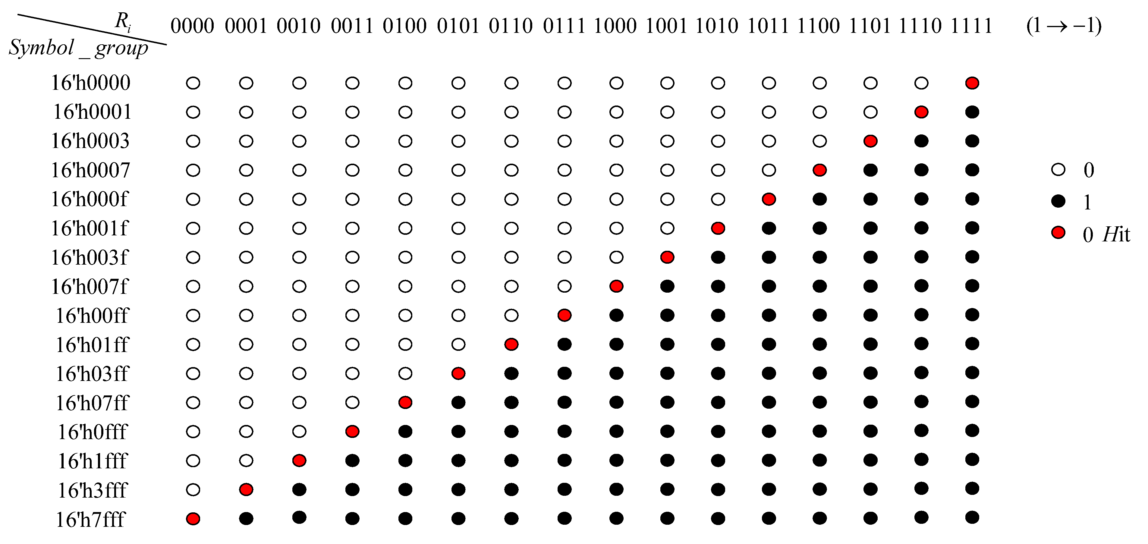
In the prediction of the rotation factor, for each iteration, $\{{\gamma }_i,{\gamma }_{i+1},{\gamma }_{i+2},{\gamma }_{i+3}\}$ can be predicted. In the calculation of the arctangent function, the simplest method is to directly compare the 16 potential branch results of the Y channel and select the one with the absolute value closest to 0. However, if this method is used, a significant amount of area will be consumed, and considerable delay will be introduced in the subsequent hardware circuit design. Therefore, a faster and more area-efficient method is adopted in this paper.

It is known that the value of ${\gamma }_i$ determines whether $(X_i,Y_i)$ requires a clockwise rotation or no rotation to approach the x axis, while $Y_{i+4}$ approaches 0. By examining the highest sign bit of $Y_{i+4}$ in each iteration, we can determine whether the $(X_i,Y_i)$ after rotation crosses the x axis. As shown in Figure 2, the $Symbol$_$group$ represents the highest sign bit of 16 branches of $Y_{i+4}$, and from left to right is the $Y_{i+4}$ corresponding to $\{{\gamma }_i,{\gamma }_{i+1},{\gamma }_{i+2},{\gamma }_{i+3}\}$ from $\{0,0,0,0\}$ to $\{-1,-1,-1,-1\}$ (for the convenience of drawing, −1 is replaced by 1 here). According to Equations (3) and (8) and Table 6, the 16 branches of $Z_{i+4}$ are arranged in ascending order. Therefore, if the left prediction branch has $Y_{i+4}$ as a negative number (the rotation will cross the x axis), then the right prediction branch will have $Y_{i+4}$ as a negative number. Thus, we can ascertain that the values in $Symbol$_$group$ will appear in consecutive 0s or consecutive 1s. Based on this principle, in order for $Y_{i+4}$ to approach 0 without crossing the x axis, a successful prediction $\{{\gamma }_i,{\gamma }_{i+1},{\gamma }_{i+2},{\gamma }_{i+3}\}$ must be located at the boundary between 0 and 1 in $Symbol$_$group$, as indicated by the red mark in Figure 2. Subsequently, we can use the predicted rotation factor $\{{\gamma }_i,{\gamma }_{i+1},{\gamma }_{i+2},{\gamma }_{i+3}\}$ to select the corresponding $X_{i+4}$ and $Z_{i+4}$ from Table 5 and Table 6. With this, one cycle of the four-step parallel branch iteration is completed.

3. Hardware Circuit Implementation of a Four-Precision Floating-Point Arctangent Function

3.1. Top-Level Module

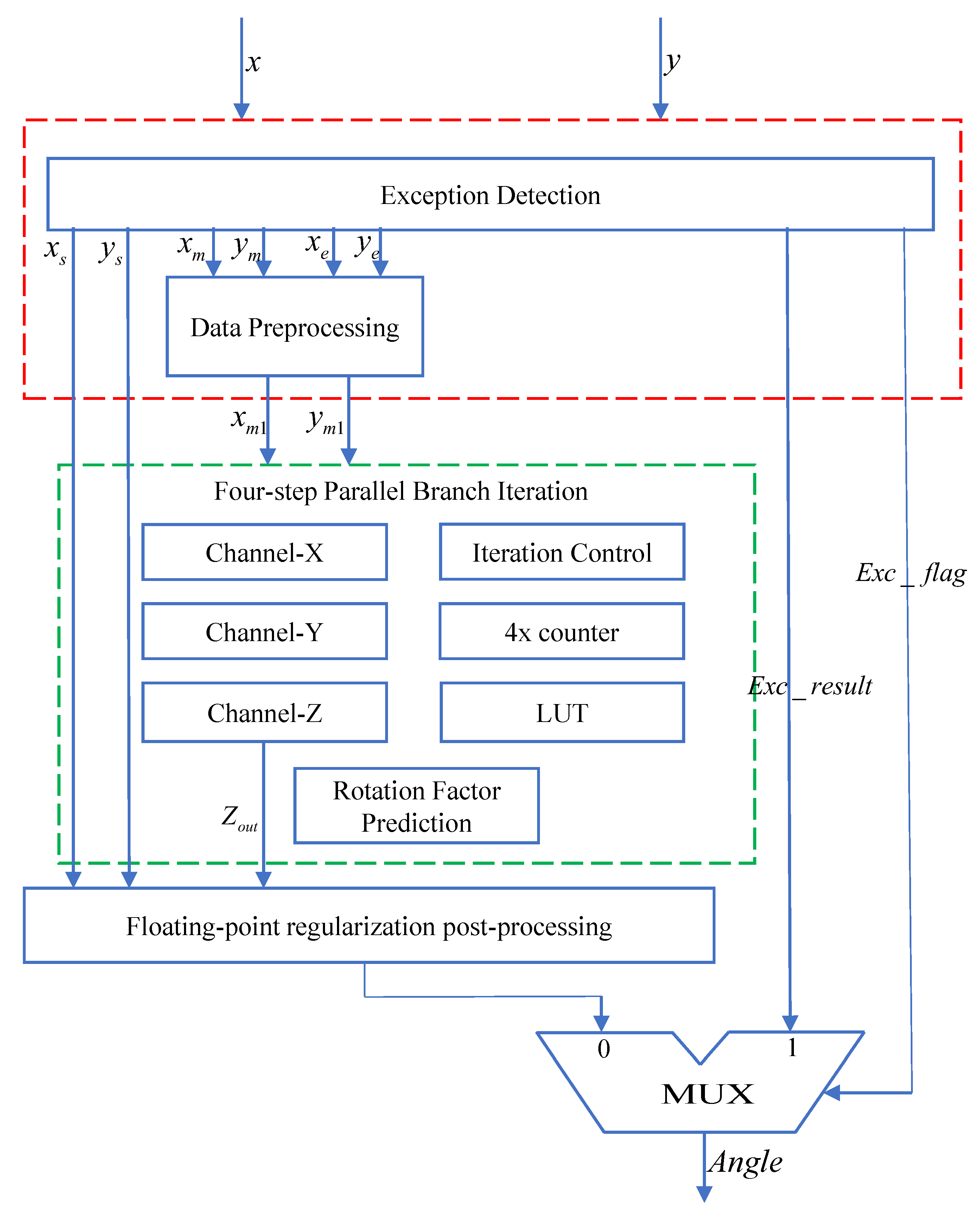
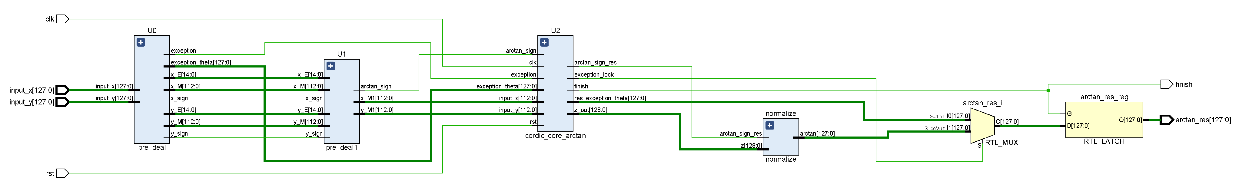
According to the proposed four-precision floating-point arctangent function’s four-step parallel branch iterative CORDIC algorithm, the entire hardware circuit structure mainly consists of three modules: the exception detection and pre-processing module, the four-step parallel branch iteration module, and the floating-point normalization module.

The exception detection and pre-processing module first splits the normalized 128-bit four-precision floating-point input values x and y. Then, based on Table 3 and the arctangent function’s curve, it performs exception detection on the split data. If any exceptions are detected, it outputs the exception flag signal Exc_flag and the result of the exception handling Exc_result. Subsequently, the four-step parallel branch iteration module predicts the rotation factor $\{{\gamma }_i,{\gamma }_{i+1},{\gamma }_{i+2},{\gamma }_{i+3}\}$ and iteratively calculates the three channels $(X,Y,Z)$. After completing the iterations, it processes the output results of the Z channel, converting them from fixed-point to standard four-precision 128-bit floating-point output. Finally, based on the exception flag signal, the module selects the final arctangent result for output.

The hardware structure of the top-level module is illustrated in Figure 3.

3.2. Exception Detection and Pre-Processing Module

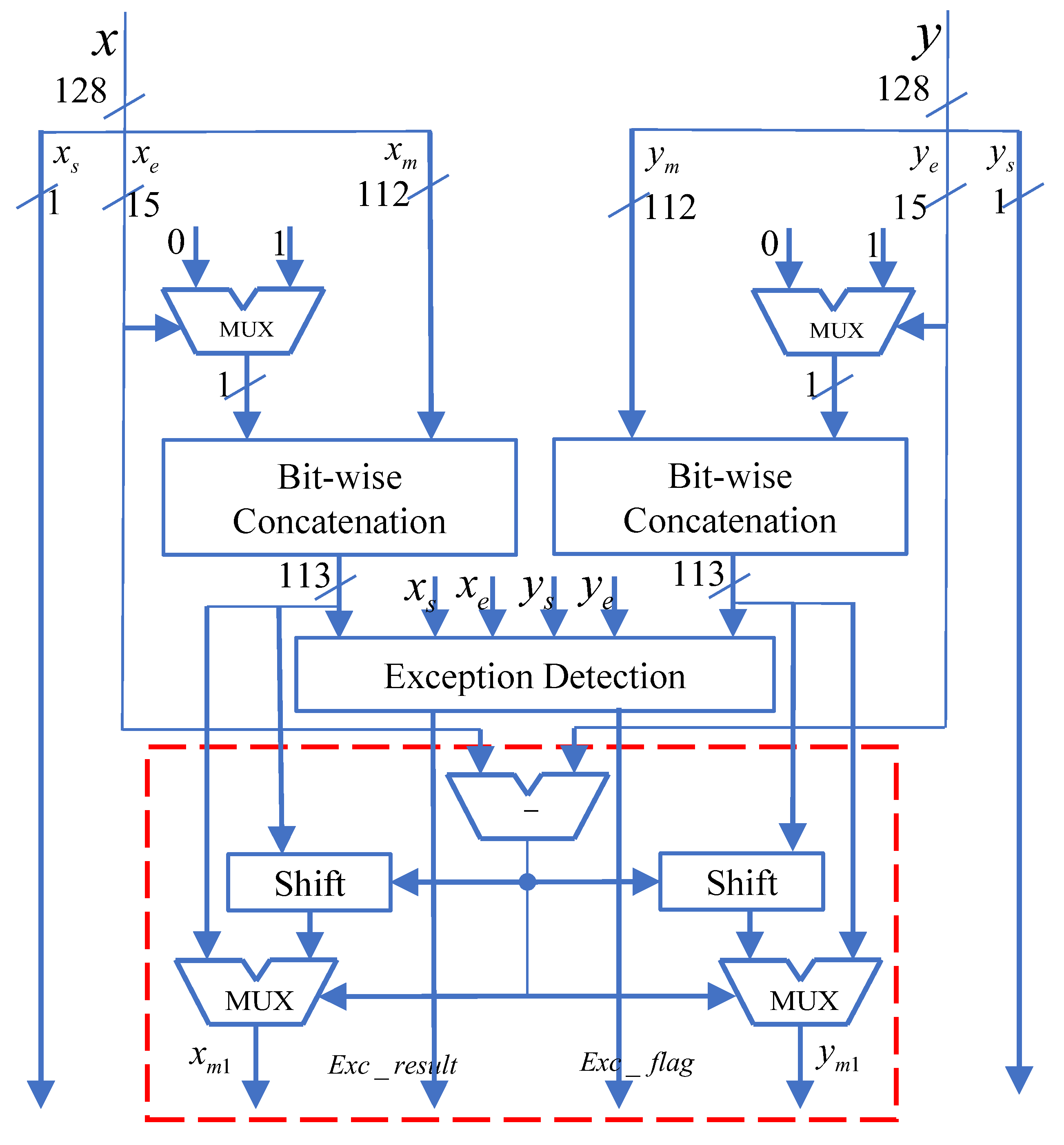
The exception detection and pre-processing module first detects and handles exceptional and special inputs. If the inputs are valid, the module proceeds to pre-process the two input values to ensure they fall within the calculable region of the CORDIC algorithm.

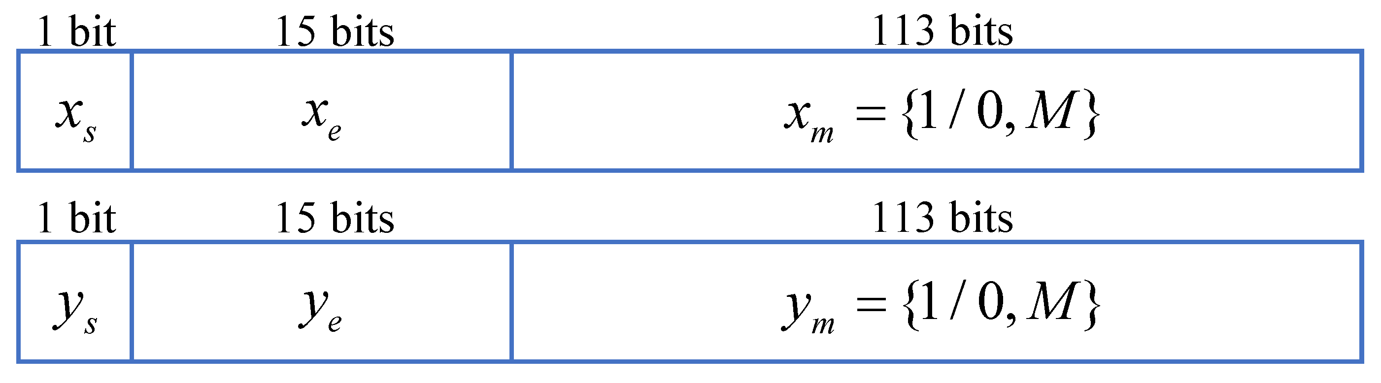
During the process of detecting exceptional and special inputs, the normalized 128-bit floating-point numbers, $xx$ and $yy$, are first split into their respective components: the sign bit, the exponent part, and the fraction part with an added hidden precision bit, as shown in Figure 4. The split data is then subject to exceptional input detection. When exceptional or special inputs are detected, the Exc_flag is set to 1. The possible types of exceptional and special inputs are outlined in

Table 7. Exceptions and special input tables.

${\mathit{x}}_{\mathit{e}}$	${\mathit{x}}_{\mathit{m}}$	${\mathit{x}}_{\mathit{s}}$	${\mathit{y}}_{\mathit{e}}$	${\mathit{y}}_{\mathit{m}}$	${\mathit{y}}_{\mathit{s}}$	Exc_Flag	Exc_Result
15’h7fff	$\ne 0$	-	-	-	-	1	NAN
-	-	-	15’h7fff	$\ne 0$	-	1	NAN
15’h7fff	0	-	15’h7fff	0	-	1	NAN
-	-	-	0	0	-	1	0
0	0	-	-	-	0	1	$\pi /2$
0	0	-	-	-	1	1	$-\pi /2$

.

In the data pre-processing module, in order to enhance the computational precision, both $x_m$ and $y_m$ are extended by 15 bits. Simultaneously, for the computation of the arctangent function, in this design, all input vectors are transformed into the first quadrant, and $x_s$ and $y_s$ are used as quadrant identifiers. Additionally, based on the magnitude of $x_e$ and $y_e$, the following processing is performed to convert the two floating-point numbers into fixed-point numbers without altering their proportional relationship, facilitating subsequent iterative calculations.

(1) When $y_e>x_e$ is true, $x_m$ is right-shifted by $(y_e-x_e)$ bits to obtain $x_{m1}$, and $y_m$ is assigned to $y_{m1}$.

(2) When $y_e<x_e$ is true, $y_m$ is right-shifted by $(x_e-y_e)$ bits to obtain $y_{m1}$, and $x_m$ is assigned to $x_{m1}$.

Here, if $y_e-x_e>128$ is true, then during the shift operation on $x_m$, it will exceed 128 bits, resulting in $x_m$ becoming 0 after the shift. At this point, $arctan(y/x)$’s value approximates $\pm pi/2$, and based on the value of $y_s$, Exc_result is set to $pi/2$ or $-pi/2$. Similarly, if $x_e-y_e>128$ is true, then during the shift operation on $y_m$, it will exceed 128 bits, causing $y_m$ to become 0. As a result, the iterative process of this arithmetic component will not execute, and Exc_result is set to 0.

The circuit structure of the exception detection and pre-processing module is illustrated in Figure 5.

3.3. Four-Step Parallel Branch Iteration Module

The four-step parallel branch iteration module is the core component of the floating-point arctangent function computation unit, which implements the aforementioned four-precision floating-point arctangent function using the four-step parallel branch iterative CORDIC algorithm. This algorithm prioritizes speed over area, employing a single-level loop structure. Its input signals originate from $x_{m1}$ and $y_{m1}$ of the exception detection and pre-processing unit. Through multiple iterations, the module performs parallel computations for the three channels $(X,Y,Z)$ and outputs the arctangent result. Finally, this result, combined with the sign bit preserved by the exception detection and pre-processing unit, is forwarded to the floating-point regularization post-processing module to obtain the final angle value.

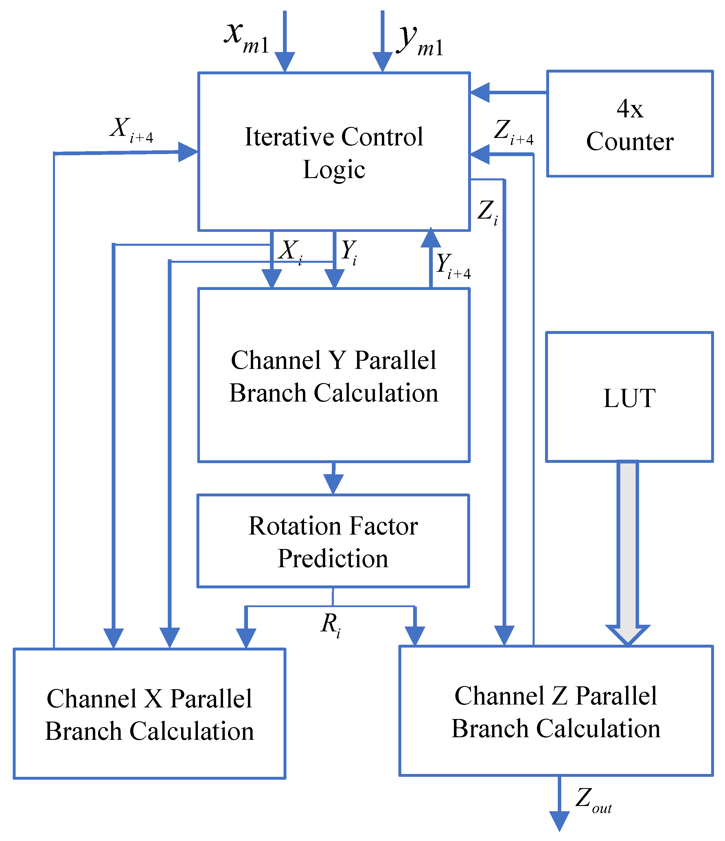
The hardware structure of the four-step parallel branch iteration module is illustrated in Figure 6. It includes a counter, iteration control logic, Y-channel parallel branch computation module, X-channel parallel branch computation module, Z-channel parallel branch computation module, lookup table (LUT), and rotation factor prediction module. In each iteration, the Y-channel first performs parallel computations for 16 predicted branches. Then, the rotation factor prediction module selects the branch $Y_{i+4}$ in the Y-channel that is closest to zero and does not cross the x-axis, obtaining the corresponding value $R_i$ = $\{{\gamma }_i,{\gamma }_{i+1},{\gamma }_{i+2},{\gamma }_{i+3}\}$. Based on $R_i$, the module selects the corresponding branch results $X_{i+4}$ and $Z_{i+4}$ from the X-channel and Z-channel.

3.3.1. Calculation of 16 Branches for X and Y Channels

Through Table 4 and Table 5, it can be observed that among the 16 predicted branches in the Y-channel and X-channel, there are numerous multiplication terms involving the same constant coefficients. To address this issue of multiple-constant multiplication (MCM), a dedicated independent MCM module is designed in this paper. Taking the Y-channel as an example, the split results of the MCM required for its 16 predicted branches are presented in

Table 8. Coefficient split results for multiple-constant multiplication.

First Layer	Split Result	Second Layer	Split Result	Third Layer	Split Result
2	<<1	3	2 + 1	11	8 + 3
4	<<2	5	4 + 1	13	8 + 5
8	<<3	6	2 + 4	22	16 + 6
16	<<4	7	8 − 1	28	16 + 12
32	<<5	9	8 + 1	35	32 + 5
		10	8 + 2
		12	8 + 4
		14	16 − 2
		15	16 − 1

. Initially, the input y undergoes the first-level constant multiplication, where the constants are all powers of 2, readily obtainable through bit shifting. Furthermore, the second-level constants depend on the results from the first level, while the third-level constants necessitate the utilization of the split results from the previous two levels. Thus, by employing appropriate combinations of addition, subtraction, and bit shifting operations, all multiplication terms with their respective constant coefficients can be derived. This method fully utilizes the split results of earlier levels, reducing the number of computations compared to the use of multiple single-constant multipliers. As a result, it addresses the bottleneck issue caused by extensive multiplication calculations, accelerates computation speed, and minimizes area consumption.

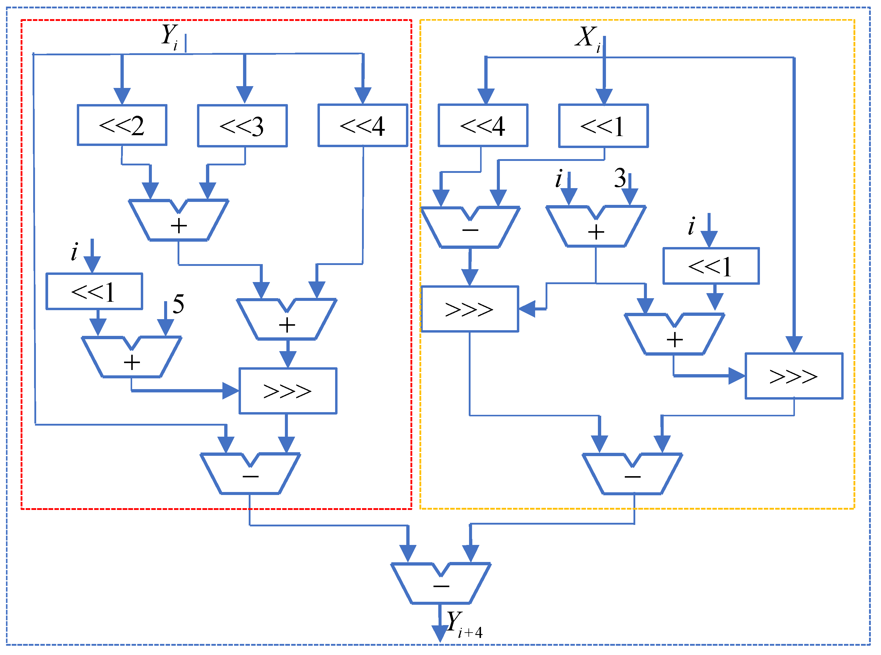
Taking the Y-channel as an example, the specific branch computation structure is provided based on the rules of multiple-constant splitting and the corresponding iterative expressions for $Y_{i+4}$. In Figure 7, the computation process for the 15th branch $Y_{14}$ is illustrated. Initially, $X_i$ and $Y_i$ are fed into the Multiple-Constant Multiplier module. Then, based on the add-4 counter, a shift operation is performed, enabling $X_i$ and $Y_i$ to undergo a left-shift operation before a subsequent right-shift operation. This approach reduces bit loss and effectively enhances precision. To minimize critical path delay, the first two and last two terms of this branch are computed in parallel, followed by a subtraction operation to obtain the final result. The computation principles for the other 15 branches are similar. Similarly, results can be obtained for the 16 branches in the X-channel.

3.3.2. Calculation of 16 Branches for Z-Channel

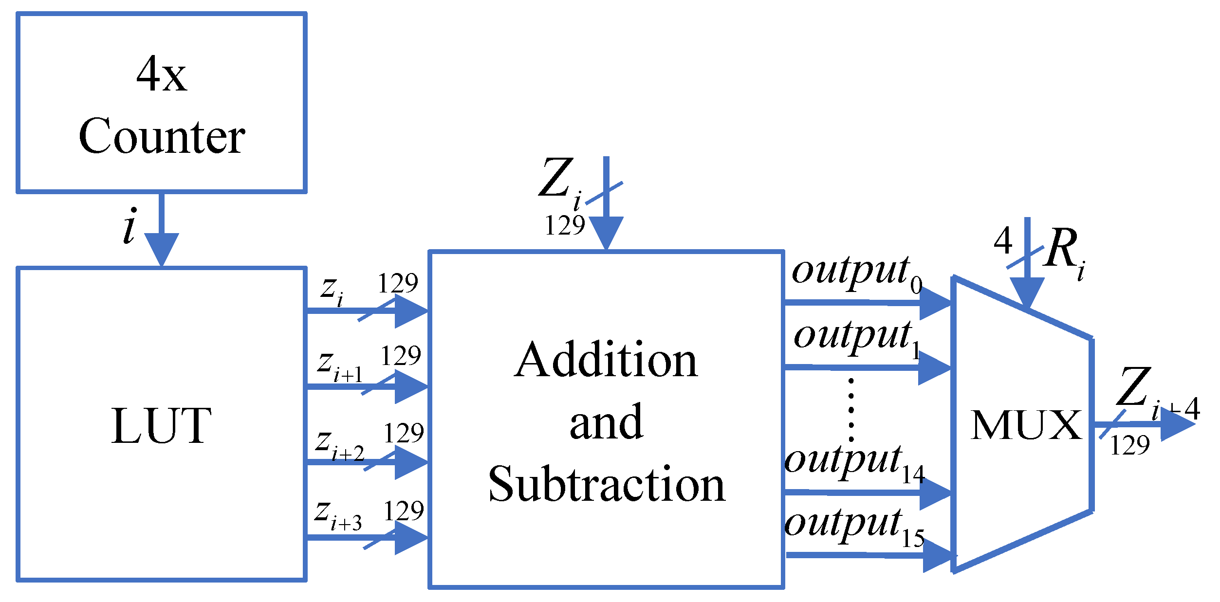
In Table 6, the 16 predicted branches of the Z-channel are obtained through addition and subtraction operations based on precomputed four angles using rotation factors. These four angles are indexed using the output of the add-4 counter and obtained from the lookup table. The lookup table has a bit width of 129 bits, with the highest bit set to 0, preparing for signed addition and subtraction operations in the Z-channel. The precomputed values placed in the lookup table correspond to $arctan\left(1\right)$, $arctan\left(2^{-1}\right)$, $arctan\left(2^{-2}\right)$ and so on. Since all calculations are performed using fixed-point representation, each floating-point arctangent value needs to be converted into fixed-point format before being stored in the lookup table. For a decimal fraction less than 1, its corresponding binary floating-point representation, as shown in Equation (8), can be truncated to the fractional part to obtain the corresponding fixed-point value. Then, by appending a leading 0 to the highest bit, a 129-bit fixed-point value for the lookup table is obtained, as illustrated in Equation (9).

$$Z=0.\stackrel{128bits}{\overbrace{z_0{z}_2{z}_3\cdots z_{126}{z}_{127}}}$$

(9)

$$Z_{Fixed}=\underset{129bits}{\underbrace{0\stackrel{128bits}{\overbrace{z_0{z}_2{z}_3\cdots z_{126}{z}_{127}}}}}$$

(10)

The computation block diagram for the Z-channel is illustrated in Figure 8.

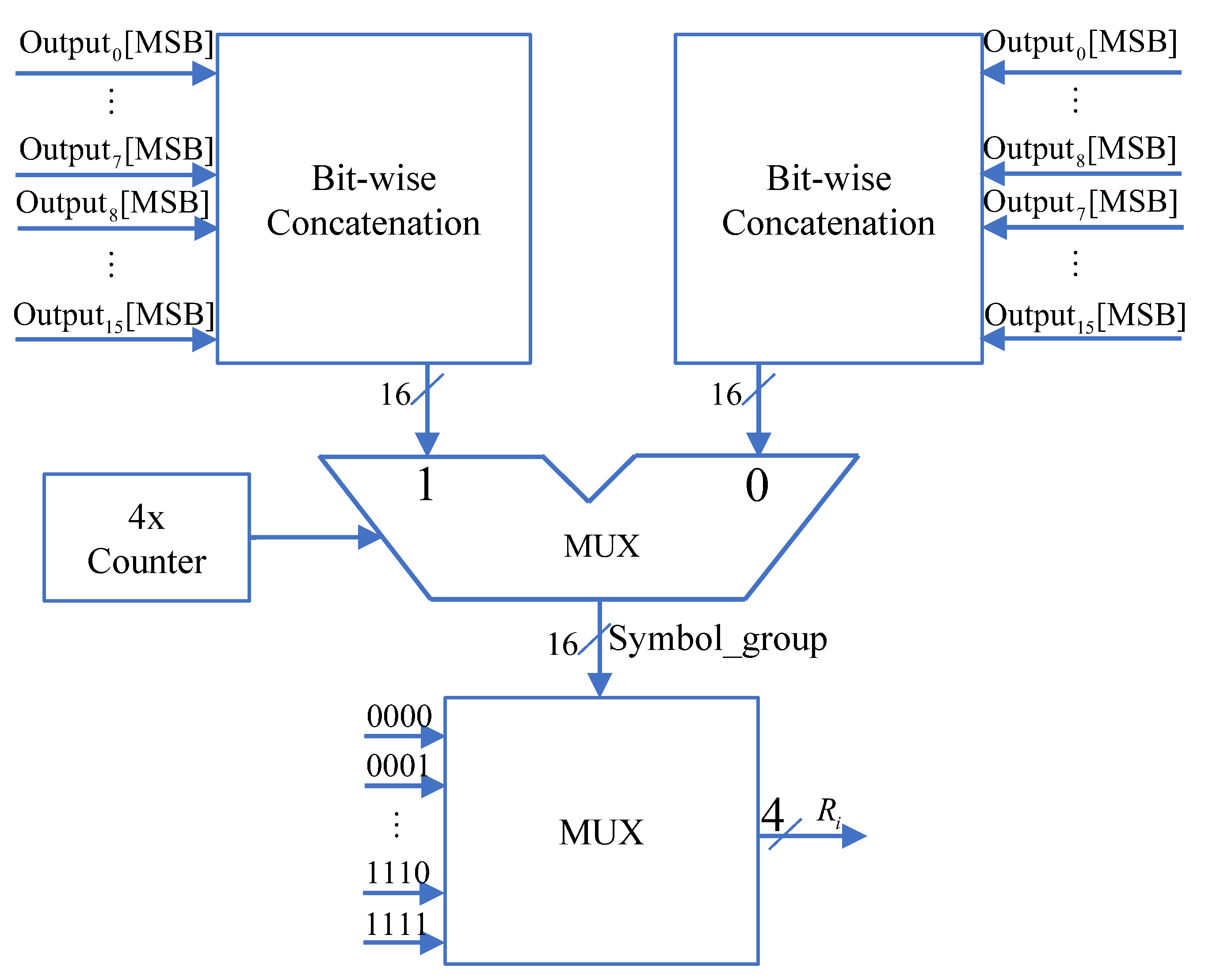
3.3.3. Twiddle Factor Prediction Module

Based on the prediction strategy shown in Figure 2, the highest sign bit of the 16 predicted branches of $Y_{i+4}$, is combined to form a 16-bit Symbol_group selection signal. Subsequently, according to this selection signal, the corresponding rotation factor $R_i$=$\{{\gamma }_i,{\gamma }_{i+1},{\gamma }_{i+2},{\gamma }_{i+3}\}$ is outputted. The relationship between Symbol_group and $R_i$ is presented in

Table 9. The result of the twiddle factor.

Symbol_Group	${\mathit{R}}_{\mathit{i}}$	Symbol_Group	${\mathit{R}}_{\mathit{i}}$
16’h0000	4’b1111	16’h00ff	4’b0111
16’h0001	4’b1110	16’h01ff	4’b0110
16’h0003	4’b1101	16’h03ff	4’b0101
16’h0007	4’b1100	16’h07ff	4’b0100
16’h000f	4’b1011	16’h0fff	4’b0011
16’h001f	4’b1010	16’h1fff	4’b0010
16’h003f	4’b1001	16’h3fff	4’b0001
16’h007f	4’b1000	16’h7fff	4’b0000

. Finally, based on the successfully predicted rotation factor, the corresponding $X_{i+4},Y_{i+4},Z_{i+4}$ is selected as the output result for this iteration.

As $R_i$=$\{{\gamma }_i,{\gamma }_{i+1},{\gamma }_{i+2},{\gamma }_{i+3}\}$ varies from (0, 0, 0, 0) to (−1, −1, −1, −1) incrementally, due to ${\theta }_i>{\theta }_{i+1}>{\theta }_{i+2}>{\theta }_{i+3}$, the values of $Z_0$ to $Z_{15}$, combined with the results of the 16 predicted branches in Table 6, are arranged in ascending order. However, there is a special case where ${\theta }_{i+1}+{\theta }_{i+2}+{\theta }_{i+3}>{\theta }_i$ exists during the first iteration, causing $Z_7>Z_8$. As a result, in the first iteration, the highest sign bits of the two $Y_{i+4}$ corresponding to these $R_i$ should be swapped to ensure that the value of Symbol_group consists of consecutive 0s and consecutive 1s. The hardware structure of the rotation factor prediction module is illustrated in Figure 9.

From Table 8, it can be observed that the maximum constant coefficient in the multiplier is 35. To ensure that the computation process does not result in overflow errors, 6 additional bits should be reserved in $X_i$ and $Y_i$. Moreover, since the current design employs signed arithmetic for addition and subtraction, consideration should be given to a sign bit and an additional carry bit. Thus, before entering the four-step parallel branch iteration module, $X_i$ and $Y_i$ should be padded with 8 bits at the high end to prevent overflow. As the precision of the CORDIC algorithm improves with increasing iteration count, the selection of an appropriate bit width is essential to enhance the precision of the computational results while considering area consumption. Through debugging, this design includes a compensatory bit width of 15 bits appended to the tails of $X_i$ and $Y_i$, resulting in their final bit width being set to 136 bits. Since $Z_i$ involves only addition operations, the lookup table can be set to 128 bits, and adding a carry bit leads to $Z_i$ being set to 129 bits. Thus, each computation requires (113 + 15)/4 = 32 iterations, where 113 represents the fraction bit width and 15 is the compensatory precision. After the completion of 32 iterations, the iterative process concludes, and the output value of Z-channel represents the result of the fixed-point arctangent angle.

3.4. Floating-Point Regularization Post-Processing Module

The floating-point normalization module aims to convert the computed results into floating-point numbers that comply with the IEEE-754 standard. It receives the sign bit from the exception detection and pre-processing module and the 129-bit fixed-point arctangent result from Z-channel after iteration. Through floating-point normalization processing, it eventually outputs a 128-bit floating-point number.

Before performing floating-point normalization, it is necessary to detect leading zeros in the fixed-point arctangent angle value. The conventional approach for leading zero detection involves sequential logic, counting from the highest bit until the first non-zero position is found. However, implementing this structure generally results in significant area and power consumption and is not suitable for this application, especially when there are a large number of leading zeros, requiring multiple detections and significantly slowing down the computation speed. Reference [29] proposes a leading zero detection algorithm based on tree coding, which is efficient for smaller bit widths with fewer encoding and merging operations. However, in this design, the operand is 129 bits long, and applying the tree coding method for leading zero detection would inevitably lead to a long detection chain and considerable gate-level delay.

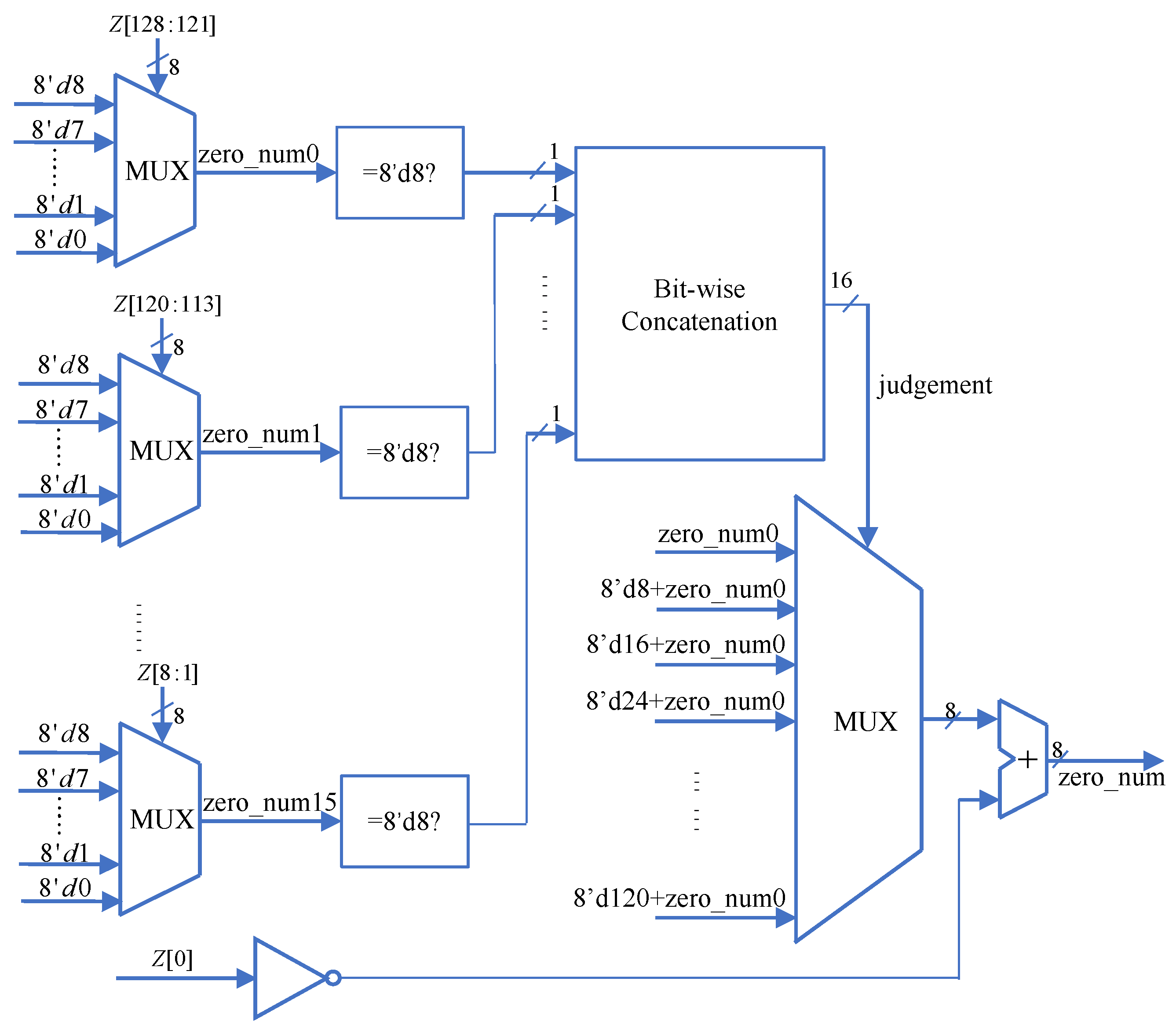
Therefore, in this design, the tree coding method was not chosen, and instead, a multi-way selector was employed to implement the leading zero detection circuit. The multi-way selector is already optimized and readily available in the technology library, offering a smaller delay compared to the tree coding method and a simpler implementation. The 129-bit leading zero detection module in this design consists of two layers of multi-way selectors, and its hardware structure is shown in Figure 10.

First, the 129-bit data to be detected is divided into groups of 8 bits each, forming leading zero detection subunits called lzd_unit. Each subunit takes 8 bits of the data as the selection signal and outputs the number of leading zeros, zero_num, for those 8 bits. Due to the presence of special positions for leading zeros, many terms in the multi-way selector can be combined, significantly reducing the delay. The 129-bit data is divided into 16 groups of 8-bit arrays, with the lowest bit as a separate unit, forming 16 lzd_units and obtaining 16 sets of leading zero counts. Each of these 16 zero_num values is then compared to 8’d8 to check for equality, and the comparison results are concatenated to form a 16-bit determination signal which is called judgment. Finally, judgment is used as the control signal for the multi-way selector to make a selection from the 16 results, ultimately outputting the number of leading zeros for the high 128 bits of the input data. The lowest bit data is combined with the output to obtain the number of leading zeros for the entire 129-bit input data. Since judgment consists of multiple leading ones and the remaining data, it is equivalent to performing leading one detection using the multi-way selector, allowing for further term merging in the selector. The hierarchical connection of the two-layer multi-way selector enables the leading zero detection function to be achieved with minimal delay cost.

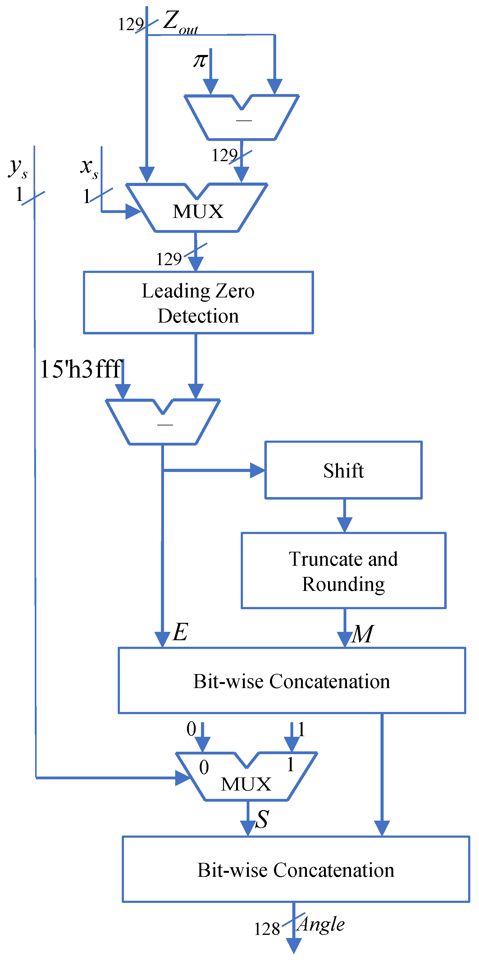
The format of the fixed-point arctangent values is shown in Figure 11, and their corresponding real rad range is between 0 and 2. To convert them into IEEE-754 standard floating-point numbers, the exponent part is determined as (16,383-zero_num) based on the number of leading zeros. Simultaneously, the data is left-shifted by zero_num bits, and the 112 bits following the hidden precision bit 1 are extracted as the mantissa. Finally, combined with the sign bit output from the exception detection and pre-processing module, they form a 128-bit standard floating-point value, resulting in the arctangent angle range of $[-\pi ,\pi ]$. The hardware structure of the floating-point regularization post-processing module is illustrated in Figure 12.

4. Results and Analysis

4.1. Circuit Simulation and Error Comparison

To ensure the accuracy and reliability of the design, we employed the method of random testing and conducted extensive data testing and comparison. Since this design is based on 128-bit floating-point with a maximum precision of 113 bits, the C environment could no longer accommodate quadruple precision. Therefore, we utilized the “bigfloat” package in Python, which supports quadruple precision as well as custom precision. This package allows us to calculate results with the specified precision for input data, making it suitable for conducting tests and comparisons on this module. The data set was generated using a Python script. As Python itself cannot produce standard normalized floating-point numbers, we followed these steps: first, randomly generate 1 bit for the sign, 15 bits for the exponent, and 112 bits for the mantissa. Then, combine these random values to form a standard 128-bit floating-point number and convert it into its corresponding real value. Using the “bigfloat” package, we calculated the arctangent function for the real value and converted the result back into a 128-bit standard floating-point format, saving it as the ideal calculation result. Next, we used the randomly generated standard 128-bit floating-point numbers as the test data set, inputting them into the completed hardware circuit and conducting logic function simulation verification in the modelsim simulation platform. This allowed us to obtain the actual calculation results. Subsequently, we compared the ideal calculation results with the actual calculation results to analyze the discrepancies between them.

From the ideal calculation results and the actual calculation results, we randomly selected 100 sets of data to plot the error scatter diagram, as shown in Figure 13. It can be observed that among the randomly selected 100 sets of test data, the majority of the ideal calculation results have an error smaller than $8.43\times {10}^{-35}$ rad compared to the actual calculation results, with the maximum error not exceeding $2.0\times {10}^{-34}$. Partial ideal calculation results and corresponding actual calculation results are presented in

Table 10. Some simulation and theoretical data.

Input_x	Input_y	Circuit Simulation Result	Python Results
4003136c6f31da68 f9b59fde37a9987c	4003bc40f9d0f2bd ab3d776756ad81bc	3fff040cfa4c18a99 d4a224eda6478f6	3fff040cfa4c18a99 d4a224eda6478f6
4000557faa9d41bd c364e616606e6a7b	40000d64aa536216 7ba90edae51ed46d	3ffe55f81f8ea3463 92516ba70bd7374	3ffe55f81f8ea3463 92516ba70bd7375
4004e265eca703a0 2c54201a3e85d11b	4006426a847f751c ee6b57f49e471c9d	3fff367df31da86b6 16a89fd5d92a646	3fff367df31da86b6 16a89fd5d92a646
40046675def5fa53 5860cc95991d7b4d	3fffc0c4e2b6e40db 73621e047d71840	3ffa4054f9ceaa797 9c88445dc3c9427	3ffa4054f9ceaa797 9c88445dc3c9428
3fff079c82007a74 952bf87b08baaeb4	4000dabae2856163 02494d63af9ee753	3fff4ccb1bbf5bea7 442ca60fc17e706	3fff4ccb1bbf5bea7 442ca60fc17e707
400392583ecb3e6d 21d3e8b18c9966d3	3fffc749be7eb391 3f37f183e0b3976a	3ffb21346986115c 69d4b44dfb408a75	3ffb21346986115c 69d4b44dfb408a7b

.

The testing waveform of the completed system, as depicted in Figure 14, demonstrates that after 32 cycles, a 128-bit floating-point arctangent value satisfying the precision requirement can be obtained.

4.2. Hardware-Implemented Performance

4.2.1. Result Analysis of ASIC Circuit Synthesis

To validate and analyze the completed hardware circuit of the four-precision floating-point arctangent function, logic synthesis was performed on the arctangent function floating-point arithmetic unit using Design Compiler under the TSMC 65 nm process. Power analysis was conducted at a clock frequency of 500 MHz. The arithmetic unit was designed to achieve high precision and low latency by sacrificing power and area.

Table 11. Synthesis results of the circuit.

Process	Area	Power	Iterations
TSMC 65 nm	0.6317 mm${}^2$	40.6483 mW	32

presents the results obtained after synthesis.

Table 12. Iterations for different CORDIC algorithms.

CORDIC Algorithm	Iterations
Traditional CORDIC [8]	113
Radix-4 CORDIC [15]	57
Dual-step branch CORDIC [21]	58
Low-latency hybrid CORDIC [27]	44
This paper	32

presents a comparison of the iteration counts between the four-step parallel branch iterative CORDIC algorithm and other similar low-latency CORDIC algorithms to achieve n-bit precision. The traditional CORDIC algorithm requires n iterations to achieve n-bit precision, while the high-performance radix-4 CORDIC algorithm requires n/2 iterations. The dual-step branch CORDIC algorithm requires (n + 3)/2 iterations, and the low-latency hybrid CORDIC algorithm requires (3n/8) + 1 iterations. With a precision requirement of 113 bits, the results in the table show that the proposed algorithm in this design requires the fewest iterations and achieves the shortest computation period.

4.2.2. Implementation on FPGA

Since the floating-point arctangent function is often used in data signal processing and other fields, it usually needs to be implemented on the FPGA. Therefore, this paper synthesizes and implements the designed hardware circuit on the FPGA, and compares it with the performance of similar computing architectures. The FPGA model we use here is the XC7A100T of the Xilinx Artix-7 series. The circuit diagram of the designed 128-bit floating-point arctangent function upon completion is depicted in Figure 15. Simultaneously, similar algorithms were implemented under the TSMC 65 nm process, and a comparison of hardware circuit costs was conducted.

Table 13. Comparison of hardware cost and performance.

CORDIC	Area on TSMC 65 nm ($\mathbf{m}{\mathbf{m}}^2$)	LUTs Utilized in FPGA	Number of Cycles	Number of Operands	Target Precision (bits)	Error (rad)
Paper [30]	0.0975	5150	22	32	23	$1.9\times {10}^{-6}$
Paper [31]	0.3356	20443	55	64	53	$6\times {10}^{-16}$
This paper	0.6317	37697	32	128	113	$2\times {10}^{-34}$

shows the performance comparison results of the arithmetic unit designed in this paper and other studies.

In Table 13, it can be observed that compared to [30], the proposed arctangent computation unit in this paper has only increased its execution cycles by 10 cycles and consumed 6.3 times more resources. Although there is a slight performance loss in terms of resource consumption and execution efficiency, its computation accuracy has significantly improved, reducing the error by a factor of ${10}^{28}$. Compared to [31], the proposed computation unit in this paper has increased resource consumption by less than 1 time, but it has reduced execution efficiency by 23 cycles. At the same time, the computation accuracy has greatly improved, reducing the error by a factor of ${10}^{18}$. The results indicate that the design strategy of the 128-bit floating-point arctangent computation unit in this paper, which trades area for speed and precision, is highly meaningful and results in significant improvements in computation accuracy and efficiency.

5. Conclusions

In this paper, the traditional CORDIC algorithm is analyzed, considering the issue of low computational efficiency caused by multiple iterations, and an improved four-step parallel branch iterative CORDIC algorithm is proposed, which reduces the computation period by a factor of 4 through parallel prediction of rotation factors, enabling the completion of a 128-bit floating-point arctangent calculation in just 32 cycles. Subsequently, the improved algorithm is implemented and simulated using verilog for hardware circuit implementation, and the results are compared with the “bigfloat” arithmetic library in Python. The result shows that the maximum error does not exceed $2\times {10}^{-34}$ rad, indicating extremely high computational accuracy. Finally, the designed arithmetic unit is subjected to logic synthesis under the TSMC 65 nm process, resulting in a hardware area of approximately 0.6317 mm${}^2$ and power consumption of about 40.6483 mW at a working frequency of 500 MHz. Additionally, the arithmetic unit is also synthesized and implemented on Xilinx FPGA.

Therefore, the designed low-latency four-precision floating-point arctangent algorithm in this paper significantly enhances both the computational accuracy and efficiency of the arctangent function, filling the gap in the research field of high-precision arctangent calculations. Moreover, the arctangent arithmetic unit constructed in this paper fills the void in the domain of high-precision floating-point arctangent hardware circuits, providing a new solution for the design of dedicated CORDIC chips. In the future, this work is intended to be expanded on as follows:

• The designed arithmetic unit will be further improved to reduce the complexity and cost of the hardware circuit;
• The improved algorithm will undergo more extensive experimental validation to verify its correctness in practical applications.