Research on Pattern Recognition Method for φ-OTDR System Based on Dendrite Net

Abstract

The phase-sensitive optical time-domain reflectometer (φ-OTDR) is commonly used in various industries such as oil and gas pipelines, power communication networks, safety maintenance, and perimeter security. However, one challenge faced by the φ-OTDR system is low pattern recognition accuracy. To overcome this issue, a Dendrite Net (DD)-based pattern recognition method is proposed to differentiate the vibration signals detected by the φ-OTDR system, and normalize the differential signals with the original signals for feature extraction. These features serve as input for the pattern recognition task. To optimize the DD for the pattern recognition of the feature vectors, the Variable Three-Term Conjugate Gradient (VTTCG) is employed. The experimental results demonstrate the effectiveness of the proposed method. The classification accuracy achieved using this method is 98.6%, which represents a significant improvement compared to other techniques. Specifically, the proposed method outperforms the DD, Support Vector Machine (SVM), and Extreme Learning Machine (ELM) by 7.5%, 8.6%, and 1.5% respectively. The findings of this research paper indicate that the pattern recognition method based on DD and optimized using the VTTCG can greatly enhance the accuracy of the φ-OTDR system. This improvement has important implications for various applications in industries such as pipeline monitoring, power communication networks, safety maintenance, and perimeter security.

1. Introduction

The distributed fiber optic sensing system based on φ-OTDR overcomes the limitations of traditional Bragg grating-based sensors, which can only monitor external information in a point-by-point manner. It eliminates the need for individual sensor fabrication and can detect vibration information along the entire length of the fiber. The φ-OTDR system offers advantages such as high sensitivity [1], high resolution [2], and a simple structure [3]. It has been widely applied in various fields including pipeline monitoring [4,5], power communication networks [6], and perimeter security [7,8]. In recent years, there have been significant improvements in the performance of φ-OTDR, such as increased sensing fiber length [9] and improved spatial resolution [10,11].

In practical application, the accuracy of the φ-OTDR system is often compromised due to external factors and human interference. To improve the accuracy of system pattern recognition, two strategies are commonly used. One is to enhance the hardware structure [12] by combining the φ-OTDR system with a Mach–Zehnder interferometer [13] or Michelson interferometer [14]. Although this solution can effectively improve recognition accuracy, it also increases the complexity of the hardware structure and system cost.

The second approach is to optimize the pattern recognition method by utilizing machine learning and deep learning techniques [15]. These methods can improve the recognition accuracy of disturbance events. In 2018, Chen et al. utilized the 1D-CNN technique to extract distinctive features from various interference sources based on original events. The accuracy of recognition in monitoring oil pipelines in real-world settings was reported to be 95% [16]. Xu et al. converted various types of vibration signals into spectrograms using spectral subtraction and short-time Fourier transform. These spectrograms were then fed into a CNN with a multi-class support vector machine replacing the soft-max layer to classify different types of vibration signals. The method achieved a recognition accuracy rate of 90% [17]. In 2019, Xin Wang et al. proposed a feature selection method based on the principle of maximum overlap rate. This method selects the most representative feature parameters from a large set and uses the event recognition method of the random forest classifier to identify abnormal events of optical time-domain reflectometry (OTDR). The recognition accuracy rate achieved by this method is 96.58% [18]. In their study on the long-distance φ-OTDR system, Xue Chen et al. extracted both frequency-domain features and time-domain features of the disturbance signal. They utilized an attention-based long short-term memory network as a classifier to accurately identify different types of disturbance signals. The classification accuracy for five typical interference events within the system’s range was found to be 94.3% [19]. In 2020, Yi Shi et al. integrated deep learning and traditional classifiers to extract features from the spatio-temporal data matrix of φ-OTDR. They used a Convolution Neural Network (CNN) to input the matrix and transferred the features to SVM for further classification. However, the accuracy rate of this method is limited to 94.17% when classifying eight types of events due to the constraints of the SVM algorithm [20]. In the same year, Saleh A. Abufana et al. employed the Variational Mode Decomposition (VMD) algorithm to extract high-order statistical features from events and applied a Linear Support Vector Machine (LSVM) to identify disturbance signals at varying signal-to-noise ratio (SNR) levels. However, their classification accuracy was less than 80% [21]. Zhandong Wang et al. utilized the Empirical Mode Decomposition (EMD) method to extract 11 feature vectors from the perturbation signal. They then employed Extreme Gradient Boosting (XGBoost) to attain an average recognition accuracy of 95.89% for the five patterns [22]. In 2022, Wang et al. utilized LSTM to extract timing features from the input signal, while CNN extracted contour and energy features from the time domain curve. They implemented a deep learning network with LSTM and CNN as the main framework, achieving a recognition accuracy of 94.43% for vibration events in the φ-OTDR system [23].

This paper presents a pattern recognition method for a φ-OTDR system using Dendrite Net to address the issue of low accuracy in existing pattern recognition methods. The proposed Dendrite Net [24] uses matrix multiplication and a Hadamard product for its calculations, resulting in low computational complexity. Additionally, the VTTCG [25] is utilized as the optimizer of the DD, with cross entropy serving as the loss function. These techniques have been shown to effectively improve the accuracy and convergence speed of the model. This article utilizes the dataset released by Cao et al. [26] in 2022 to validate the superiority of the VTTCG-DD model. Experiments have demonstrated that this method exhibits better pattern recognition capabilities for the six vibration events (background noise, digging, knocking, watering, shaking, and walking) in the dataset compared to ELM [27] and SVM [28], in terms of both convergence speed and classification accuracy. These results provide evidence of the model’s advantages in terms of generalization and classification accuracy. The contributions of this paper can be summarized as follows:

(1)

In this study, we proposed a novel algorithm for updating the weight matrix in the DD network using the VTTCG algorithm. We conducted experiments to verify the high feasibility and accuracy of the proposed model.

(2)

The proposed algorithm has been demonstrated to outperform other classical pattern recognition methods in terms of recognition accuracy for vibration events in the φ-OTDR system.

The rest of this paper is composed as follows: Section 2 introduces the algorithm principle, including DD and VTTCG; Section 3 is the experiment, consisting of the structure of the φ-OTDR, data preprocessing, the experiment system, and the experimental results; and Section 4 is the conclusion of this paper.

2. Related Work

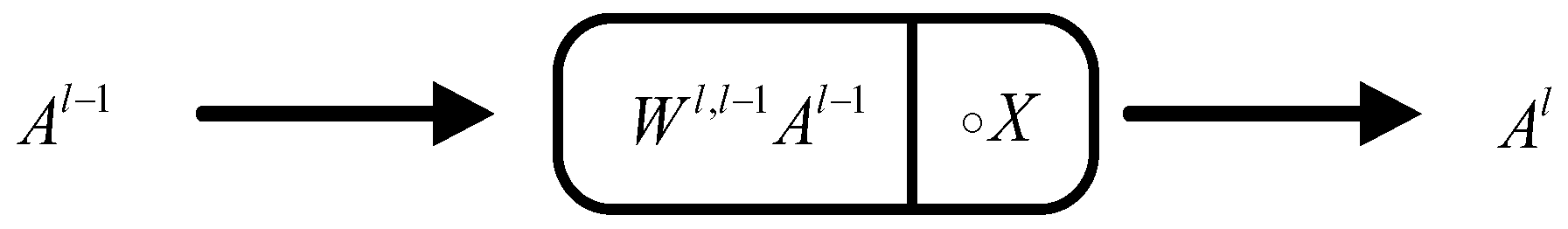
2.1. Introduction of DD

In classification problems, traditional machine learning algorithms divide data based on their characteristics to find a suitable classification curve or surface for solving the problem. However, the resulting model is often a black box model that is difficult to understand and explain. The DD [29] is a white-box algorithm that functions as a logic extractor, enabling it to classify input data without the need to find classification curves or surfaces. It accomplishes this by extracting logical relationship information between input data. Figure 1 displays a basic DD module.

The DD can be expressed as follows:

$${\mathrm{A}}^l=W^{l,l-1}{\mathrm{A}}^{l-1}\circ X$$

(1)

where ${\mathrm{A}}^l$ and ${\mathrm{A}}^{l-1}$ refer to the output and input of the l-th DD module, respectively; $X$ represents the input parameters of DD; $W^{l,l-1}$ denotes the weight matrix from the l-th module to the $\left(l-1\right)\mathrm{th}$ module; and $“\circ ”$ is the Hadamard product operation. The overall structure of the DD is shown in Equation (2):

$$Y=W^{L,L-1}\left[\cdots W^{l,l-1}\left(\cdots W^{21}\left(W^{10}X\circ X\right)\circ X\right)\circ X\cdots \right], L\in N$$

(2)

where $X$ and $Y$ denote the input space and output space, and $L$ is the number of modules. The calculation of DD involves only matrix multiplication and the Hadamard product, making its operation less complex than that of nonlinear functions. DD functions as a logic extractor, extracting the logical relationship information between input data and learning this relationship through training to achieve classification tasks. By using the logical relationship between data to classify, DD avoids the need to look for classification curves or surfaces like traditional machine learning algorithms. This approach makes it easier to interpret and understand the resulting model.

The forward propagation of DD modules and linear modules is as follows:

$$\left\{\begin{array}{l}{\mathrm{A}}^l=W^{l,l-1}{\mathrm{A}}^{l-1}\circ X\\ {\mathrm{A}}^L=W^{L,L-1}{\mathrm{A}}^{L-1}\end{array}\right.$$

(3)

The error back-propagation rules f or the DD and linear modules are as follows:

$${\mathrm{dA}}^L=\widehat{Y}-Y$$

(4)

$$\left\{\begin{array}{l}\mathrm{d}{Z}^L=\mathrm{d}{A}^L\\ \mathrm{d}{Z}^l=\mathrm{d}{A}^l\circ X\end{array}\right.$$

(5)

$${\mathrm{dA}}^{l-1}={\left(W^{l,l-1}\right)}^T\mathrm{d}{Z}^l$$

(6)

The DD performs the adjustment of the weights by gradient descent:

$$\left\{\begin{array}{l}\mathrm{d}{W}^{l,l-1}=\frac{1}{m}\mathrm{d}{Z}^l{\left({\mathrm{A}}^{l-1}\right)}^T\\ W^{l,l-1\left(new\right)}=W^{l,l-1\left(old\right)}-\alpha \mathrm{d}{W}^{l,l-1}\end{array}\right.$$

(7)

In Equation (4), $\widehat{Y}$ and $Y$ are the output of the DD model and the true value. In Equation (7), $m$ refers to the number of samples in a batch during model training. The learning rate, denoted by $\alpha$, controls the gradient descent for weight updates in each iteration. A larger $\alpha$ results in larger step sizes for updates, but may cause the algorithm to fail to converge. Conversely, a smaller $\alpha$ results in smaller step sizes for updates, but may cause the algorithm to converge too slowly.

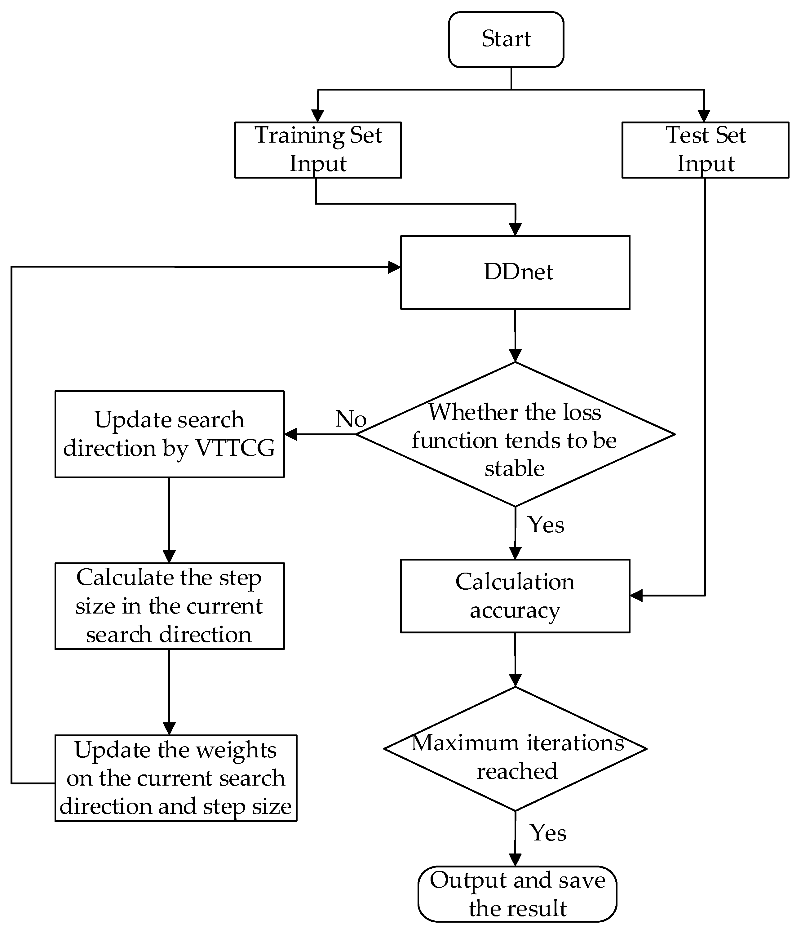
2.2. Variable Three-Term Conjugate Gradient Method for Optimizing DD

The paper proposes a pattern recognition model that uses error backpropagation to adjust the weights of the DD. The loss function chosen in this study is cross-entropy, which is represented by Equation (8):

$$H\left(p,q\right)=-{\displaystyle \sum _{i=1}^n{p}_i\log \left(q_i\right)}$$

(8)

where $p$ is the probability distribution of real labels in the dataset and $q$ is the probability distribution of the classification results of the model. The number of classifications of the model is denoted by ‘n’, which is taken as six since there are six kinds of abnormal events in the data set. The cross entropy is calculated by comparing $p$ and $q$. If they are exactly the same, the cross entropy is 0. The accuracy of the model’s classification can be determined by the value of cross entropy. The smaller the cross entropy, the more accurate the classification of the model.

The VTTCG based on gradient descent is used to continuously reduce the cross-entropy until the global optimal solution is reached during DD model training. The VTTCG is an optimization strategy that utilizes high-order search directions and variable step sizes to find optimal solutions quickly. Compared to other gradient-based optimization algorithms, VTTCG has a faster convergence speed, which can accelerate the neural network’s training process. The VTTCG is a more efficient option for processing large-scale and high-dimensional data compared to high-order optimization algorithms like the traditional Newton method [30] and L-BFGS method [31]. It requires less calculation, making it a better fit for these types of data. The VTTCG adopts a variable step size strategy based on AMSGrad, which effectively avoids the problem of gradient explosion and disappearance [32]. As a result, it is fast, computationally small, and adaptable, making it an ideal choice for optimizing neural network training. Overall, the VTTCG method is an efficient and effective way to improve the efficiency and performance of the model training.

The search direction of the VTTCG is as follows:

$$m_t=-g_t+{\beta }_t^{\mathrm{PRP}}{m}_{t-1}-{\theta }_t{y}_{t-1}$$

(9)

where $g_t$ is the gradient vector of the current iteration point; $y_{t-1}$ is the approximate value of the diagonal elements of the Hessian matrix; and ${\beta }_t^{\mathrm{PRP}}$ and ${\theta }_t$ are algorithm parameters, and the calculation equation is as follows:

$${\beta }_t^{\mathrm{PRP}}=\frac{g_t^T{y}_{t-1}}{{‖g_{t-1}‖}^2}$$

(10)

$${\theta }_t=\frac{g_t^T{m}_{t-1}}{{‖g_{t-1}‖}^2}$$

(11)

where $g_{t-1}$ is the gradient vector of the last iteration point, and $y_{t-1}=g_t-g_{t-1}$; $g_t^T$ is the transposition of the gradient vector $g_t$.

During the model training, the use of variable step size can be beneficial in enabling the network to use a large learning rate for rapid learning in the early stages of training, and gradually decrease the learning rate as the training progresses. This approach can prevent the slow convergence caused by excessively large step sizes, as well as oscillation and other issues, ultimately leading to faster convergence to the optimal solution. The basic form of variable step size in VTTCG is similar to the calculation method of Adam step size [33]. The method of VTTCG variable step size can be broken down into two steps: normalization and stabilization. First, the second moment vector is calculated:

$$a_t=\beta a_{t-1}+\left(1-\beta \right)v_t^2$$

(12)

where $\beta$ is a hyperparameter with a default value of 0.999. $a_t$ is the exponentially weighted average of the gradient square at the t-th iteration, which can be used to estimate the variance of the gradient. $v_t^2$ is the square of the gradient of the loss function to the current parameter. Since the scale of the search direction of the VTTCG is different from that of the Adam, Equation (13) is used to normalize the step size in VTTCG, where $H_t$ is the Hessian matrix of the current iteration point.

$${\alpha }_t=\frac{{\alpha }_t}{\sqrt{g_t^T{H}_t}}$$

(13)

To address the convergence issue that persists despite the normalization when dealing with smaller Batches, the AMSGrad method is utilized to stabilize the step size:

$$\widehat{a}=\max \left({\widehat{a}}_{t-1},a_t\right)$$

(14)

Therefore, the calculation formula of the final variable step size is as follows:

$${\alpha }_t=\frac{\alpha \sqrt{1-{\beta }^t}}{\sqrt{{\widehat{a}}_t}+△}$$

(15)

where $△$ is an extremely small number, avoiding the denominator being 0. Figure 2 shows the classification flow chart of the pattern recognition model for the φ-OTDR system, optimized using the VT-TCG algorithm to improve the DD network.

3. Experiment

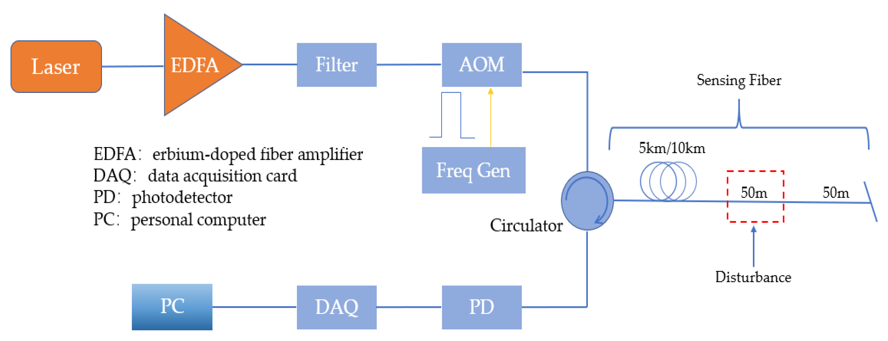
3.1. The Structure of φ-OTDR

The structure of φ-OTDR is illustrated in Figure 3. The light source of this system is an ANKT E15 laser and the pulsed light is amplified continuously by an Erbium-doped fiber amplifier (EDFA). The amplified light is then filtered using a dense wavelength division multiplexer (DWDM) and transmitted through an acousto-optic modulator (AOM) for modulation. The pulsed light is transmitted through a single-mode bare fiber, that is either 5 or 10 km long, via a circulator. To minimize interference from vibrations, the bare fiber is enclosed in a soundproof box. Data are gathered from the first 50 m of the tail 100 m of fiber. The photodetector (PD) receives the Rayleigh backscattered light through the circulator, and the data acquisition card (DAQ) samples the received signal. The digital signal is then stored in a computer for further analysis. The system parameters are as follows: the pulse width is 400 ns and the sampling rate is 10 MSamp/s. When using a 5 km bare fiber, the repetition frequency is 12.5 kHz, and when using a 10 km bare fiber, the repetition frequency is 8 kHz.

Neglecting the influence of noise, the output signal of PD can be simplified as follows:

$$I\left(t\right)=A_{IF}\left(t\right)\cos \left(\Delta \omega t+\phi \left(t\right)\right)$$

(16)

where $A_{IF}\left(t\right)$ represents the signal amplitude information at time $t$, $\Delta \omega$ represents the frequency difference introduced by the AOM, and $\phi \left(t\right)$ represents the signal phase information. In the case of distributed fiber optic sensors, different time $t$ corresponds to different distances on the test fiber. The Hilbert transform is used to demodulate the amplitude and phase of the acquired signal, as shown below:

$$A_{IF}\left(t\right)=\sqrt{I^2\left(t\right)+H{\left[I\left(t\right)\right]}^2}$$

(17)

$$\phi \left(t\right)=\arctan \left(\frac{H\left[I\left(t\right)\right]}{I\left(t\right)}\right)$$

(18)

where $H\left[•\right]$ denotes the Hilbert transform. The amplitude information is obtained by calculating the root mean square of the original signal and the Hilbert transformed signal. The phase information is obtained by solving the arctangent of the ratio between the Hilbert transformed signal and the original signal, followed by unwrapping.

3.2. Data Preprocessing

The φ-OTDR system collected data on six typical events, marked as 0, 1, 2, 3, 4, and 5. These events correspond to background noise, digging, knocking, watering, shaking, and walking. The background noise was collected in the laboratory when no other interference events occurred. The laboratory was located next to a road with passing cars. The digging process involves burying the 5/10 km long sensing fiber tail (50–100 m), which is approximately 10 m in length, in a sandbox that is 15 cm deep. After burying the fiber tail, the excavation is carried out near the sensing fiber. For the knocking event, a 10 m long optical fiber was coiled on an anti-vibration plate, and a hammer was used to hit the plate. The watering event involved evenly watering a 10 m long sensing optical fiber at a height of about 30 cm using a watering can. In the shaking event, the sensing optical fiber was fixed on a fence, and a person standing next to the fence shook different parts of it at a constant rate. For the walking event, a person walked or ran back and forth within about 20 m of the tail of the sensing fiber. To ensure the robustness of the dataset, ten team members collected six vibration events at their tails using two optical fibers (5.1 km and 10.1 km) at different times. The vibration events were collected between distances of 5.0 to 5.05 km and 10.0 to 10.05 km. In the dataset, each sample of each event is composed of 10,000 points in the time domain (0.8 s for 5 km, and 1.25 s for 10 km), and 12 adjacent spatial points (10 m/point) in the space domain. Therefore, the data format for each vibration event was a matrix with 10,000 rows and 12 columns. The number of samples in event data is shown in

Table 1. Sample collection type and quantity.

Even Type	Sample Size	Event Label
Background	3094	0
Digging	2512	1
Knocking	2530	2
Watering	2298	3
Shaking	2728	4
Walking	2450	5

.

To enhance the independence, the stability, and to reduce the serial correlation in the dataset, we perform differentiation on the data. Figure 4 illustrates the spatial-temporal diagram of six distinct event data sets that were collected using a 5 km long sensing fiber. These events include background noise, digging, knocking, watering, shaking, and walking. The Z axis represents dimensionless intensity, and it is evident that the spatial-temporal distribution of various events differs significantly. Background noise is messy in the spatial-temporal matrix. Both single digging and knocking events exhibit distinct peaks, with excavation events displaying a longer duration due to the backflow of sand. Both watering and shaking are continuous events, but shaking occurs with a certain periodicity. Walking events are represented as distinct peaks in each sample based on the individual’s rhythm.

Normalization processing is necessary due to the varying amplitudes of signals. Equation (19) is utilized to normalize the data set.

$$p_m=2\frac{p-p_{\min }}{p_{\max }-p_{\min }}-1$$

(19)

where $p$ refers to the original vector in the dataset. $p_{\min }$ and $p_{\max }$ represent the minimum and maximum values in this vector, respectively. $p_m$ represents the data obtained after normalization, with the value range being $[-1,1]$. To analyze the vibration samples, we extract time-domain features from the normalized data and differential data of each sample’s 1 to 12 channel positions separately. The extracted feature vectors consist of sixteen different factors, such as maximum value, minimum value, peak-to-peak value, mean value, variance, standard deviation, energy, root mean square, rectified mean value, shape factor, margin factor, crest factor, pulse factor, kurtosis factor, and information entropy. The normalized data and the differential data have 12 × 16 = 192 features. These features are concatenated into a vector, which forms the feature vector of a vibration sample.

3.3. Experiment System

To assess the impact of the VTTCG-DD on the classification of abnormal events in the φ-OTDR system, we created a program in Python 3.9 using the PyCharm integrated development environment. We used Pytorch 2.0.0 as the network framework to improve the learning efficiency. In this study, the dataset was divided into a training set and a test set, which accounted for 80% and 20% of the total data set, respectively. The training set consisted of 12,478 sets of sample data, while the test set consisted of 3134 sets of sample data. The VTTCG-DD has a bitch_size of 128 and an initial learning rate of 1e-4. The parameter weight_decay is a type of L2 regularization that modifies the loss function of the model. It encourages the weight parameters of the model to be close to 0, which acts as a penalty mechanism to prevent the model from overfitting the training data. By doing so, it can improve the generalization ability of the model, thus we set it to 5e-4.

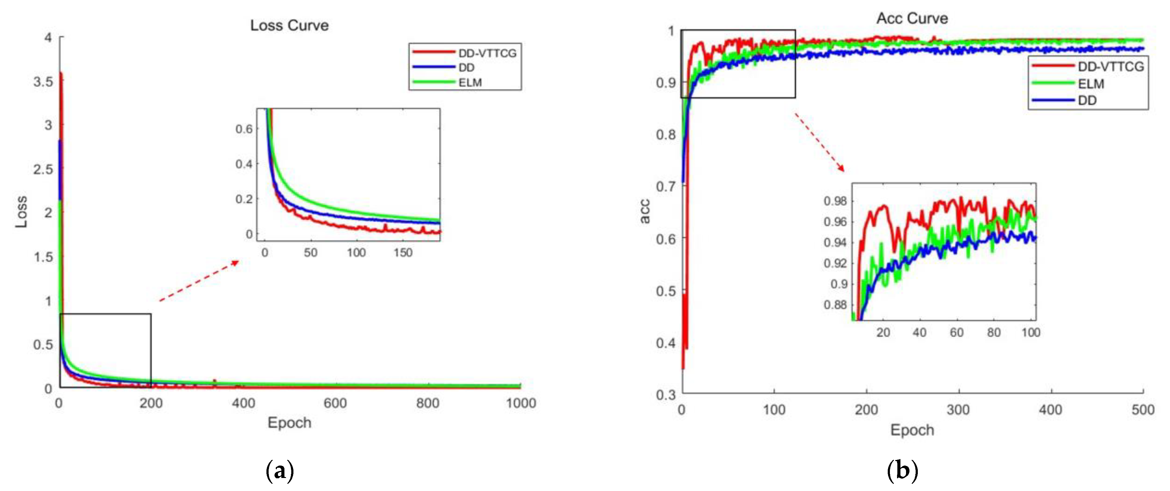
3.4. Experimental Results

In order to evaluate the effectiveness of the proposed network model, this paper compares it with two classic classification algorithms, namely, SVM and ELM, as well as DD, using the φ-OTDR abnormal event dataset. The ELM algorithm is a single-layer feed-forward neural network algorithm. During the training process, the weights and biases from the input layer to the hidden layer are randomly initialized, and then the weights of the output layer are directly calculated. However, this randomness can lead to the unstable performance of the model and potentially result in large generalization errors. The loss function can be seen in Figure 5a. According to Figure 5, the DD network optimized by VTTCG demonstrates faster convergence speed, lower training loss, and higher classification rate compared to the ELM algorithm and the original DD network. The test accuracy curve and loss function curve of the ELM model gradually converge to 97.5% and 0.16 after approximately 400 epochs. Similarly, the test accuracy curve and loss function curve of the original DD network converge to 91.2% and 0.25 after the same 400 epochs. On the other hand, the VTTCG-DD model only requires about 150 epochs for the test accuracy curves and loss function curves to gradually converge to 98.6% and 0.13.The results indicate that the DD optimized by the VTTCG outperforms the original DD network model and ELM model in terms of both training loss and convergence speed on this dataset. Figure 5b displays a comparison of the classification accuracy of the model using the test set. The optimized DD model’s classification accuracy converges at 98.62%, which is approximately 7.42% higher than the original DD. The classification accuracy of the ELM is comparable to that of the optimized DD. However, the DD exhibits a higher convergence speed compared to the ELM.

SVM is a machine learning algorithm primarily utilized for solving regression and pattern recognition problems, especially when dealing with small samples. The algorithm’s main objective is to construct an optimal classification boundary that maximizes the interval between classifications. This is achieved by classifying data using support vectors. After performing feature extraction, the resulting dataset in this paper will generate a feature matrix with a size of 15,612 by 384, consisting of 12,478 training sets and 3134 test sets. Therefore, reducing the dimensionality of the feature matrix can help the SVM achieve optimal pattern recognition results. In this study, the method of principal component analysis (PCA) [34] was utilized to reduce the dimension of the feature matrix. The parameter n_components was set to 0.95 to retain 95% of the information of the feature after dimension reduction. The resulting feature matrix size was 15,612 × 59. SVM and VTTCG-DD models were trained using the training set. Figure 6a demonstrates that the SVM algorithm achieved the highest recognition accuracy of 99.8% for background noise events labeled as 0. It is evident that there are distinct differences between background noise events and the other five disturbance events. However, the model performed poorly in recognizing digging events, with a classification accuracy of only 80.5%. On the other hand, Figure 6b shows that the pattern recognition method utilizing the VTTCG-optimized DD network achieved the highest recognition rate for background noise, knocking, and shaking events, which exhibited significant improvement compared to the SVM model. However, it had the worst recognition results for watering events.

Table 2. Recognition of abnormal events in φ-OTDR based on SVM.

Label	Precison	Recall	F1-Score	Test Set	Misclassified Samples
0	0.99	0.88	0.93	619	1
1	0.80	0.80	0.80	502	98
2	0.90	0.95	0.92	506	49
3	0.80	0.98	0.88	471	93
4	0.99	0.93	0.96	546	6
5	0.87	0.88	0.87	490	66

shows the SVM recognition results of φ-OTDR abnormal events. The table presents Precision, Recall, and F1-score as indicators to measure the classification accuracy of SVM. The results indicate an average accuracy of 90.01%, with misclassified samples mainly concentrated in categories 1 (digging) and 3 (watering).

The accuracy of identifying φ-OTDR abnormal events using the classification algorithm used in this paper was determined by taking the average value after running the experiment 15 times, as presented in

Table 3. Method accuracy comparison.

Optimized DD	Original DD	ELM	SVM
98.6%	91.2%	97.5%	90.0%

.

The results demonstrate that utilizing the VTTCG optimization algorithm to optimize the DD results in a higher classification accuracy compared to the original DD network, thus confirming the algorithm’s superiority. The DD, optimized by the VTTCG algorithm, exhibits slightly higher classification accuracy than the ELM. It also boasts a faster convergence speed compared to the ELM. Moreover, it outperforms the traditional machine learning method SVM by 8.6% in terms of classification accuracy. Therefore, the optimized DD is a superior choice for pattern recognition in the φ-OTDR system.

4. Conclusions

This paper proposes a pattern recognition method based on the DD network model to address the problem of low pattern recognition accuracy in a φ-OTDR distributed optical fiber vibration sensing system. The method involves extracting features from the original data and the difference data, and connecting them into a feature vector. This approach allows for the retaining of the trend and periodicity of the original data, while also capturing small changes in the data based on the difference data. As a result, the accuracy of the model is improved. The extracted features are then fed into the DD network model, which is optimized with VTTCG.

To evaluate the performance of our algorithm, we compared two classic classification algorithms—support vector machine and extreme learning machine—with the DD network on the φ-OTDR abnormal event dataset. The experimental results demonstrate that our proposed recognition method, using the VTTCG-optimized DD network model, achieves a high classification accuracy of 98.6%. We tested six typical perturbation events, including background noise, digging, knocking, watering, shaking, and walking. The original DD network, SVM, and ELM accurately identified all of these events. Therefore, the pattern recognition method proposed in this paper, which utilizes the DD network optimized by VTTCG, can effectively distinguish different types of event signals with a high accuracy rate. This is significant for enhancing the performance of the distributed optical fiber disturbance sensing system.

References

1. Tu, G.; Yu, B.; Zhen, S.; Qian, K.; Zhang, X. Enhancement of signal identification and extraction in a Φ-OTDR vibration sensor. IEEE Photonics J. 2017, 9, 1–10. [Google Scholar] [CrossRef]
2. Zhu, F.; Zhang, Y.; Xia, L.; Wu, X.; Zhang, X. Improved Φ-OTDR sensing system for high-precision dynamic strain measurement based on ultra-weak fiber Bragg grating array. J. Light. Technol. 2015, 33, 4775–4780. [Google Scholar]
3. Mei, X.; Pang, F.; Liu, H.; Yu, G.; Shao, Y.; Qian, T.; Mou, C.; Lv, L.; Wang, T. Fast coarse-fine locating method for φ-OTDR. Opt. Express 2018, 26, 2659–2667. [Google Scholar] [CrossRef] [PubMed]
4. Wu, H.; Liu, X.; Xiao, Y.; Rao, Y. A dynamic time sequence recognition and knowledge mining method based on the hidden Markov models (HMMs) for pipeline safety monitoring with Φ-OTDR. J. Light. Technol. 2019, 37, 4991–5000. [Google Scholar] [CrossRef]
5. Hu, Y.; Meng, Z.; Ai, X.; Li, H.; Hu, Y.; Zhao, H. Hybrid Feature extraction of pipeline microstates based on Φ-OTDR sensing system. J. Control Sci. Eng. 2019, 2019, 6087582. [Google Scholar] [CrossRef]
6. Ding, Z.-W.; Zhang, X.-P.; Zou, N.-M.; Xiong, F.; Song, J.-Y.; Fang, X.; Wang, F.; Zhang, Y.-X. Phi-OTDR based on-line monitoring of overhead power transmission line. J. Light. Technol. 2021, 39, 5163–5169. [Google Scholar] [CrossRef]
7. Juarez, J.C.; Taylor, H.F. Field test of a distributed fiber-optic intrusion sensor system for long perimeters. Appl. Opt. 2007, 46, 1968–1971. [Google Scholar] [CrossRef] [PubMed]
8. Zhang, X.; Sun, Z.; Shan, Y.; Li, Y.; Wang, F.; Zeng, J.; Zhang, Y. A high performance distributed optical fiber sensor based on Φ-OTDR for dynamic strain measurement. IEEE Photonics J. 2017, 9, 1–12. [Google Scholar] [CrossRef]
9. Martins, H.F.; Martin-Lopez, S.; Corredera, P.; Ania-Castañon, J.D.; Frazão, O.; Gonzalez-Herraez, M. Distributed vibration sensing over 125 km with enhanced SNR using phi-OTDR over a URFL cavity. J. Light. Technol. 2015, 33, 2628–2632. [Google Scholar] [CrossRef]
10. Marcon, L.; Soto, M.A.; Soriano-Amat, M.; Costa, L.; Martins, H.F.; Palmieri, L.; Gonzalez-Herraez, M. Boosting the spatial resolution in chirped pulse ϕ-OTDR using sub-band processing. In Proceedings of the Seventh European Workshop on Optical Fibre Sensors, Limassol, Cyprus, 1–4 October 2019; pp. 295–298. [Google Scholar]
11. Yan, Q.; Tian, M.; Li, X.; Yang, Q.; Xu, Y. Coherent φ-OTDR based on polarization-diversity integrated coherent receiver and heterodyne detection. In Proceedings of the 2017 25th Optical Fiber Sensors Conference (OFS), Jeju, Republic of Korea, 24–28 April 2017; pp. 1–4. [Google Scholar]
12. Juarez, J.C.; Maier, E.W.; Choi, K.N.; Taylor, H.F. Distributed fiber-optic intrusion sensor system. J. Light. Technol. 2005, 23, 2081–2087. [Google Scholar] [CrossRef]
13. Liang, S.; Sheng, X.; Lou, S.; Feng, Y.; Zhang, K. Combination of phase-sensitive OTDR and michelson interferometer for nuisance alarm rate reducing and event identification. IEEE Photonics J. 2016, 8, 1–12. [Google Scholar] [CrossRef]
14. He, H.; Shao, L.-Y.; Luo, B.; Li, Z.; Zou, X.; Zhang, Z.; Pan, W.; Yan, L. Multiple vibrations measurement using phase-sensitive OTDR merged with Mach-Zehnder interferometer based on frequency division multiplexing. Opt. Express 2016, 24, 4842–4855. [Google Scholar] [CrossRef]
15. Kandamali, D.F.; Cao, X.; Tian, M.; Jin, Z.; Dong, H.; Yu, K. Machine learning methods for identification and classification of events in ϕ-OTDR systems: A review. Appl. Opt. 2022, 61, 2975–2997. [Google Scholar] [CrossRef] [PubMed]
16. Chen, J.; Wu, H.; Liu, X.; Xiao, Y.; Wang, M.; Yang, M.; Rao, Y. A real-time distributed deep learning approach for intelligent event recognition in long distance pipeline monitoring with DOFS. In Proceedings of the 2018 International Conference on Cyber-Enabled Distributed Computing and Knowledge Discovery (CyberC), Zhengzhou, China, 18–20 October 2018; pp. 290–2906. [Google Scholar]
17. Xu, C.; Guan, J.; Bao, M.; Lu, J.; Ye, W. Pattern recognition based on time-frequency analysis and convolutional neural networks for vibrational events in φ-OTDR. Opt. Eng. 2018, 57, 016103. [Google Scholar] [CrossRef]
18. Wang, X.; Liu, Y.; Liang, S.; Zhang, W.; Lou, S. Event identification based on random forest classifier for Φ-OTDR fiber-optic distributed disturbance sensor. Infrared Phys. Technol. 2019, 97, 319–325. [Google Scholar] [CrossRef]
19. Chen, X.; Xu, C. Disturbance pattern recognition based on an ALSTM in a long-distance φ-OTDR sensing system. Microw. Opt. Technol. Lett. 2020, 62, 168–175. [Google Scholar] [CrossRef]
20. Shi, Y.; Wang, Y.; Wang, L.; Zhao, L.; Fan, Z. Multi-event classification for Φ-OTDR distributed optical fiber sensing system using deep learning and support vector machine. Optik 2020, 221, 165373. [Google Scholar] [CrossRef]
21. Abufana, S.A.; Dalveren, Y.; Aghnaiya, A.; Kara, A. Variational mode decomposition-based threat classification for fiber optic distributed acoustic sensing. IEEE Access 2020, 8, 100152–100158. [Google Scholar] [CrossRef]
22. Wang, Z.; Lou, S.; Liang, S.; Sheng, X. Multi-class disturbance events recognition based on EMD and XGBoost in φ-OTDR. IEEE Access 2020, 8, 63551–63558. [Google Scholar] [CrossRef]
23. Wang, M.; Feng, H.; Qi, D.; Du, L.; Sha, Z. φ-OTDR pattern recognition based on CNN-LSTM. Optik 2023, 272, 170380. [Google Scholar] [CrossRef]
24. Liu, G.; Wang, J. Dendrite net: A white-box module for classification, regression, and system identification. IEEE Trans. Cybern. 2021, 52, 13774–13787. [Google Scholar] [CrossRef] [PubMed]
25. Kim, H.; Wang, C.; Byun, H.; Hu, W.; Kim, S.; Jiao, Q.; Lee, T.H. Variable three-term conjugate gradient method for training artificial neural networks. Neural Netw. 2023, 159, 125–136. [Google Scholar] [CrossRef] [PubMed]
26. Cao, X.; Su, Y.; Jin, Z.; Yu, K. An open dataset of φ-OTDR events with two classification models as baselines. Results Opt. 2023, 10, 100372. [Google Scholar] [CrossRef]
27. Zhang, M.; Li, Y.; Chen, J.; Song, Y.; Zhang, J.; Wang, M. Event detection method comparison for distributed acoustic sensors using φ-OTDR. Opt. Fiber Technol. 2019, 52, 101980. [Google Scholar] [CrossRef]
28. Xu, C.; Guan, J.; Bao, M.; Lu, J.; Ye, W. Pattern recognition based on enhanced multifeature parameters for vibration events in φ-OTDR distributed optical fiber sensing system. Microw. Opt. Technol. Lett. 2017, 59, 3134–3141. [Google Scholar] [CrossRef]
29. Liu, G. It may be time to improve the neuron of artificial neural network. TechRxiv Prepr. 2021, 7–21. [Google Scholar] [CrossRef]
30. Mangasarian, O.L. A finite Newton method for classification. Optim. Methods Softw. 2002, 17, 913–929. [Google Scholar] [CrossRef]
31. Berahas, A.S.; Nocedal, J.; Takác, M. A multi-batch L-BFGS method for machine learning. Adv. Neural Inf. Process. Syst. 2016, 29. [Google Scholar] [CrossRef]
32. Tran, P.T. On the convergence proof of amsgrad and a new version. IEEE Access 2019, 7, 61706–61716. [Google Scholar] [CrossRef]
33. Bock, S.; Goppold, J.; Weiß, M. An improvement of the convergence proof of the ADAM-Optimizer. arXiv 2018, arXiv:1804.10587. [Google Scholar]
34. Bhattacharya, S.; Maddikunta, P.K.R.; Kaluri, R.; Singh, S.; Gadekallu, T.R.; Alazab, M.; Tariq, U. A novel PCA-firefly based XGBoost classification model for intrusion detection in networks using GPU. Electronics 2020, 9, 219. [Google Scholar] [CrossRef]
Figure 1. DD Foundation Module.
Electronics 12 03757 g001
Figure 2. Classification flowchart of φ-OTDR system pattern recognition model based on the VTTCG to optimize the DD.
Electronics 12 03757 g002
Figure 3. Structure diagram of φ-OTDR system.
Electronics 12 03757 g003
Figure 4. Spatial-temporal diagram after differentiating of six typical events: (a) background noise; (b) digging; (c) knocking; (d) watering; (e) shaking; and (f) walking.
Electronics 12 03757 g004
Figure 5. Experimental results of the dataset: (a) Model loss function comparison; (b) Model classification accuracy comparison.
Electronics 12 03757 g005
Figure 6. The test set confusion matrix of the two algorithms: (a) The confusion matrix of the SVM algorithm for the test set; (b) The confusion matrix of the VTTCG-DD algorithm for the test set.
Electronics 12 03757 g006