Software Design for Airborne GNSS Air Service Performance Evaluation under Ionospheric Scintillation

Abstract

The performance analysis and evaluation of satellite navigation systems under ionospheric scintillation have been a focal point in the field of modern aviation. With the development and upgrading of satellite navigation systems, the performance indicators and evaluation techniques of these systems also require continuous iteration and optimization. In this study, based on the ionospheric scintillation model and satellite navigation algorithm, we designed a software tool to evaluate the performance of GNSS aviation services under various ionospheric scintillation intensities. The software is implemented in the C/C++ programming language and provides assessment capabilities for different ionospheric scintillation environments and flight phases. By encapsulating the software task modules using technologies such as dynamic link libraries and thread pools, the software can flexibly adjust the ionospheric scintillation intensity and control the flight trajectory. This ensures the strong scalability and reusability of the software. The software supports the performance evaluation of aviation services during all flight phases of global flights and is compatible with GPS, BDS, GALILEO, and GLONASS systems. Through verification of the accuracy, integrity, continuity, and availability of the GNSS system under different flight phases and ionospheric scintillation effects, the effectiveness of the software design has been validated.

1. Introduction

The development of GNSS has established its significance as a core technology in modern aviation over the past few decades. The exceptional reliability and precision offered by GNSS have emerged as crucial factors in ensuring flight safety. Nonetheless, it is important to acknowledge that satellite signals are vulnerable to environmental factors, such as ionospheric and tropospheric anomalies, which serve as the primary sources of error in GNSS for aviation applications [1]. Alterations in the ionospheric environment can induce delay effects and ionospheric scintillation, thereby deteriorating or even impeding the performance of GNSS systems and posing a potential hazard to aviation safety. Existing atmospheric anomaly correction models have proven effective in mitigating the influence of tropospheric and ionospheric delays on GNSS signals at present [2]. However, comprehending the intricate impacts of ionospheric scintillation on GNSS performance necessitates conducting simulations of ionospheric scintillation environments and evaluating GNSS performance within anomalous conditions. These endeavors hold immense value and significance in enhancing GNSS performance and augmenting its precision.

Initially proposed by Professor A.J. Van Dierendonck, the AJ-Stanford ionospheric scintillation model is based on a statistical approach and was subsequently implemented by S. Pullen’s team [3]. Extensive validation and correction of the model were conducted using a substantial volume of measured data, resulting in a high level of prediction accuracy. While the model has achieved remarkable success in GPS applications [4], it does have certain limitations. Specifically, its applicability to ionospheric scintillation in equatorial regions may be limited, as it is primarily suitable for addressing ionospheric scintillation in moderate and high latitudes. In addition to the AJ-Stanford model, T. Humphreys made significant contributions to the field by introducing novel statistical methods and mathematical models, leading to the development of the Cornell model [5,6]. This model has been made open-source, serving as a valuable resource for the simulation of ionospheric scintillation signals. The Cornell model not only serves as an important reference in the field but has also contributed to the advancement of ionospheric scintillation research.

Axel Garcia-Pena and colleagues conducted an analysis of performance variations among airborne systems operating in different frequency bands and under diverse interference environments. Their research led to the development of a performance evaluation method based on link budgets, which offers experimental validation for GNSS performance testing and analysis efforts [7]. The magicIFP platform enables the comparative assessment of actual flight paths and navigation solutions to evaluate the performance of navigation systems across various aircraft models and under different weather condition settings [8]. In addition, the Stanford GPS Laboratory has developed a simulation tool called the MATLAB Algorithm Availability Simulation Tool (MAAST) [9] based on the Service Volume Model (SVM). This tool allows the investigation of service performance evaluation methods by simulating various atmospheric environments and constellation configurations. Furthermore, the Galileo research team has developed an evaluation tool called the GALILEO System Simulation Facility (GSSF) [10], which integrates raw ephemeris data and allows users to evaluate service performance over extended durations by simulating multiple environments.

This paper proposes a software design method that combines ionospheric scintillation environment simulation and GNSS performance evaluation algorithms. The objective is to simulate and evaluate the performance of GNSS aviation services in different ionospheric scintillation conditions utilizing Receiver Independent Exchange Format (RINEX) files [11]. The software is developed for the Windows 10 operating system and implemented using the C/C++ programming language with Visual Studio and the QT platform. It is divided into several functional modules, including a graphical user interface (GUI) module, a data source generation module, an anomaly detection module, and a performance evaluation module [12]. These modules work together to simulate and evaluate the performance of GNSS aviation services. To validate the software’s feasibility, the performance evaluation module supports the evaluation of GNSS data from eight frequency points, including GPS L1/L2, BDS B1/B2a, GALILEO E1/E5b, and GLONASS G1/G2. The evaluation criteria in this study are based on the Requested Navigation Performance (RNP) defined by the International Civil Aviation Organization (ICAO). These criteria encompass parameters such as accuracy, integrity, continuity, and availability [13]. The software enables the comparison and analysis of performance evaluation results for airborne GNSS systems across different flight phases, including scenarios without ionospheric scintillation and those with strong ionospheric scintillation environments. Its GUI interface supports flight plan querying and track monitoring functions. Moreover, data processing techniques such as dynamic link libraries and thread pools are employed to optimize the software’s running speed and smoothness [14].

In Section 2 of the paper, the RINEX file generation scheme is described. This scheme is based on flight data and is designed to simulate different ionospheric scintillation environments. Additionally, the navigation performance requirements are analyzed in order to develop an integrated airborne GNSS air service performance evaluation software program that can handle simulated ionospheric anomalies efficiently. Section 3 focuses on the implementation details of the software. It provides an overview of how the software was developed and the specific technologies used in its implementation. In Section 4, the evaluation results of the impact of ionospheric scintillation on airborne GNSS performance are analyzed across different flight segments. This analysis aims to understand the effects of ionospheric scintillation on GNSS performance in various scenarios. Finally, in Section 5, the paper concludes with remarks on the findings of the evaluation and suggests directions for further research in this area.

2. System Models

The software system, as shown in Figure 1, consists of three modules: data source generation, anomaly detection, and performance evaluation. The data source generation module simulates ionospheric scintillation scenes and generates corresponding observed data. The performance evaluation module combines the observed data with navigation messages to calculate navigation solutions. These solutions are then used to assess the accuracy, integrity, continuity, and availability of the current scenario. The anomaly detection module calculates the ionospheric scintillation index based on the observed data to determine the intensity of scintillation in the simulated scenario and provides statistics on satellites affected by ionospheric scintillation interference.

2.1. Data Generation Module

2.1.1. Ionospheric Scintillation Environment Simulation

The occurrence of ionospheric anomalies is intricately linked to the solar activity intensity and the solar activity cycle’s peak. Consequently, irregular electron density variations manifest within the ionosphere, giving rise to irregular plasma structures. When satellite signals traverse the ionospheric region, characterized by irregular plasma structures, the likelihood of encountering ionospheric scintillation phenomena increases [15].

In an ionospheric scintillation environment, the phase and amplitude of GNSS signals undergo random variations, causing disruptions to the pseudo-range and carrier-to-noise ratio of the satellites. Accurately modeling the ionospheric scintillation environment, therefore, necessitates obtaining precise information regarding the variations in the phase and amplitude of these signals. However, owing to the sudden and unpredictable nature of ionospheric scintillation, acquiring reliable real-world data poses significant challenges.

To address this issue, the present study employs the Cornell model to simulate ionospheric amplitude and phase scintillation sequences under different levels of ionospheric scintillation intensity [16]. By utilizing this modeling approach, this paper effectively replicates variations in the pseudo-range and carrier-to-noise ratio of satellites within the simulated ionospheric environment.

To quantitatively evaluate the intensity of ionospheric scintillation, it is common practice to utilize both an amplitude scintillation index and a phase scintillation index. The amplitude scintillation is typically assessed by utilizing the $S_4$ [17], which measures the standard deviation of the normalized received signal power.

$$S_4=\sqrt{\frac{〈S{I}^2〉-{〈SI〉}^2}{{〈SI〉}^2}}$$

(1)

In Equation (1), $SI$ is the power of the received signal. The higher the ionospheric scintillation intensity, the more severe the attenuation of the signal and the higher the value of $S_4$. The magnitude of the phase scintillation is indicated by the phase scintillation index ${\sigma }_{\phi }$, which mainly describes the jump in the phase of the electromagnetic wave and represents the standard deviation of the received signal phase.

$${\sigma }_{\phi }=\sqrt{〈{\phi }^2〉-{〈\phi 〉}^2}$$

(2)

$\phi$ indicates the carrier phase of the received signal. The Cornell model assumes that the ionospheric scintillation amplitude sequence follows a Nakagami-n distribution and the phase sequence follows a Gaussian distribution [18].

$$f\left(\delta A\right)=\frac{2\delta A(1+K)}{\Omega }{I}_0\left(2\delta A\sqrt{\frac{K+K^2}{\Omega }}\right)e^{\frac{K+(1+K){\left(\delta A\right)}^2}{-\Omega }}$$

(3)

$$K=\frac{\sqrt{1-S_4^2}}{1-\sqrt{1-S_4^2}}$$

(4)

$$f\left(\delta \phi \right)=\frac{1}{\sqrt{2\pi }{\sigma }_{\phi }}{e}^{-\frac{\delta {\phi }^2}{2{\sigma }_{\phi }}}$$

(5)

In Equation (3), $\delta A$ is the amplitude variation of the satellite signal under the influence of ionospheric scintillation and K is the Rician distribution parameter, which is related to $S_4$ in Equation (4). As the $S_4$ changes, it affects the parameter K, which in turn leads to different probability density functions for various magnitude flicker sizes. $\Omega =E\left(\delta I\right)$ is the mean value of the signal strength, and $I_0\left(\right)$ is the Bessel function. In Equation (5), $\delta \phi$ is the carrier phase variation of the satellite signal under the influence of ionospheric scintillation, and ${\sigma }_{\phi }$ represents the magnitude of the phase scintillation index. As ${\sigma }_{\phi }$ varies, it results in different phase probability densities.

The model represents the ionospheric scintillation signal as a combination of a deterministic or direct component and a stochastic or random multi-path component.

$$z\left(t\right)=\overline{z}\left(t\right)+\zeta \left(t\right)=\delta A{e}^{j\delta \phi }$$

(6)

In Equation (6), $\overline{z}\left(t\right)$ indicates the direct component, and $\zeta \left(t\right)$ denotes the random multi-path component. The random multi-path component is generated using a second-order Butterworth filter. The choice of the second-order Butterworth filter is based on the observation that its amplitude–frequency characteristics closely resemble the amplitude–frequency characteristics of the flicker present in actual data. The autocorrelation function of this second-order Butterworth filter can be expressed as

$$R_{\zeta }\left(\tau \right)={\sigma }_{\zeta }^2{e}^{(-\beta \left|\tau \right|/{\tau }_0)}[cos\left(\frac{\beta \tau }{{\tau }_0}\right)+sin\left(\frac{\beta \left|\tau \right|}{{\tau }_0}\right)]$$

(7)

In Equation (7), the amplitude–frequency characteristics of the scintillation signal and the second-order Butterworth are close to those of the scintillation in order to simulate the scintillation signal, where the parameter $\beta =1.2396464$ ensures that $R_{\zeta }\left({\tau }_0\right)/R_{\zeta }\left(0\right)=e^{-1}$. ${\tau }_0$ indicates the decorrelation time. By manipulating the autocorrelation function of the second-order Butterworth filter, the flicker frequency is determined by the magnitude of ${\tau }_0$, with smaller ${\tau }_0$ resulting in larger flicker frequencies. The second-order Butterworth’s magnitude response function can be expressed as

$$\left|H\left(f\right)\right|=\frac{1}{\sqrt{1+{(f/f_n)}^4}}$$

(8)

where $f_n$ is the second order Butterworth cut-off frequency, $f_n=\beta /\left(\sqrt{2}\pi {\tau }_0\right)$. The direct component of the model can be obtained from the parameter K of the Rician distribution, which is related to the direct component by

$$K=\frac{{\left|\overline{Z}\right|}^2}{2{\sigma }_{\zeta }^2}$$

(9)

where ${\sigma }_{\zeta }^2=R_{\zeta }\left(0\right)$, and $R_{\zeta }\left(0\right)$ is the second-order Butterworth’s autocorrelation function taken at 0.

Figure 2 shows that the Cornell model utilizes the decorrelation time ${\zeta }_0$ and the amplitude flicker index $S_4$ as its input parameters. The size of $S_4$ determines the characteristics of the Rician distribution, while the direct component of the Cornell model is determined by the parameter K. To obtain the desired random component, the cut-off frequency of the second-order Butterworth filter is controlled by the decorrelation time ${\zeta }_0$. The direct and random components are then summed and normalized, resulting in the generation of the amplitude and phase sequences for the simulation of ionospheric scintillation.

2.1.2. Simulation of RINEX Files Based on Flight Data

The RINEX file [19] is a widely adopted, standardized format for the exchange of data between GNSS receivers. It offers several advantages over other formats, such as its cross-platform compatibility, simple and efficient structure, and ease of readability. Within the RINEX file, the receiver stores information on the satellite signals that it receives in the form of raw observation data. This includes crucial data such as the pseudo-range, carrier-to-noise ratio, and other relevant information necessary for the simulation of the ionospheric scintillation environment.

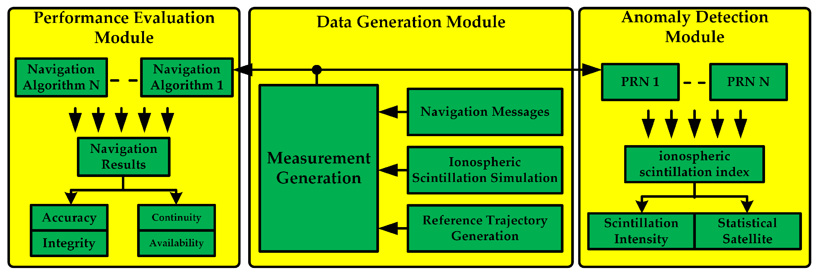
In Section 2.1.1, the ionospheric scintillation sequence is utilized to generate the pseudo-range and carrier-to-noise ratio values that are affected by the ionosphere. These values are then combined with the flight data, which are written in a file following a format similar to a RINEX file. This process enables the simulation of the GNSS system under various ionospheric scintillation intensities and during different flight phases.

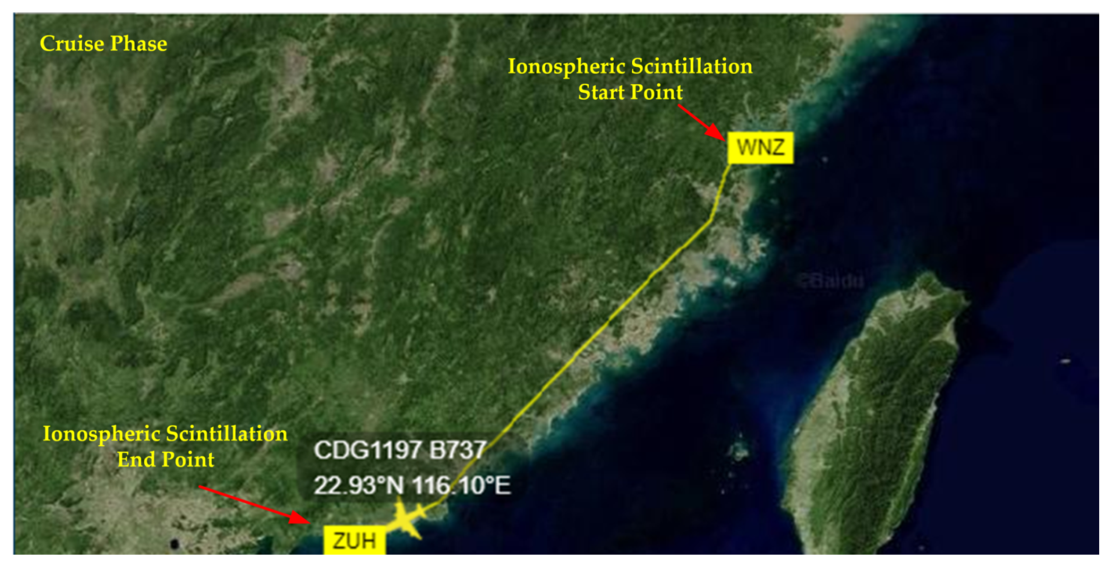
This paper employs the flight altitude as a criterion to categorize different flight phases, which helps to simulate the RINEX file based on flight data. The following classifications are used.

• Takeoff Phase: This phase is defined when the aircraft’s altitude is between 0 and 8000 m.
• Cruise Phase: The cruise phase is associated with altitudes of 8000 m and above.
• Approach Phase: When the aircraft’s altitude ranges between 1000 and 8000 m, it is considered the approach phase.
• Landing Phase: The landing phase refers to altitudes below 1000 m.

These divisions align with the ICAO categorization of flight segments into route, terminal, and approach phases [20]. By utilizing this classification, we can effectively simulate the RINEX file based on flight data, allowing for the comprehensive analysis and evaluation of GNSS performance in various flight phases.

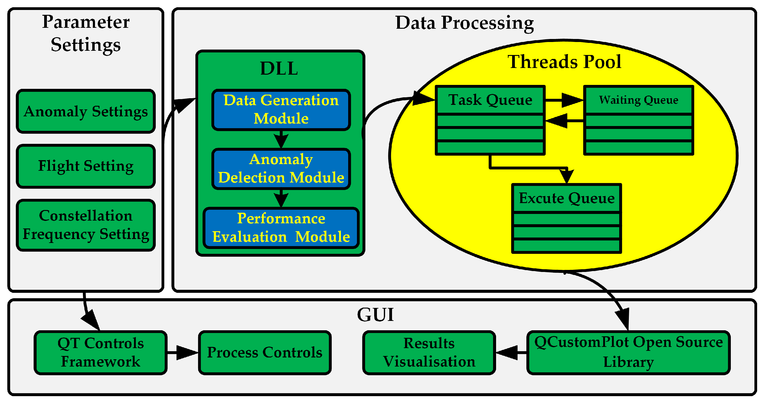
The flow of the software data generation module is shown in Figure 3. The software first calculates the position of the current visible satellite by using ephemeris data. It then combines the flight track data to obtain the distance between the satellite and the vehicle. After correcting for the Earth’s rotation, the software determines the actual distance between the satellite and the vehicle. Using the ionospheric scintillation simulation module, the software generates the amplitude scintillation sequence and converts it into a delay to obtain the pseudo-distance information affected by the ionospheric scintillation. The simulated carrier-to-noise ratio is determined by the free loss, atmospheric loss, and receiver antenna gain. In the ideal condition, the free loss represents the maximum loss in satellite signal propagation. To calculate the residual amount of the free loss, the actual distance of the satellite is subtracted from the farthest distance of the satellite. By adding the minimum receiving strength to the residual amount of the free loss, the ideal receiver receiving strength is obtained. The ionospheric scintillation simulation module is used to obtain the phase scintillation sequences. Finally, the software combines the phase scintillation sequence and the ionospheric scintillation simulation module to determine the carrier-to-noise ratio of the satellite under ionospheric scintillation.

2.2. Anomaly Detection Module

Once the RINEX file has been acquired through the method outlined in Section 2.1, the software will employ the carrier-to-noise ratio of the satellites to estimate the ionospheric scintillation index $S_4$. The RINEX file does not directly provide signal intensity data, but it does include the carrier-to-noise ratio. By leveraging the carrier-to-noise ratio and deriving an approximate signal intensity, we can effectively calculate the ionospheric scintillation index $S_4$, enabling the accurate detection of ionospheric scintillation phenomena [21].

Let the signal strength be $SI$ and the noise strength be $N_0$, and use $C/N_0$ to denote the signal-to-noise ratio $SI/N_0$ to obtain

$$SI/N_0={10}^{C{N}_0/10}$$

(10)

Let $S{I}_k$ represent the measured signal strength at time k, $S{I}_k^{\prime }$ represent the measured signal strength at time k after detrending, and $S{I}_k^{\prime \prime }$ represent the equivalent signal strength at time k after detrending derived from the signal-to-noise ratio.

$${S{I}_k}^{″}=\frac{(SI/N_0)}{{\sum }_{i=1}^{60/times{f}_s}{(SI/N_0)}_{k-i}/(60\times f_s)}$$

(11)

where $f_s$ is the sampling rate. With Equation (11), the receiver noise intensity N remains approximately constant each time $S_4$ is calculated [22].

$${S{I}_k}^{″}\approx {S{I}_k}^{\prime }=\frac{\left(S{I}_k\right)}{{\sum }_{i=1}^{60/times{f}_s}S{I}_{k-i}/(60\times f_s)}$$

(12)

Combining Equation (1) with Equation (12), $S_4$ can be approximated by the load-to-noise ratio in the RINEX file. The processing flow is shown in Figure 4.

In order to visualize the magnitude of the ionospheric scintillation intensity, the value of $S_4$ is therefore used to describe the ionospheric scintillation intensity. When $S_4=0$, it indicates the absence of ionospheric scintillation. When $S_4\le 0.3$, it indicates weak ionospheric scintillation. When $0.3<S_4\le 0.6$, it is classified as moderate ionospheric scintillation. When $S_4>0.6$, it denotes strong ionospheric scintillation. The software performs $S_4$ calculations for visible satellites in order to assess the prevailing intensity of ionospheric scintillation and to determine the number of satellites affected by it.

2.3. Performance Evaluation Module

The software will implement the navigation solution by utilizing the obtained RINEX file through the method outlined in Section 2.1, as shown in Figure 5. This process involves utilizing the pseudo-range in the observation file and the orbit parameters in the navigation message. By combining the results of the navigation solution with the performance evaluation algorithms, the software will calculate the accuracy, integrity, continuity, and availability of the GNSS system.

2.3.1. Calculation of Accuracy Indicators

Accuracy evaluation is the most basic and important indicator in the evaluation of aviation service performance. The accuracy of positioning services is related to the number of satellites and pseudo-range involved in the positioning solution, so the parameters related to accuracy mainly include the number of visible stars, positioning error, and dilution of precision (DOP).

1. Visible Stars and DOP. In the navigation solution module, the software automatically filters out satellites with a carrier-to-noise ratio below 35 dB and a satellite elevation angle less than 15 degrees. This is because the carrier-to-noise ratio significantly impacts the quality of the satellite signal. A lower carrier-to-noise ratio can result in poorer signal quality, which in turn affects the accuracy of the positioning. Similarly, satellites with a low elevation angle may also experience more interference, leading to decreased signal quality. By filtering out satellites that do not meet these criteria, the software selects satellites with better signal quality for position resolution. It has been observed that a larger number of satellites involved in positioning leads to improved accuracy. Therefore, maximizing the number of satellites used enhances the overall positioning accuracy.

The spatial distribution of satellites is known as the geometric configuration of the satellites and can be reflected by the DOP value. The software uses the DOP value to predict the positioning accuracy of the system, with smaller DOP values indicating higher positioning accuracy.

We calculate the weight coefficient matrix G using the observation matrix H defined in Equation (13).

$$G={\left(H^{T}H\right)}^{-1}=\left[\begin{array}{cccc}{G}_{11}& G_{12}& G_{13}& G_{14}\\ G_{21}& G_{22}& G_{23}& G_{24}\\ G_{31}& G_{32}& G_{33}& G_{34}\\ G_{41}& G_{42}& G_{43}& G_{44}\end{array}\right]$$

(13)

We can calculate the geometric dilution of precision (GDOP), position dilution of precision (PDOP), horizontal dilution of precision (HDOP), and vertical dilution of precision (VDOP) using matrix G:

$$\begin{array}{cc}& GDOP=\sqrt{G_{11}+G_{22}+G_{33}+G_{44}}\\ & PDOP=\sqrt{G_{11}+G_{22}+G_{33}}\\ \hfill & HDOP=\sqrt{G_{11}+G_{22}}\\ \hfill & VDOP=\sqrt{G_{33}}\end{array}$$

(14)

2. Position Errors. This reflects the accuracy of the navigation solution position and the user’s real position. In order to reflect the positioning error more intuitively, the software carries out statistical analysis of the positioning error from different dimensions, as shown in Figure 6.

One-dimensional metrics are used to assess the horizontal and vertical positioning errors. Of these, the root mean square (RMS) is used to describe the degree of dispersion of the positioning error and reflects the stability of the positioning service. In order to describe the positioning accuracy, we can rank the horizontal and vertical positioning errors in the evaluation period in ascending order and take the value ranked at 95% as the 95% positioning error. By comparing this with the performance requirements given by ICAO, we can determine whether the positioning accuracy meets the indicator requirements.

Two-dimensional metrics are computed based on the longitude and latitude, or the east and north components of the station’s central coordinate system. The 2DRMS is determined by the standard deviation of the error in both directions and is defined as the radius of the error circle that encloses the horizontal positioning errors. Circular error probable (CEP) represents the 50% equal probability error. If the user’s true position is at the center of the error circle, and the CEP is its radius, then the positioning results are dispersed within the circle with a 50% likelihood.

Three-dimensional metrics describe the result of the variation in the positioning results with direction through spherical error probable (SEP), with the user’s true position as the center of the sphere, and the user’s positioning results are distributed discrete within a sphere of radius SEP with an eccentricity of 50%.

2.3.2. Calculation of Integrity Indicators

Integrity evaluation plays a crucial role in ensuring the reliability of GNSS navigation positioning [23]. It is utilized to evaluate the accuracy of positioning and monitors real-time integrity risk events. Parameters such as the protection level (PL) and alert limit (AL), as well as the integrity risk probability, are employed in this evaluation process.

PL is a measure of the magnitude of the user positioning error and consists of two components in the horizontal and vertical directions. The magnitude of PL reflects the system ephemeris error and the geometric distribution of visible satellites, and it translates the error in the pseudo-range domain into an error in the positioning domain. In representing PL, a certain confidence probability can be used to define the error range, which allows a more accurate description of the positioning error and acts as an envelope [24]. The general form of PL is

$$PL=K•\sigma$$

(15)

$$K=\frac{1}{\sqrt{2\pi }}{\int }_{\frac{p}{2}}^{\infty }{e}^{-\frac{t^2}{2}}\mathrm{d}t$$

(16)

where K is the value corresponding to a certain confidence probability and $\sigma$ is the observed measurement error in the corresponding direction. By simplifying the observation equation, the following Equation (17) can be obtained.

$$y=Hx+\epsilon$$

(17)

In Equation (17), y represents the n-dimensional vector of the difference between the observed pseudo-range of the satellite and the estimated pseudo-range, n is the visible satellite, x denotes the four unknowns to be solved, and $\epsilon$ is the pseudo-range noise error. Based on the weighted least squares principle, the user solution $\widehat{x}$ is obtained:

$$\widehat{x}={\left(H^{T}WH\right)}^{-1}{H}^{T}Wy$$

(18)

where the weighted array W is

$$W=\left[\begin{array}{cccc}{\omega }_1& 0& \cdots & 0\\ 0& {\omega }_2& \cdots & 0\\ \cdots & \cdots & \cdots & \cdots \\ 0& \cdots & \cdots & {\omega }_i\end{array}\right]$$

(19)

In Equation (19), ${\omega }_i=1/{\sigma }_i^2$ and ${\sigma }_i^2$ is the sum of the squares of the errors for the i-th satellite. The covariance array consisting of the estimation errors is obtained from the weight array W.

$${\left(H^{T}WH\right)}^{-1}=\left[\begin{array}{cccc}{\sigma }_X^2& {\sigma }_{XY}& {\sigma }_{XZ}& {\sigma }_{XT}\\ {\sigma }_{XY}& {\sigma }_Y^2& {\sigma }_{YZ}& {\sigma }_{YT}\\ {\sigma }_{XZ}& {\sigma }_{YZ}& {\sigma }_Z^2& {\sigma }_{ZT}\\ {\sigma }_{XT}& {\sigma }_{YT}& {\sigma }_{ZT}& {\sigma }_T^2\end{array}\right]$$

(20)

The horizontal and vertical errors ${\sigma }_H$, ${\sigma }_V$ are obtained by Equation (20).

$$\begin{array}{cc}& {\sigma }_H=\sqrt{\frac{{\sigma }_X^2+{\sigma }_Y^2}{2}+\sqrt{\frac{{\sigma }_X^2-{\sigma }_Y^2}{2}+{\sigma }_{XY}^2}}\\ \hfill & {\sigma }_V=\sqrt{{\sigma }_Z^2}\end{array}$$

(21)

We calculate the horizontal protection level (HPL) and vertical protection level (VPL) from ${\sigma }_H$, ${\sigma }_V$:

$$\begin{array}{ccc}\hfill HPL& =& K_{H,PA}\times {\sigma }_H\hfill \\ \hfill VPL& =& K_{V,PA}\times {\sigma }_V\hfill \end{array}$$

(22)

where $K_{H,PA}$ is the quantile of the zero-mean Gaussian distribution with confidence probability $1.93\times {10}^{-8}$, taken as 6.0. $K_{V,PA}$ is the quantile of the zero-mean Gaussian distribution with confidence probability $9.82\times {10}^{-8}$, taken as 5.33.

The availability of integrity is determined by comparing PL with AL. For each positioning solution, PL is calculated in the above way and compared with AL at different flight phase performance indicators. If PL > AL, the completeness alarm mechanism will be triggered; otherwise, the system is ready to complete this phase.

2.3.3. Calculation of Continuity Indicators

The purpose of the continuity assessment is to reflect the number of continuity risk events that have occurred during the assessment cycle. In measuring the continuity risk, in addition to the failure of the positioning service to meet expected performance indicators, the detection of alarms in the event of satellite failure and false alarms in the event of no system failure are also taken into account.

The probability of continuity risk is determined by counting continuity events using a sliding window approach. A continuity event is counted when the system is initially available at the start of the assessment period but becomes unavailable (when the protection level crosses the alarm threshold) for at least one second within the sliding window length $T_{op}$. To calculate the probability of continuity risk, the number of continuity events is divided by the total number of samples available during the assessment period. This ratio between the number of continuity events and the total number of available samples in the evaluation period yields the probability of continuity risk $P_{CR}$.

$$P_{CR}=\frac{n_{Con}}{{\sum }_{t=t_{start,t=t+T}}^{t_{end-T_{op}}}\left\{Bool\left(t\right)\right\}}$$

(23)

In Equation ((23), $n_{Con}$) indicates the number of occurrences of continuity events, $t_{start}$ indicates the starting point of the evaluation, $t_{end}$ indicates the moment of completion of the evaluation, and T indicates the evaluation sampling interval.

2.3.4. Calculation of Availability Indicators

1. PDOP Availability. PDOP availability means that the value of PDOP meets the specified PDOP limits for a given time period. The constraint in the publicly available Service Performance Specification for service evaluation is PDOP ≤ 6.

2. Locating Service Availability. In order to visually analyze the availability of location services, an availability distribution diagram is created using the position errors (PE) as the horizontal axis and protect level (PL) as the vertical axis to depict the horizontal and vertical integrity risk distribution, as shown in Figure 7.

During the evaluation cycle, the current system service availability is judged based on the relationship between PE, PL, and AL. When PE < PL < AL, the system service meets the specified demand and the service is available. When PE < AL < PL or AL < PE < PL, the current service is not available. When AL < PL < PE or PL < PE < AL, it indicates that misleading information (MI) is generated. When PL < AL < PE, an integrity risk event is detected, in which hazardously misleading information (HMI) has occurred.

3. Implementation of the Software

The software implementation process is shown in Figure 8. The software utilizes the QT standard framework to design the software’s upper layer GUI, which allows for parameter settings. The underlying task function is implemented using the C/C++ language. To encapsulate and manage the task function, dynamic link libraries and thread pools are utilized. Lastly, the QCustomplot open-source plotting library is used to visualize the final evaluation results.

3.1. Parameter Settings

Figure 9 shows the parameter configuration interface based on the QT framework. The settings module, located on the left-hand side, facilitates a variety of adjustments, encompassing crucial details such as data sources, performance evaluation criteria, constellation types, and frequency points. Furthermore, the ionospheric anomaly setting function enables users to modify the strength and duration of ionospheric scintillation. Additionally, users can specify the corresponding flight number and flight stage through the flight plan settings.

3.2. Data Processing

3.2.1. Encapsulation of Task Modules with Dynamic Link Libraries

The software encapsulates complex data processing modules into dynamic link libraries (DLLs). When the software is executed, the address of the function is identified through a global offset table in the DLL, allowing the call to be completed [25]. The use of DLLs eliminates the need for multiple copies of the library in the memory, which would be required with static linking. In cases where multiple programs rely on the same library, dynamic linking only requires one copy of the library to be stored in the memory, thus saving memory space. Furthermore, dynamic linking simplifies the process of program updates. Instead of having to relink all the programs, only the original target file needs to be replaced when updating a library. This means that when the program is executed again, the updated version of the target file is automatically loaded into the memory and linked to the program, allowing for seamless program upgrades. Therefore, encapsulating the complex data processing module as a DLL has significant advantages in improving memory utilization and facilitating program updates [26].

3.2.2. Managing Task Modules with Thread Pool

Thread pooling is a technique used to manage threads, and it involves initializing and creating a specific number of threads when the program is started. This thread pool is responsible for selecting an idle thread from the pool to handle a task whenever it needs to be executed. After the task module is executed, instead of destroying the thread, it is returned to the thread pool. By encapsulating the data generation module, exception detection, and performance evaluation module in the form of dynamic link libraries, the program’s memory utilization is improved, and it becomes easier to update the iterative version. Moreover, these dynamic link libraries can be shared among different threads, as shown in Figure 10. Utilizing a thread pool helps to avoid the overhead associated with frequently creating and destroying threads, while also improving the thread reuse and execution efficiency [27].

3.3. GUI Part

The implementation principle is shown in Figure 11. The software provides users with flight monitoring functions, including anomaly detection, performance evaluation, and querying flight information and flight trajectories through the FlightAware API. It also generates satellite maps using HTML and processes flight trajectory data in JavaScript. The processed data are then communicated with the GUI interface through QWebChannel. The GUI module processes the flight information to support the display of the flight’s start and end points, as well as the adjustment of the trajectory simulation speed and flight detail querying.

The software enables the real-time monitoring of the flight track, allowing users to freely control the playback speed for better observation of the aircraft’s flight. Additionally, the software offers detailed aircraft information and real-time data, allowing users to easily obtain important information such as the exact starting moment and current latitude, longitude, altitude, and speed of the aircraft. The flight track monitoring and observation function of flight CES2513 from Wuhan International Airport (WUH) to Shanghai Pudong Airport (SHA) is shown in Figure 12.

4. Analysis of Evaluation Results

This section selects the cruise phase and the approach phase of the four flight phases as the test cases. Ionospheric scintillation effects are likely to occur in the equatorial and mid-latitudes. Therefore, this paper chooses two flight routes in the low-latitude region and mid-latitude region, namely flight number CDG1197 (Wenzhou to Zhuhai) and flight number UAL235 (Berlin to Washington).

4.1. Cruise Phase Evaluation

Evaluation of GNSS System Performance during the Cruise Phase: Scintillation-Free and Strong Ionospheric Scintillation Environments. In this section, the aviation service performance evaluation software was utilized to evaluate the performance of the GNSS system during the cruise phase. The specific test flight segment selected for evaluation was the route from WenZhou to ZhuHai, with the flight number CDG1197, and Berlin to Washington, with flight number UAL235. The trajectory of the cruise phase can be observed in Figure 13 and Figure 14. To assess the impact of ionospheric scintillation, the software’s parameter setting window, as depicted in Figure 9, was utilized. The ionospheric scintillation interference was set to a strong scintillation level, covering the entire duration of the cruise phase, from its commencement to its conclusion. The results of the air service performance evaluation during the designated evaluation cycle are illustrated in Figure 15, Figure 16, Figure 17 and Figure 18 and

Table 1. A comparative analysis of GPS L1 accuracy performance in scintillation-free and strong ionospheric scintillation environments during the cruise phase in CDG1197.

Accuracy Indicators	Without Ionospheric Scintillation	Strong Ionospheric Scintillation
Horizontal Error (m, 95%)	1.17	3.62
Vertical Error (m, 95%)	6.39	8.80
Horizontal RMS (m)	0.32	1.08
Vertical RMS (m)	1.24	1.87
Availability (%)	100	100
CEP (m, 95%)	1.91	3.62

,

Table 2. A comparative analysis of GPS L1 accuracy performance in scintillation-free and strong ionospheric scintillation environments during the cruise phase in UAL235.

Accuracy Indicators	Without Ionospheric Scintillation	Strong Ionospheric Scintillation
Horizontal Error (m, 95%)	1.65	5.02
Vertical Error (m, 95%)	5.21	6.04
Horizontal RMS (m)	0.86	1.89
Vertical RMS (m)	1.14	1.54
Availability (%)	100	100
CEP (m, 95%)	1.96	4.75

,

Table 3. A comparative analysis of GPS L1 integrity performance in scintillation-free and strong ionospheric scintillation environments during the cruise phase in CDG1197.

Integrity Indicators	Without Ionospheric Scintillation	Strong Ionospheric Scintillation
HPL (m)	24	38
VPL (m)	53	55
Availability (%)	100	100
M#1 (%)	0	0
HMI (%)	NULL	NULL

and

Table 4. A comparative analysis of GPS L1 integrity performance in scintillation-free and strong ionospheric scintillation environments during the cruise phase in UAL235.

Integrity Indicators	Without Ionospheric Scintillation	Strong Ionospheric Scintillation
HPL (m)	198	610
VPL (m)	126	229
Availability (%)	100	100
M#1 (%)	0	0
HMI (%)	NULL	NULL

.

Figure 15 and Figure 16 show a comparison of the accuracy evaluation for GPS L1 during the cruise phases of flight CDG1197 and flight UAL235 in both an environment without ionospheric scintillation and a strongly ionospheric environment. The accuracy metrics are referenced to the standards specified by the ICAO for the prescribed route phase.

Table 1 shows the positioning accuracy indexes under different ionospheric scintillation intensities in CDG1197, from which it can be seen that the airborne GNSS system loses 196.58% and 37.72% of its accuracy in the horizontal and vertical 95% positioning errors under strong ionospheric scintillation compared with that in the no ionospheric scintillation environment, respectively. The horizontal and vertical RMS increases by 237.5% and 50.81% under strong ionospheric scintillation compared to the scintillation-free environment, and the DOP value shows irregular jitter compared to the scintillation-free environment, with the maximum value of PDOP being 4.17. The circular probability error loses 89.52% of its accuracy under strong ionospheric scintillation compared to the scintillation-free environment. The availability is 100% in both the scintillation-free and strong scintillation environments, which indicates that GPS L1 meets the accuracy specifications for the route phase during the cruise phase.

Table 3 shows the positioning accuracy indexes under different ionospheric scintillation intensities in UAL235, from which it can be seen that the airborne GNSS system loses 204.2% and 15.93% of its accuracy in the horizontal and vertical 95% positioning errors under strong ionospheric scintillation compared with that in the no ionospheric scintillation environment, respectively. The horizontal and vertical RMS increases by 119.7% and 35.08% under strong ionospheric scintillation compared to the scintillation-free environment, and the DOP value shows irregular jitter compared to the scintillation-free environment, with the maximum value of PDOP being 6.19. The circular probability error loses 142.34% of its accuracy under strong ionospheric scintillation compared to the scintillation-free environment. The availability is 100% in both the scintillation-free and strong scintillation environments, which indicates that GPS L1 meets the accuracy specifications for the route phase during the cruise phase.

Figure 17 and Figure 18 show a comparison of the integrity evaluation for GPS L1 during the cruise phases of flight CDG1197 and flight UAL235 in both an environment without ionospheric scintillation and a strongly ionospheric environment. The integrity metrics are referenced to the standards specified by the ICAO for the prescribed route phase.

Table 4 shows the integrity metrics at different ionospheric scintillation intensities in CDG1197. From the table, it can be seen that when the ionospheric scintillation intensity increases, the maximum HPL and VPL of the airborne GNSS system increase by 58.33% and 3.82% relative to the environment without ionospheric scintillation. This indicates that under a strong ionospheric scintillation intensity, the positioning accuracy starts to deteriorate and a larger protection level is required to ensure that the system meets the performance requirements. Regardless of the ionospheric scintillation environment, the integrity availability of the GPS L1 system during the cruise phase meets the ICAO-defined performance requirements for the route phase.

Table 2 shows the integrity metrics at different ionospheric scintillation intensities in UAL235. From the table, it can be seen that when the ionospheric scintillation intensity increases, the maximum HPL and VPL of the airborne GNSS system increase by 208.08% and 81.746% relative to the environment without ionospheric scintillation. This indicates that under a strong ionospheric scintillation intensity, the positioning accuracy starts to deteriorate and a larger protection level is required to ensure that the system meets the performance requirements. The complete availability of the GPS L1 system during the cruise phase under strong ionospheric scintillation conditions does not meet the performance requirements for the route phase in compliance with the ICAO regulations.

4.2. Approach Phase Evaluation

For the approach phase, the performance of the BDS B1 system and GPS L1 system in an environment without ionospheric scintillation and in a strong ionospheric scintillation environment is evaluated in the Air Service Performance Evaluation Software. The flight trajectory of the approach phase is shown in Figure 19 and Figure 20. Through the parameter setting window as shown in Figure 9, the ionospheric scintillation interference is set to strong scintillation, and the duration is from the onset of the approach to the time that the vehicle slides into the airport runway. The results of the air service performance evaluation during the evaluation cycle are shown in Figure 21, Figure 22, Figure 23 and Figure 24 and

Table 5. A comparative analysis of BDS B1 accuracy performance in scintillation-free and strong ionospheric scintillation environments during the approach phase in CDG1197.

Accuracy Indicators	Without Ionospheric Scintillation	Strong Ionospheric Scintillation
Horizontal Error (m, 95%)	0.60	2.06
Vertical Error (m, 95%)	1.70	4.92
Horizontal RMS (m)	0.22	0.72
Vertical RMS (m)	1.19	1.66
Availability (%)	100	99.61
CEP (m, 95%)	1.73	2.91

,

Table 6. A comparative analysis of GPS L1 accuracy performance in scintillation-free and strong ionospheric scintillation environments during the approach phase in UAL235.

Accuracy Indicators	Without Ionospheric Scintillation	Strong Ionospheric Scintillation
Horizontal Error (m, 95%)	6.77	7.35
Vertical Error (m, 95%)	2.55	2.70
Horizontal RMS (m)	0.49	1.09
Vertical RMS (m)	1.40	1.76
Availability (%)	100	99.899
CEP (m, 95%)	2.31	1.95

,

Table 7. A comparative analysis of BDS B1 integrity performance in scintillation-free and strong ionospheric scintillation environments during the approach phase in CDG1197.

Integrity Indicators	Without Ionospheric Scintillation	Strong Ionospheric Scintillation
HPL (m)	11	13
VPL(m)	26.8	27.2
Availability (%)	0	0
M#1 (%)	0	0
M#2 (%)	0.193	0.193
HMI (%)	NULL	NULL

and

Table 8. A comparative analysis of GPS L1 integrity performance in scintillation-free and strong ionospheric scintillation environments during the approach phase in UAL235.

Integrity Indicators	Without Ionospheric Scintillation	Strong Ionospheric Scintillation
HPL (m)	35	66
VPL(m)	50	88
Availability (%)	0	0
M#1 (%)	0	0
M#2 (%)	0.101	0.101
HMI (%)	NULL	NULL

.

Figure 21 and Figure 22 show a comparison of the accuracy evaluation for BDS B1 and GPS L1 during the approach phases of flight CDG1197 and flight UAL235 in both an environment without ionospheric scintillation and a strongly ionospheric environment. The accuracy metrics are referenced to the standards specified by the ICAO for the prescribed approach phase.

Table 5 shows the positioning accuracy indexes under different ionospheric scintillation intensities, from which it can be seen that the airborne GNSS system loses 243.33% and 189.41% of its accuracy in the horizontal and vertical 95% positioning errors under strong ionospheric scintillation compared with that in the no ionospheric scintillation environment, respectively. The horizontal and vertical RMS increases by 227.3% and 39.49% under strong ionospheric scintillation compared to the scintillation-free environment, and the DOP value shows irregular jitter compared to the scintillation-free environment, with the maximum value of PDOP being 1.76. The circular probability error loses 68.21% of its accuracy under strong ionospheric scintillation compared to the scintillation-free environment. During the approach phase, the accuracy performance of BDS B1 in a non-ionospheric scintillation environment meets the ICAO standard for precision approach category I. The availability in a strong ionospheric scintillation environment is 99.614%, which does not meet the ICAO standard for precision approach category I.

Table 6 shows the positioning accuracy indexes under different ionospheric scintillation intensities, from which it can be seen that the airborne GNSS system loses 8.68% and 5.98% of its accuracy in the horizontal and vertical 95% positioning errors under strong ionospheric scintillation compared with that in the no ionospheric scintillation environment, respectively. The horizontal and vertical RMS increases by 122.44% and 25.71% under strong ionospheric scintillation compared to the scintillation-free environment, and the DOP value shows irregular jitter compared to the scintillation-free environment, with the maximum value of PDOP being 3.04. During the approach phase, the accuracy performance of GPS L1 in a non-ionospheric scintillation environment meets the ICAO standard for precision approach category I. The availability in a strong ionospheric scintillation environment is 99.899%, which does not meet the ICAO standard for precision approach category I.

Figure 23 and Figure 24 show a comparison of the accuracy evaluation for BDS B1 and GPS L1 during the approach phases of flight CDG1197 and flight UAL235 in both an environment without ionospheric scintillation and a strongly ionospheric environment. The integrity metrics are referenced to the standards specified by the ICAO for the prescribed approach phase.

Table 7 and Table 8 show the integrity metrics at different ionospheric scintillation intensities. It can be seen from the tables that the maximum HPL and VPL of the airborne GNSS system fluctuate when the ionospheric scintillation intensity increases relative to the non-ionospheric scintillation environment. Regardless of the ionospheric scintillation environment, in the approach phase, the horizontal integrity availability of the BDS B1 system and GPS L1 system meets the ICAO-defined precision approach category I performance requirements, while the vertical integrity fails to meet the ICAO-defined precision approach category I performance requirements both in CDG1197 and UAL235.

5. Conclusions and Further Studies

This paper presents a GNSS aviation service performance evaluation software program, which is designed based on the ionospheric scintillation model and satellite navigation principles. The software is flexible and can be applied to different ionospheric scintillation intensities. To verify the feasibility of the proposed design approach, the software assesses the performance of GNSS aviation services’ different routes and ionospheric scintillation intensities. The simulation results indicate that, even in the presence of strong ionospheric scintillation, the GPS L1 system successfully meets the ICAO performance requirements, specifically during the cruise phase of route navigation. On the other hand, the BDS B1 system, which is affected by strong ionospheric scintillation, fulfills the ICAO horizontal integrity requirements for precision approach category I during the approach phase, but does not meet the precision and vertical integrity requirements. Furthermore, the performance of the GNSS systems under ionospheric scintillation conditions tends to be consistent in the mid- and low-latitude regions, which validates the feasibility of the software. To further evaluate the performance of each flight phase in the presence of strong ionospheric scintillation, future studies will expand the scope of evaluation to incorporate additional joint navigation routes.

References

1. Chiou, T.Y.; Seo, J.; Walter, T.; Enge, P. Performance of a Doppler-aided GPS navigation system for aviation applications under ionospheric scintillation. In Proceedings of the 26th International Technical Meeting of the Satellite Division of The Institute of Navigation (ION GNSS+ 2013), Nashville, TN, USA, 16–20 September 2008; pp. 1139–1147. [Google Scholar]
2. Wang, N.; Li, Z.; Huo, X.; Li, M.; Yuan, Y.; Yuan, C. Refinement of global ionospheric coefficients for GNSS applications: Methodology and results. Adv. Space Res. 2019, 63, 343–358. [Google Scholar] [CrossRef]
3. Pullen, S.; Opshaug, G.; Hansen, A.; Walter, T.; Enge, P.; Parkinson, B. A preliminary study of the effect of ionospheric scintillation on WAAS user availability in equatorial regions. In Proceedings of the 11th International Technical Meeting of the Satellite Division of The Institute of Navigation (ION GPS 1998), Nashville, TN, USA, 15–18 September 1998; pp. 687–699. [Google Scholar]
4. Ruan, H.; Zhang, L.; Luo, Y.; Long, T. GNSS Carrier Phase Tracking with Discrete Wavelet Transform Filtering under Ionospheric Scintillation. IEEE Commun. Lett. 2017, 21, 394–397. [Google Scholar] [CrossRef]
5. Humphreys, T.E.; Psiaki, M.L.; Hinks, J.C.; O’Hanlon, B.; Kintner, P.M. Simulating ionosphere-induced scintillation for testing GPS receiver phase tracking loops. IEEE J. Sel. Top. Signal Process. 2009, 3, 707–715. [Google Scholar] [CrossRef]
6. Humphreys, T.E.; Psiaki, M.L.; Kintner, P.M. Modeling the effects of ionospheric scintillation on GPS carrier phase tracking. IEEE Trans. Aerosp. Electron. Syst. 2010, 46, 1624–1637. [Google Scholar] [CrossRef]
7. Garcia-Pena, A.; Macabiau, C.; Julien, O.; Mabilleau, M.; Durel, P. IGNSS Computation Models and Values for GPS and GALILEO L5/E5a Civil Aviation Receivers. In Proceedings of the 33rd International Technical Meeting of the Satellite Division of The Institute of Navigation (ION GNSS+ 2020), Online, 22–25 September 2020; pp. 206–218. [Google Scholar]
8. Pericacho, J.G.; Celada, J.; Sánchez, D.; Janicki, K.W.; Díaz, F.; Quiles, X.; Arribas, V.; Andrés, J.; de Echazarreta, C.L. PROARAIM: Towards the early adoption of ARAIM air navigation services. In Proceedings of the 34th International Technical Meeting of the Satellite Division of The Institute of Navigation (ION GNSS+ 2021), Online, 20–24 September 2021; pp. 1160–1175. [Google Scholar]
9. Jan, S.S.; Chan, W.; Walter, T. MATLAB algorithm availability simulation tool. GPS Solut. 2009, 13, 327–332. [Google Scholar] [CrossRef]
10. GSSF Team. Galileo System Simulation Facility–Algorithms and Models; Technical Report; VEGA Group PLC: Darmstadt, Germany, 2004. [Google Scholar]
11. Leandro, R.F.; Santos, M.C.; Langley, R.B. Analyzing GNSS data in precise point positioning software. GPS Solut. 2011, 15, 1–13. [Google Scholar] [CrossRef]
12. Kim, H.; Lee, J.; Oh, S.H.; So, H.; Hwang, D.H. Multi-radio integrated navigation system M&S software design for GNSS backup under navigation warfare. Electronics 2019, 8, 188. [Google Scholar] [CrossRef]
13. ICAO. Annex 10—Aeronautical Telecommunications Volume I: Radio Navigation Aids, 7th ed.; ICAO: Montreal, ON, Canada, 2018. [Google Scholar]
14. Tang, A.; Aleti, A.; Burge, J.; van Vliet, H. What makes software design effective? Des. Stud. 2010, 31, 614–640. [Google Scholar] [CrossRef]
15. Jiao, Y.; Morton, Y.T. Comparison of the effect of high-latitude and equatorial ionospheric scintillation on GPS signals during the maximum of solar cycle 24. Radio Sci. 2015, 50, 886–903. [Google Scholar] [CrossRef]
16. Xu, C.Y.; Ni, S. Performance Analysis of Different CN0 Estimation Algorithms under Ionospheric Scintillation. GNSS World China 2016, 41, 602–611. [Google Scholar] [CrossRef]
17. Lu, S.; Xing, Z.; Deng, Z. Modelling research on the relationship between ionospheric scintillation index and drift speed in the polar ionosphere. Chin. J. Geophys. 2022, 65, 3704–3713. [Google Scholar]
18. Sun, P.Y.; Huang, Y.; Tang, X. Simulating and analyzing the impact of ionospheric scintillation for BeiDou navigation signals. J. Natl. Univ. Def. Technol. 2016, 38, 111–116. [Google Scholar]
19. Gałdyn, F.; Zajdel, R.; Sośnica, K. RINEXAV: GNSS global network selection open-source software based on qualitative analysis of RINEX files. SoftwareX 2023, 22, 101372. [Google Scholar] [CrossRef]
20. Wang, P.; Zhang, Y.; Liu, J. A flight phase identification method based on airborne data for civil aircraft. J. Traffic Transp. Eng. 2022, 22, 216–228. [Google Scholar] [CrossRef]
21. Sun, W.J.; Jing, S. An adaptive carrier-to-noise ratio estimation method for GNSS weak signal. J. Beijing Univ. Aeronaut. Astronaut. 2021, 47, 2068–2074. [Google Scholar] [CrossRef]
22. Bhuiyan, M.Z.H.; Söderholm, S.; Thombre, S.; Ruotsalainen, L.; Kirkko-Jaakkola, M.; Kuusniemi, H. Performance Evaluation of Carrier-to-Noise Density Ratio Estimation Techniques for BeiDou B1 Signal. In Proceedings of the 2014 Ubiquitous Positioning Indoor Navigation and Location Based Service (UPINLBS), Corpus Christ, TX, USA, 20–21 November 2014. [Google Scholar] [CrossRef]
23. Yang, L.; Fu, Y.; Zhu, J.; Shen, Y.; Rizos, C. Overbounding residual zenith tropospheric delays to enhance GNSS integrity monitoring. GPS Solut. 2023, 27, 76. [Google Scholar] [CrossRef]
24. Li, L.; Li, R.; Wang, L.; Wang, R.; Li, M.; Li, M. GNSS integrity risk evaluation in position domain based on the generalized Pareto distribution. Meas. Sci. Technol. 2023, 34, 095010. [Google Scholar] [CrossRef]
25. Wu, Z.; Wang, H.; Zhang, Y.; Ai, M. ABB robot data collection based on dynamic link library. J. Phys. Conf. Ser. 2021, 2113, 012077. [Google Scholar] [CrossRef]
26. Wang, W.-X.; Gao, Q.; Xu, K.; Zhang, S.-K. Crash Input Classification Method Combined with Dynamic Link Library Information. J. Softw. 2023, 34, 1594–1612. [Google Scholar] [CrossRef]
27. Shoshany, B. A C++ 17 Thread Pool for High-Performance Scientific Computing. arXiv 2021, arXiv:2105.00613. [Google Scholar]
Figure 1. Software system architecture.
Electronics 12 03713 g001
Figure 2. Obtaining ionospheric scintillation sequences using the Cornell model.
Electronics 12 03713 g002
Figure 3. Data generation module process.
Electronics 12 03713 g003
Figure 4. Anomaly detection module process.
Electronics 12 03713 g004
Figure 5. Performance evaluation module process.
Electronics 12 03713 g005
Figure 6. Positioning error indicators in three dimensions.
Electronics 12 03713 g006
Figure 7. Location service availability distribution.
Electronics 12 03713 g007
Figure 8. Software design process.
Electronics 12 03713 g008
Figure 9. Parameter setting interface in software.
Electronics 12 03713 g009
Figure 10. The principles of a thread pool.
Electronics 12 03713 g010
Figure 11. Flight monitoring system design process.
Electronics 12 03713 g011
Figure 12. GUI for flight monitoring system.
Electronics 12 03713 g012
Figure 13. Reference trajectory for performance evaluation (CDG1197) in Cruise Phase.
Electronics 12 03713 g013
Figure 14. Reference trajectory for performance evaluation (UAL235) in Cruise Phase.
Electronics 12 03713 g014
Figure 15. Display of GPS L1 accuracy evaluation results (CDG1197) within the software interface.
Electronics 12 03713 g015
Figure 16. Display of GPS L1 accuracy evaluation results (UAL235) within the software interface.
Electronics 12 03713 g016
Figure 17. Display of GPS L1 integrity evaluation results (CDG1197) within the software interface.
Electronics 12 03713 g017
Figure 18. Display of GPS L1 integrity evaluation results (UAL235) within the software interface.
Electronics 12 03713 g018
Figure 19. Reference trajectory for performance evaluation (CDG1197) in Approach Phase.
Electronics 12 03713 g019
Figure 20. Reference trajectory for performance evaluation (UAL235) in Approach Phase.
Electronics 12 03713 g020
Figure 21. Display of BDS B1 accuracy evaluation results (CDG1197) within the software interface.
Electronics 12 03713 g021
Figure 22. Display of GPS L1 accuracy evaluation results (UAL235) within the software interface.
Electronics 12 03713 g022
Figure 23. Display of BDS B1 integrity evaluation results (CDG1197) within the software interface.
Electronics 12 03713 g023
Figure 24. Display of GPS L1 integrity evaluation results (UAL235) within the software interface.
Electronics 12 03713 g024