RSLC-Deeplab: A Ground Object Classification Method for High-Resolution Remote Sensing Images

Abstract

With the continuous advancement of remote sensing technology, the semantic segmentation of different ground objects in remote sensing images has become an active research topic. For complex and diverse remote sensing imagery, deep learning methods have the ability to automatically discern features from image data and capture intricate spatial dependencies, thus outperforming traditional image segmentation methods. To address the problems of low segmentation accuracy in remote sensing image semantic segmentation, this paper proposes a new remote sensing image semantic segmentation network, RSLC-Deeplab, based on DeeplabV3+. Firstly, ResNet-50 is used as the backbone feature extraction network, which can extract deep semantic information more effectively and improve the segmentation accuracy. Secondly, the coordinate attention (CA) mechanism is introduced into the model to improve the feature representation generated by the network by embedding position information into the channel attention mechanism, effectively capturing the relationship between position information and channels. Finally, a multi-level feature fusion (MFF) module based on asymmetric convolution is proposed, which captures and refines low-level spatial features using asymmetric convolution and then fuses them with high-level abstract features to mitigate the influence of background noise and restore the lost detailed information in deep features. The experimental results on the WHDLD dataset show that the mean intersection over union (mIoU) of RSLC-Deeplab reached 72.63%, the pixel accuracy (PA) reached 83.49%, and the mean pixel accuracy (mPA) reached 83.72%. Compared to the original DeeplabV3+, the proposed method achieved a 4.13% improvement in mIoU and outperformed the PSP-NET, U-NET, MACU-NET, and DeeplabV3+ networks.

1. Introduction

High-resolution remote sensing images contain rich geographic information and have many potential applications in areas including agricultural monitoring, land use, and urban planning [1,2], making the intelligent analysis of remote sensing images a topic of considerable interest. The semantic segmentation of remote sensing images is a significant image processing task [3,4], aiming to categorize each pixel and mark it as the corresponding category [5]. Remote sensing images are characterized by high quantities, complex backgrounds, and large scale changes. The process of manually annotating data is labor-intensive and prone to error. The rapid and accurate automatic extraction of object information from remote sensing images has become an urgent need.

There are three main semantic segmentation methods used for remote sensing images: traditional methods, machine learning, and deep learning. In the early days, traditional remote sensing image segmentation mostly relied on shallow features of the image, including the texture, edges, and geometric shapes of the target. Common segmentation methods based on image pixels include thresholding, edge detection, and region-based segmentation. Cuevas et al. [6] presented an automatic image segmentation approach that implements multi-thresholding through differential evolution optimization. This method is capable of dynamically selecting optimal thresholds while maintaining the primary features of the original image. Chen et al. [7] employed the Canny edge detector for edge detection on multispectral images and performed multi-scale segmentation on the detected edge features. The integration of edge information and segmentation scale effectively controlled the merging procedure of neighboring image objects. Byun et al. [8] achieved initial segmentation through an improved seed region-growing program and obtained segmentation results using a region adjacency graph to merge regions. To cope with complex remote sensing image segmentation scenarios, the simple linear iterative clustering (SLIC) superpixel segmentation algorithm, which utilizes the K-means clustering algorithm, is widely utilized in the remote sensing field. Csillik et al. [9] used SLIC superpixels to quickly segment and classify remote sensing data. Model-based segmentation methods based on Markov random fields are also widely used, which improve segmentation accuracy by introducing contextual information. Sziranyi et al. [10] applied unsupervised clustering to fused image series using cross-layer similarity measures and then performed multi-layer Markov random field segmentation. To overcome the constraints of single shallow-feature-based segmentation approaches, hybrid feature combination segmentation methods have been proposed, such as combining edge detection with region-based segmentation to enhance the quality of the segmentation outcomes. Zhang et al. [11] introduced a hybrid approach to region merging. This method utilizes the globally most similar region to establish the initial point for region growing and enhances the optimization ability for local region merging. These traditional methods rely too heavily on shallow features of the image, and pixel features are easily affected by factors such as the lighting, the presence of clouds and fog, and the sensors, resulting in insufficient reliability. The ability of machine learning to learn features and geometric relationships between images has received attention. Mitra et al. [12] used the support vector machine (SVM) algorithm to solve the problem of insufficient labeled pixels required for supervised pixel classification in remote sensing images. Bruzzone et al. [13] introduced an enhanced support-vector-machine-based semi-supervised approach for remote sensing image classification. By leveraging both labeled and unlabeled samples, this method effectively tackles the ill-posed problem. Pal et al. [14] used a random forest classifier to select the best category. Mellor et al. [15] used a random forest classification model to classify forest cover areas on multispectral remote sensing images. These methods heavily rely on handcrafted features, which result in a poor generalization capability [16,17].

With a high-resolution background, due to the impact of the spatiotemporal environment, objects of the same type present different spectral features, and the utilization of shallow features is inadequate for capturing the complexity of remote sensing images, thereby leading to limited segmentation accuracy. Deep learning methods have begun to attract attention as computing power has improved rapidly, since deep neural networks can automatically learn features in large datasets and extract deep semantic features of images, showing excellent performance. Classic segmentation models have begun to emerge. Long et al. [18] pioneered the fully convolutional network (FCN) semantic segmentation model, enabling pixel-level image classification. In a FCN, the traditional fully connected layer in the final layer of the network is replaced by a convolutional layer, allowing the network to accept inputs of arbitrary sizes and produce feature maps of the same size as the input. Zhong et al. [19] used an FCN to extract buildings and roads, which could better capture ground target features compared to traditional neural networks, but the eight-fold upsampling method lost image detail information. A series of segmentation networks using an encoder–decoder structure have been proposed, such as SegNet [20] and U-Net [21]. Cao et al. [22] proposed the Res-UNet network, which addresses the problems of gradient vanishing and feature loss in deep neural networks by introducing residual connections. Although it has achieved high segmentation accuracy in high-resolution remote sensing forest images, its segmentation performance for small target tree species is poor. Based on U-Net, Li et al. proposed MACU-Net [23], which utilizes asymmetric convolutions to replace regular convolutions and enhance the feature extraction capability, thus improving the utilization rate of features, but the segmentation of ground object boundaries is still not clear enough. To avoid reducing the size of the receptive field when obtaining feature maps at various scales, the utilization of dilated convolution [24] to perform convolution operations on input images is widespread. PSPNet [25] is a model based on pyramid pooling that implements the pyramid pooling module at the last layer to extract contextual information at different scales. DeeplabV1 was proposed in [26], which utilizes dilated convolution to perform convolution operations on input images in VGG [27] and then adds a conditional random field (CRF) module at the output end for post-processing to obtain relatively accurate contours. In DeeplabV2 [28], dilated convolutions are extensively applied to feature maps at multiple scales to capture contextual information at different levels, thereby improving segmentation accuracy. DeeplabV3 [29] optimized the ASPP module by adding average pooling and batch normalization operations to improve the feature representation and model generalization capabilities. Removing the CRF as a post-processing module still achieved good segmentation results. DeeplabV3+ [30] included a decoder module to fuse shallow features in the encoder with deep features output by the encoder in order to further optimize the edges and details of the segmentation results. Compared with classical semantic segmentation methods, DeeplabV3+ can segment ground objects in complex remote sensing images, but it still faces challenges such as the inaccurate segmentation of small targets and blurred boundary information. Wang et al. [31] introduced a class feature attention mechanism into the DeeplabV3+ network to enhance the correlation between different categories and effectively extract and process semantic information of diverse categories.

The attention mechanism holds great importance in the field of deep learning. It can assist a model in identifying useful information within the input data, suppressing irrelevant information, and enhancing performance and efficiency. SENet [32] assigns different weights to each channel by learning the correlation between feature channels. The Efficient Channel Attention Network (ECA-Net) [33] models the interactions between convolutional feature channels and introduces an adaptive channel attention mechanism, optimizing the negative impact of dimensionality reduction in SENet. To account for information interaction in the spatial dimension, Woo et al. [34] introduced the Convolutional Block Attention Module (CBAM), which uses a channel attention module and a spatial attention module in series to perform adaptive feature refinement, in contrast to methods that employ costly and complex techniques such as non-local or self-attention blocks. The Coordinate Attention (CA) mechanism [35] encodes each spatial position, which aids in capturing global contextual information and long-range dependencies. It proves particularly effective for remote sensing images, where spatial relationships and geometric information play a crucial role, enabling neural networks to better comprehend input data and improve prediction accuracy.

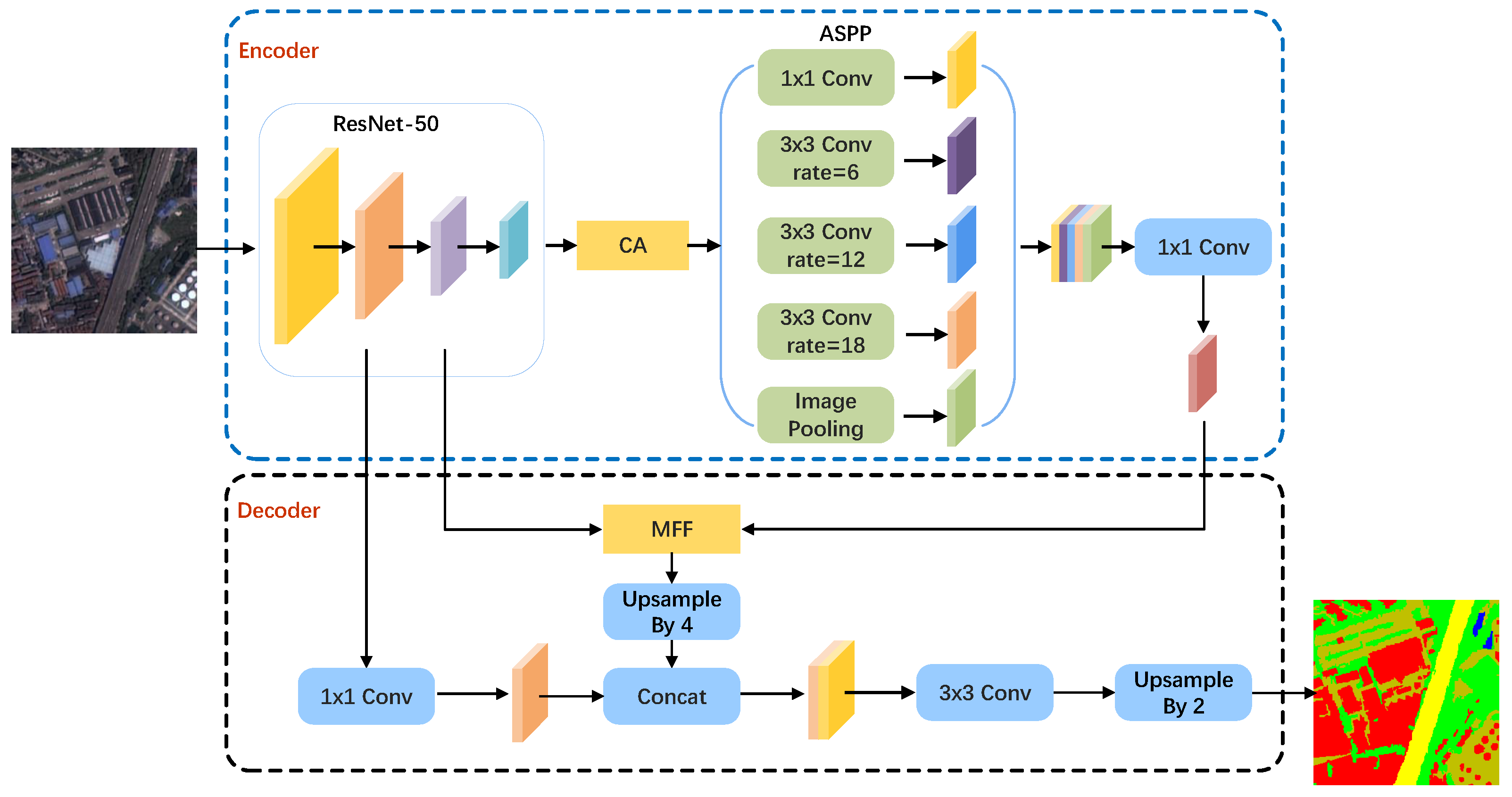
To address the intricate scenarios encountered in object classification for remote sensing images, the proposed RSLC-Deeplab model was designed by combining attention mechanisms and feature fusion methods to automatically extract different ground objects from remote sensing images. To compare the segmentation performance, various segmentation networks including RSLC-Deeplab, DeeplabV3+, U-Net, PSP-NET, and MACU-Net were evaluated on the publicly available WHDLD dataset through experiments. The experimental results showed that RSLC-Deeplab outperformed other comparison networks, effectively enhancing the segmentation ability and reducing the training cost.

2. Methodology

The traditional DeeplabV3+ model was proposed by a team at Google. On the basis of DeeplabV3, DeeplabV3+ has undergone fundamental architectural changes. DeeplabV3+ uses Xception [36] as the backbone network, eliminates the use of fully connected Conditional Random Fields (CRF), and uses DeeplabV3 as the encoder to design a new encoder–decoder structure. In the encoder, a deep convolutional neural network is employed to extract features from the input image. Then, ASPP obtains rich contextual information by utilizing multi-scale atrous convolution and pyramid pooling from the output features of the backbone network. The semantic information features of various scales are integrated, and the fused high-level semantic features with multiple scales are adjusted in terms of channel number and upsampled using bilinear interpolation. In the decoder, the upsampled high-level semantic features are used to restore spatial resolution. During the process of feature map resolution recovery, the low-level features extracted from the backbone network are concatenated with the high-level features. The low-level features possess better perceptual abilities for capturing fine-grained details, such as small objects or edges, resulting in improved accuracy when localizing and segmenting small objects within the image. Finally, four-times bilinear interpolation upsampling is used to generate the final prediction image.

The feature extraction process in the DeeplabV3+ network utilizes the Xception backbone network. The Xception backbone network possesses a substantial amount of layers and parameters, resulting in high model complexity and a slow training speed. Based on improvements made to the original DeeplabV3+ model, RSLC-Deeplab is proposed to enhance the segmentation performance and training efficiency, as shown in Figure 1. The main contributions of the RSLC-Deeplab model proposed in this paper are as follows:

• In the encoder, ResNet-50 is used instead of the original Xception as the feature extraction module, which can capture more refined features.
• After the backbone network, the CA module is introduced to embed positional information into the channel attention mechanism, enabling neural networks to better comprehend input data and improve prediction accuracy.
• In the decoder, we designed an MFF module, which captures and refines low-level spatial features using asymmetric convolution and then fuses them with high-level abstract features to mitigate the influence of background noise and restore the lost detailed information in deep features.

Figure 1. Structure diagram of RSLC-Deeplab.

Figure 1. Structure diagram of RSLC-Deeplab.

2.1. Optimized Feature Extraction Module

In the encoder, the feature extraction network for RSLC-Deeplab is ResNet-50 [37], and

Table 1. ResNet-50 network structure.

Output Size	Network	Output Channel	Module Repetitions
128 × 128	7 × 7, 64	64	1
64 × 64	3 × 3, max pool	64	1
64 × 64	Bottleneck	256	3
32 × 32	Bottleneck	512	4
16 × 16	Bottleneck	1024	6
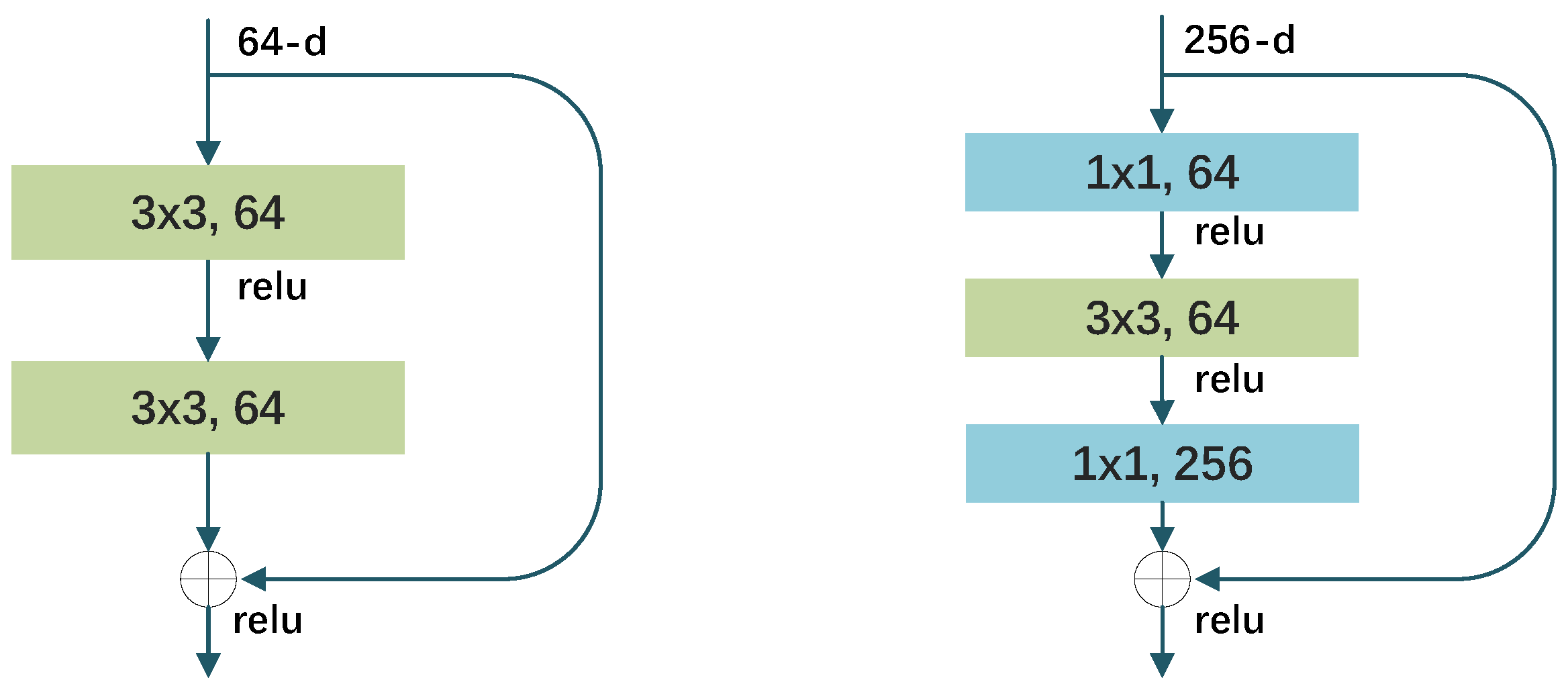
8 × 8	Bottleneck	2048	3

depicts its structure. We know that the depth of a network is crucial for effective feature extraction. Deep convolutional networks utilize an end-to-end multi-layer approach to integrate features at different levels, achieved through the stacking of convolutional layers and downsampling layers. When the network is stacked to a certain depth, gradient vanishing and gradient explosion problems will occur. Data preprocessing and the incorporation of batch normalization (BN) in the network are effective solutions to address these issues. However, as the network depth increases and convergence is achieved, another challenge emerges: the accuracy tends to reach a plateau and subsequently deteriorate rapidly. Therefore, ResNet introduces a residual structure to alleviate the degradation problem of network performance.

Compared to traditional convolutional neural networks, the residual structure can directly pass low-level features to high-level layers through shortcut connections, which enhances the smooth flow of information within the network. This helps the network to better capture details and local features and improves the reusability of features, thereby enhancing the network’s performance. The shortcut connection skips the connection of one or more layers and directly combines its output with the output of the stacked layers. This approach not only avoids introducing additional parameters or computational complexity, but also facilitates gradient propagation and enables feature reuse. The formula is as follows:

$$y=F\left(x\right)+x$$

(1)

where x and y represent the input and output features, respectively, and the function $F\left(x\right)$ represents the residual mapping composed of stacked nonlinear layers. For residual networks with different network depths, there are two different residual structures. The residual structure on the left of Figure 2 is suitable for networks with fewer layers, while the residual structure on the right is more suitable for networks with more layers. In ResNet-50, the $F\left(x\right)$ function of the residual structure is composed of three stacked layers: 1 × 1, 3 × 3, and 1 × 1 convolution. The channel number is first reduced by 1 × 1 convolution, then 3 × 3 convolution is performed, and finally the channel number is restored by 1 × 1 convolution.

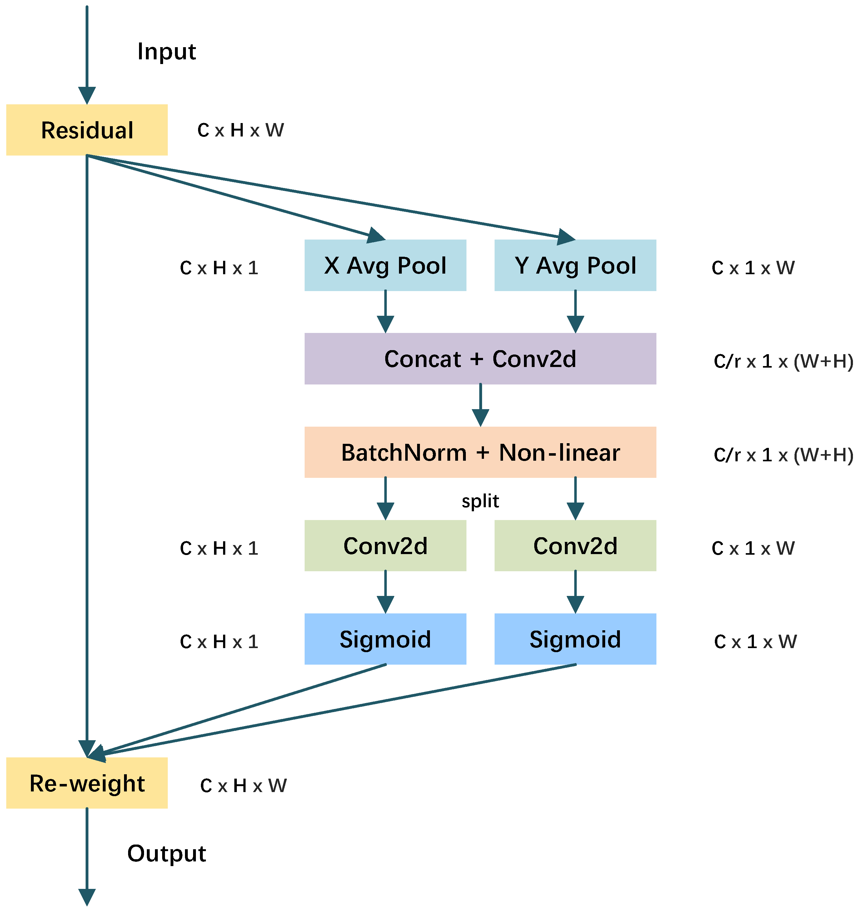
2.2. CA Module

The origin of attention mechanisms can be traced back to studies on human vision, where researchers aimed to develop models of visual selective attention that could simulate the intricate process of human visual perception. It has been empirically established that incorporating attention mechanisms into convolutional neural networks enhances the ability to capture crucial information. The core principle underlying attention mechanisms entails learning the regions of interest in each image via the process of forward propagation and negative feedback, followed by the assignment of appropriate attention weights. In order to effectively capture the relationships between channels, a Coordinate Attention (CA) module is introduced subsequent to the feature extraction network module. The CA module is mainly implemented through two steps: embedding coordinate information and generating coordinate attention. The CA module dynamically adjusts weights to model dependencies between different distances, enabling the model to better capture global information within images. The specific structure is depicted in Figure 3.

Due to the prevalent utilization of global pooling in channel attention mechanisms for the purpose of globally encoding spatial information, there exists a potential risk of losing positional information. In the coordinate information embedding module, for the input feature X, a pooling kernel of dimensions (H,1) and (1,W) is employed to encode each channel along the horizontal and vertical coordinate directions, respectively. By using a pair of one-dimensional features to encode the features of each location into a unique vector, the network can better understand and utilize location information. Consequently, the output of the c-th channel, characterized by a height (h) and width (w), can be expressed as follows:

$$z_c^h\left(h\right)=\frac{1}{W}{\displaystyle \sum _{0\le i\le W}}{x}_c\left(h,i\right)$$

(2)

$$z_c^w\left(w\right)=\frac{1}{H}{\displaystyle \sum _{0\le j\le H}}{x}_c\left(j,w\right)$$

(3)

By combining features along both the horizontal and vertical directions, a set of feature maps that are sensitive to directional information is generated. This pair of transformations helps the attention block gain the ability to apprehend distant correlations within a particular spatial orientation while upholding the integrity of precise positional data in the alternative spatial orientation. Consequently, such operations assist the network in effectively locating desired objects. After performing cascaded operations on the aggregated feature maps, they are further processed using a 1 × 1 convolutional transformation function, F${}_1$, which is expressed as follows:

$$f=\delta \left(F_1\left[z^h,z^w\right]\right)$$

(4)

where $\left[·,·\right]$ denotes the concatenation operation along the horizontal and vertical coordinate directions, $\delta$ denotes the non-linear activation function, and f represents the intermediate feature map that encodes spatial information. Subsequently, f is partitioned into two separate tensors, namely $f^h\in R^{C/r\times H}$ and $f^w\in R^{C/r\times W}$, along the spatial dimension. Here, the variable r specifically denotes the reduction ratio employed to regulate the block size within the SE block. Subsequently, $f^h$ and $f^w$ undergo separate 1 × 1 convolutions, denoted as $F_h$ and $F_w$, respectively, to match the channel dimensions of the input tensor X, as follows:

$$g^h=\sigma \left(F_h\left(f^h\right)\right)$$

(5)

$$g^w=\sigma \left(F_w\left(f^w\right)\right)$$

(6)

where $\sigma$ represents the sigmoid activation function. Then, $g^h$ and $g^w$ are expanded as attention weights, and the final output Y of CA is as follows:

$$y_c\left(i,j\right)=x_c\left(i,j\right)\times g_c^h\left(i\right)\times g_c^w\left(j\right)$$

(7)

2.3. MFF Module

Due to the three downsampling operations in the feature extraction process of the backbone network, the decrease in resolution leads to the loss of spatial information for finer details. In the decoder part of the original DeeplabV3+ network model, the problem of lost segmentation object detail is improved to some extent by directly concatenating the deep features output by the encoder with the shallow features from the backbone network, but it is still not precise enough for segmenting complex objects such as object boundaries and small targets. To further improve segmentation accuracy, a multilevel feature fusion module (MFF) is introduced, as illustrated in Figure 4.

During the process of multilevel feature fusion, the shallow features. $F_1$, obtained from the third downsampling of the backbone network and the deep features, $F_2$, from the encoder output are used as inputs. To fuse the local spatial information in $F_1$ with the global semantic information in $F_2$, asymmetric convolution is utilized to extract features from the shallow features, $F_1$, which are then concatenated and fused with the deep features, $F_2$. By effectively combining shallow and deep features, this method enhances the overall accuracy of the segmentation model.

Compared to normal convolution, asymmetric convolution has a stronger feature representation ability. The weights of the square convolution kernel are typically larger than those of the corners, which can lead to uneven feature refinement. Asymmetric convolution uses three parallel convolutional layers: 3 × 3 convolution, 1 × 3 convolution, and 3 × 1 convolution. The 3 × 3 convolution obtains features from a larger receptive field, while the 1 × 3 and 3 × 1 convolutions can obtain receptive fields in the horizontal and vertical directions, respectively. This allows the network to effectively collect the correlation information of different spatial scales, which is particularly useful for tasks such as semantic segmentation, where capturing detailed spatial information is crucial. Finally, the outcomes of three convolution operations are added to further enrich the spatial features. The formula for asymmetric convolution is

$$x_i^{\prime }=F_{3\times 3}\left(x_{i-1}\right)+F_{1\times 3}\left(x_{i-1}\right)+F_{3\times 1}\left(x_{i-1}\right)$$

(8)

$$x_i=\sigma \left(\gamma \frac{x_i^{\prime }-\mu \left(x_i^{\prime }\right)}{\sqrt{\upsilon \left(x_i^{\prime }\right)+{\epsilon }_i}}+\beta \right)$$

(9)

where $x_{i-1}$ is the input feature, $x_i$ is the output feature, $\upsilon$ is the expected value of the input, ${\epsilon }_i$ is a small constant to ensure numerical stability, $\gamma$ and $\beta$ represent the two trainable parameters of the BN layer, and $\sigma$ represents the ReLU activation function.

3. Experiment

3.1. Experimental Data

The dataset used in this study was the publicly available remote sensing image dataset WHDLD (https://sites.google.com/view/zhouwx/dataset#h.p_hQS2jYeaFpV0 (accessed on 27 August 2023)), which was released by Wuhan University. It consists of 4940 images captured by GF-1 and ZY-3, with each image being an RGB image and having a resolution of 256 × 256 pixels. The pixel-level annotations of the dataset include six classes: water, vegetation, building, road, bare soil, and pavement.

According to the statistics, the WHDLD dataset exhibits an issue of imbalanced pixel distribution among different classes. Therefore, we employed augmentation techniques, including horizontal flipping, vertical flipping, 90-degree rotation, 180-degree rotation, 270-degree rotation, and brightness adjustment, to enhance classes with a lower pixel count, such as road, bare soil, and building. The dataset was expanded to a total of 6700 images, and the augmented samples are illustrated in Figure 5. The dataset was divided into training, validation, and testing sets in an 8:1:1 ratio. The example images and labels of the WHDLD dataset are shown in Figure 6.

3.2. Implementation Details

Experimental verification was conducted on the proposed algorithm, and the configuration parameters of the experimental platform are shown in

Table 2. Information about the experimental platform.

Experimental Environment	Configuration Information
Operating system	Windows 10
CPU	Intel(R) Core(TM) i7-11700F
GPU	NVIDIA GeForce RTX 3060
Cuda	Cuda 11.3
Framework	Pytorch 1.10.0

. The transfer learning approach was used in the experiment, where the pre-trained model weights of the backbone network were loaded before training to accelerate the model’s convergence. The SGD optimizer was selected for network gradient updates. The initial learning rate of the experiment was 0.007, the momentum coefficient was 0.9, the batch size was 12, and the training epoch was 200.

The experiment utilized the cross-entropy loss function to quantify the disparity between the model’s predictions and the actual results, a technique that is well-suited for classification tasks. It has the benefits of being easy to compute and optimize and usually produces good results in training neural networks, so it can effectively guide a model to learn the task objectives. Since the pixels in the input image of this experiment had six categories, the experiments used the following multi-category cross-entropy loss function:

$$Loss=-\frac{1}{N}{\displaystyle \sum _{i=1}^N}{\displaystyle \sum _{k=1}^K}{y}_{i,k}log{p}_{i,k}$$

(10)

where $y_{i,k}$ is the true class of the i-th sample, taking a value of 1 if it belongs to the k-th class and 0 otherwise, with N samples and K classes in total. Meanwhile, $p_{i,k}$ is the probability of the i-th sample being predicted as the k-th class.

3.3. Evaluation Metrics

After the model was trained, the trained weights were used for testing with the test set. The accuracy of classification was analyzed using a confusion matrix, as shown in

Table 3. Confusion matrix.

		Predicted Label
		True	False
GT data	True	TP (true positive)	FN (false negative)
	False	FP (false positive)	TN (true negative)

. TP (true positive) represents correctly classified positive samples, while FP (false positive) represents incorrectly classified negative samples. Conversely, FN (false negative) represents incorrectly classified positive samples, and TN (true negative) represents correctly classified negative samples.

The experiment employed key metrics such as pixel accuracy (PA), mean pixel accuracy (mPA), and mean intersection over union (mIoU) were used in the experiment to measure the differences between the predicted and ground-truth images. The formulas are as follows:

$$PA=\frac{{\sum }_{i=0}^n{p}_{ii}}{{\sum }_{i=0}^n{\sum }_{j=0}^n{p}_{ij}}$$

(11)

$$mPA=\frac{1}{n}{\displaystyle \sum _{i=0}^n}\frac{p_{ii}}{{\sum }_{i=0}^n{\sum }_{j=0}^n{p}_{ij}}$$

(12)

$$mIoU=\frac{1}{n}{\displaystyle \sum _{k=1}^n}\frac{T{P}_k}{T{P}_k+F{P}_k+F{N}_k}$$

(13)

where n is the number of classes including the background class, $p_{ii}$ is the count of pixels of class i predicted as class i, and $p_{ij}$ is the count of pixels of class i predicted as class j.

3.4. Comparative Experiment of Different Backbone Networks

A backbone network is a pre-trained model utilized for extracting image features and providing enhanced feature representation for subsequent semantic segmentation tasks. To select an appropriate backbone network as the feature extraction network for the model, five comparative experiments were conducted using different backbone networks within the original DeeplabV3+ [30] network architecture.

Table 4. Comparative experimental results of different backbone networks.

Method	Backbone	mIoU (%)	Parameters (M)	Flops (G)	Model Size (M)
Scheme 1	Xception	68.50	54.71	41.72	209.70
Scheme 2	MobileNetV2	67.44	5.81	13.23	22.44
Scheme 3	EfficientNetV2	69.68	31.25	100.10	120.12
Scheme 4	ResNet-101	70.81	59.33	76.29	226.98
Scheme 5	ResNet-50	70.48	40.34	66.54	154.23

presents the experimental data.

In Table 4, Scheme 5 used ResNet-50 [37] as the backbone network, with an mIoU of 70.48%, a parameter count of 40.34 M, a computational cost of 66.54 G, and a model size of 154.23 M. Scheme 1 used Xception [36] as the backbone network, and Scheme 5 had an mIoU increase of 1.98% compared to Scheme 1, with a significantly smaller parameter count and model size. Scheme 2 used MobileNetv2 [38] as the backbone network, and although the parameter count and model size were greatly reduced, its mIoU was 3.04% lower than that of Scheme 5, indicating insufficient segmentation accuracy. Scheme 3 used EfficientNetV2 [39] as the backbone network, and its mIoU was 0.80% lower than that of Scheme 5, with a smaller parameter count but a much larger computational cost than Scheme 5. Scheme 4 used ResNet-101 as the backbone network, and although its mIoU was 0.33% higher than that of Scheme 5, its parameter count and model size were much larger than those of Scheme 5. After a comprehensive analysis, ResNet-50 was chosen as the feature extraction module of this task, not only improving the semantic segmentation accuracy, but also optimizing the model complexity.

3.5. Ablation Experiment

To validate the efficacy of the ResNet-50 network, the CA module, and the MFF module, a set of experiments were designed by gradually introducing the ResNet-50 backbone network, CA attention module, and MFF module. Table 5 presents the experimental data.

Scheme 1: The original Deeplabv3+ network, which employed Xception as the feature extraction network, was used as the baseline.

Scheme 2: ResNet-50 was used as the feature extraction network to replace Xception in Scheme 1.

Scheme 3: The CA module was introduced on the basis of Scheme 2, which enhanced the feature representation generated by the network, enabling neural networks to better comprehend input data and improve prediction accuracy.

Scheme 4: The MFF module was introduced on the basis of Scheme 2, which captured and refined low-level spatial features using asymmetric convolution and then fused them with high-level abstract features to improve segmentation accuracy.

Scheme 5: On the basis of Scheme 2, both the CA module and the MFF module were introduced simultaneously.

Table 5. Results of ablation experiments on different modules.

Method	Backbone	CA	MFF	PA (%)	mPA (%)	mIoU (%)
Scheme 1	Xception			80.38	80.47	68.50
Scheme 2	ResNet-50			81.92	81.89	70.48
Scheme 3	ResNet-50	✓		82.63	82.45	71.67
Scheme 4	ResNet-50		✓	82.78	82.86	71.73
Scheme 5	ResNet-50	✓	✓	83.49	83.72	72.63

Table 5. Results of ablation experiments on different modules.

Method	Backbone	CA	MFF	PA (%)	mPA (%)	mIoU (%)
Scheme 1	Xception			80.38	80.47	68.50
Scheme 2	ResNet-50			81.92	81.89	70.48
Scheme 3	ResNet-50	✓		82.63	82.45	71.67
Scheme 4	ResNet-50		✓	82.78	82.86	71.73
Scheme 5	ResNet-50	✓	✓	83.49	83.72	72.63

As shown in Table 5, the PA, mPA, and mIoU values of Scheme 1 were 80.38%, 80.47%, and 68.50%, respectively. Scheme 2 utilized ResNet-50 as the feature extraction network, and its PA, mPA, and mIoU values were 81.92%, 81.89%, and 70.48%, respectively. Compared to Scheme 1, the PA, mPA, and mIoU values improved by 1.54%, 1.42%, and 1.98%, respectively. Based on Scheme 2, Scheme 3 introduced a CA module, yielding PA, mPA, and mIoU values of 82.63%, 82.45%, and 71.67%, respectively. Compared to Scheme 2, the PA, mPA, and mIoU values improved by 0.71%, 0.56%, and 1.19%, respectively. Scheme 4 introduced an MFF module to further restore the edge details of the segmentation image by fusing low-level and high-level features, with PA, mPA, and mIoU values of 82.78%, 82.86%, and 71.73%, respectively. Compared to Scheme 2, the PA, mPA, and mIoU values improved by 0.86%, 0.97%, and 1.25%, respectively. Scheme 5 simultaneously introduced both the CA and MFF modules, with PA, mPA, and mIoU values of 83.49%, 83.72%, and 72.63%, respectively. Compared to the original DeepLabV3+ model, the PA, mPA, and mIoU values improved by 3.11%, 3.25%, and 4.13%, respectively. The experimental results indicate that RSLC-Deeplab exhibited impressive segmentation performance.

The experiments used SGD as the optimizer, which updated the model parameters by computing the gradients of each training sample and gradually reducing the model’s loss function. The performance variation of different approaches at different stages is depicted in Figure 7. Using ResNet-50 as the backbone network, the mIoU value increased rapidly at the beginning and then tended to converge, with a significant improvement in mIoU values. After gradually introducing the CA and MFF modules, the model had the ability to fit the training data faster and achieve better segmentation results, indicating that the design and training methods of the model were effective. The training and validation loss values of the RSLC-Deeplab algorithm on the WHDLD dataset are shown in Figure 8. During the initial stages of the experiment, both the training and validation losses decreased rapidly; then, the decreasing trend slowed down after a certain number of iterations, before finally tending to converge.

3.6. Comparative Experiment of Different Methods

We conducted comparative experiments between RSLC-Deeplab and other models, including DeeplabV3+ [30], U-Net [21], PSP-Net [25], and MACU-Net [23], on the WHDLD dataset to verify the segmentation performance of RSLC-Deeplab. The experimental results of different network models are shown in

Table 6. Comparative experimental results of different segmentation methods.

Method	PA (%)	mPA (%)	mIoU (%)
DeeplabV3+	80.38	80.47	68.50
U-Net	72.73	75.35	63.31
PSPNet	69.54	72.32	60.36
MACU-Net	77.93	79.81	67.64
RSLC-Deeplab	83.49	83.72	72.63

. The results obtained in this study reveal that RSLC-Deeplab outperformed the other networks. The PA, mPA, and mIoU of the proposed method were 83.49%, 83.72%, and 72.63%, respectively, which were 3.11%, 3.25%, and 4.13% higher than those of DeeplabV3+ and 5.56%, 3.91%, and 4.99% higher than those of MACU-Net.

At the same time, the remote sensing image segmentation results produced by RSLC-Deeplab and the comparative methods are presented in Figure 9. As illustrated in the diagram, PSPNet, and U-Net could roughly segment large-scale ground objects, but their segmentation ability for small-scale targets and object edges was poor, resulting in many misclassifications and omissions. MACU-Net demonstrated a certain improvement in segmentation ability compared to U-Net, but there were still problems of misclassification and omission in categories such as buildings, vegetation, and water bodies. DeeplabV3+ showed a greater improvement in segmentation ability than the classical semantic segmentation methods, but it still could not accurately segment the edge feature information of small-scale categories such as buildings, water bodies, and bare soil. The proposed RSLC-Deeplab improved the segmentation accuracy of small-scale landform targets, and the edge segmentation of categories such as buildings, roads, and vegetation was clearer, without many misclassifications and omissions. The experiment proved that RSLC-Deeplab captured more detailed features and improved the segmentation accuracy of small targets.

This study also took into account the metrics of parameter size and training time. The parameter size and training time per epoch of the compared methods are presented in

Table 7. Comparison of training time and parameter size of different methods.

Method	Training Time (s)/Epoch	Parameters (M)
PSPNet	181	48.97
U-Net	217	34.53
MACU-Net	266	5.17
DeeplabV3+	304	54.71
RSLC-Deeplab	239	47.62

. The parameter size of RSLC-Deeplab was 47.62M, and the training time was 239s. The experimental results demonstrated a significant reduction in both training time and parameter size for RSLC-Deeplab compared to the original DeeplabV3+ network. MACU-Net showed a smaller parameter size, but it had a more complex model structure, resulting in a longer training time. RSLC-Deeplab used ResNet-50 as the feature extraction network, which significantly reduced the model’s parameter size and computation amount.

4. Conclusions

This paper proposed RSLC-Deeplab for high-resolution remote sensing image semantic segmentation. Firstly, ResNet-50 was used as the backbone network, which had a stronger feature extraction ability while reducing the parameter size and computation amount, providing better feature representation for subsequent segmentation. Secondly, the CA mechanism was used after the feature extraction module to embed positional information into the channel attention mechanism, enabling neural networks to better comprehend input data and improve prediction accuracy. Finally, a multi-level feature fusion (MFF) module based on asymmetric convolution was proposed, which captured and refined low-level spatial features using asymmetric convolution and then fused them with high-level abstract features. The MFF module effectively eliminated background noise during feature extraction and improved the clarity of segmentation boundaries.

On the WHDLD remote sensing image dataset, our model achieved an mIoU of 72.63% and an mPA of 83.72%, which significantly improved issues such as mis-segmentation and edge detail blurring. Compared with other methods, our model obtained more accurate segmentation results. On this basis, we will further optimize the segmentation accuracy of the model for categories with a low segmentation accuracy and continue to study how to suppress the impact of interfering factors such as background noise and shadows in the image to enhance the model’s overall segmentation capability.

References

1. Kemker, R.; Salvaggio, C.; Kanan, C. Algorithms for semantic segmentation of multispectral remote sensing imagery using deep learning. ISPRS J. Photogramm. Remote Sens. 2018, 145, 60–77. [Google Scholar] [CrossRef]
2. Yao, H.; Qin, R.; Chen, X. Unmanned aerial vehicle for remote sensing applications—A review. Remote Sens. 2019, 11, 1443. [Google Scholar] [CrossRef]
3. Zhao, Q.; Liu, J.; Li, Y.; Zhang, H. Semantic segmentation with attention mechanism for remote sensing images. IEEE Trans. Geosci. Remote Sens. 2021, 60, 1–13. [Google Scholar] [CrossRef]
4. Zhang, Q.; Yang, G.; Zhang, G. Collaborative network for super-resolution and semantic segmentation of remote sensing images. IEEE Trans. Geosci. Remote Sens. 2021, 60, 1–12. [Google Scholar] [CrossRef]
5. Yuan, Y.; Chen, X.; Wang, J. Object-contextual representations for semantic segmentation. In Proceedings of the Computer Vision–ECCV 2020: 16th European Conference, Glasgow, UK, 23–28 August 2020; Proceedings, Part VI 16. Springer: Berlin/Heidelberg, Germany, 2020; pp. 173–190. [Google Scholar]
6. Cuevas, E.; Zaldivar, D.; Pérez-Cisneros, M. A novel multi-threshold segmentation approach based on differential evolution optimization. Expert Syst. Appl. 2010, 37, 5265–5271. [Google Scholar] [CrossRef]
7. Chen, J.; Li, J.; Pan, D.; Zhu, Q.; Mao, Z. Edge-guided multiscale segmentation of satellite multispectral imagery. IEEE Trans. Geosci. Remote Sens. 2012, 50, 4513–4520. [Google Scholar] [CrossRef]
8. Byun, Y.; Kim, D.; Lee, J.; Kim, Y. A framework for the segmentation of high-resolution satellite imagery using modified seeded-region growing and region merging. Int. J. Remote Sens. 2011, 32, 4589–4609. [Google Scholar] [CrossRef]
9. Csillik, O. Fast segmentation and classification of very high resolution remote sensing data using SLIC superpixels. Remote Sens. 2017, 9, 243. [Google Scholar] [CrossRef]
10. Sziranyi, T.; Shadaydeh, M. Segmentation of remote sensing images using similarity-measure-based fusion-MRF model. IEEE Geosci. Remote Sens. Lett. 2014, 11, 1544–1548. [Google Scholar] [CrossRef]
11. Zhang, X.; Xiao, P.; Feng, X.; Wang, J.; Wang, Z. Hybrid region merging method for segmentation of high-resolution remote sensing images. ISPRS J. Photogramm. Remote Sens. 2014, 98, 19–28. [Google Scholar] [CrossRef]
12. Mitra, P.; Shankar, B.U.; Pal, S.K. Segmentation of multispectral remote sensing images using active support vector machines. Pattern Recognit. Lett. 2004, 25, 1067–1074. [Google Scholar] [CrossRef]
13. Bruzzone, L.; Chi, M.; Marconcini, M. A novel transductive SVM for semisupervised classification of remote-sensing images. IEEE Trans. Geosci. Remote. Sens. 2006, 44, 3363–3373. [Google Scholar] [CrossRef]
14. Pal, M. Random forest classifier for remote sensing classification. Int. J. Remote Sens. 2005, 26, 217–222. [Google Scholar] [CrossRef]
15. Mellor, A.; Haywood, A.; Stone, C.; Jones, S. The performance of random forests in an operational setting for large area sclerophyll forest classification. Remote Sens. 2013, 5, 2838–2856. [Google Scholar] [CrossRef]
16. Li, R.; Zheng, S.; Zhang, C.; Duan, C.; Wang, L.; Atkinson, P.M. ABCNet: Attentive bilateral contextual network for efficient semantic segmentation of Fine-Resolution remotely sensed imagery. ISPRS J. Photogramm. Remote Sens. 2021, 181, 84–98. [Google Scholar] [CrossRef]
17. Yang, X.; Li, S.; Chen, Z.; Chanussot, J.; Jia, X.; Zhang, B.; Li, B.; Chen, P. An attention-fused network for semantic segmentation of very-high-resolution remote sensing imagery. ISPRS J. Photogramm. Remote Sens. 2021, 177, 238–262. [Google Scholar] [CrossRef]
18. Long, J.; Shelhamer, E.; Darrell, T. Fully convolutional networks for semantic segmentation. In Proceedings of the IEEE Conference on Computer Vision and Pattern Recognition, Boston, MA, USA, 7–15 June 2015; pp. 3431–3440. [Google Scholar]
19. Zhong, Z.; Li, J.; Cui, W.; Jiang, H. Fully convolutional networks for building and road extraction: Preliminary results. In Proceedings of the 2016 IEEE International Geoscience and Remote Sensing Symposium (IGARSS), Beijing, China, 10–15 July 2016; pp. 1591–1594. [Google Scholar]
20. Badrinarayanan, V.; Kendall, A.; Cipolla, R. Segnet: A deep convolutional encoder-decoder architecture for image segmentation. IEEE Trans. Pattern Anal. Mach. Intell. 2017, 39, 2481–2495. [Google Scholar] [CrossRef]
21. Ronneberger, O.; Fischer, P.; Brox, T. U-net: Convolutional networks for biomedical image segmentation. In Proceedings of the Medical Image Computing and Computer-Assisted Intervention–MICCAI 2015: 18th International Conference, Munich, Germany, 5–9 October 2015; Proceedings, Part III 18. Springer: Berlin/Heidelberg, Germany, 2015; pp. 234–241. [Google Scholar]
22. Cao, K.; Zhang, X. An improved res-unet model for tree species classification using airborne high-resolution images. Remote Sens. 2020, 12, 1128. [Google Scholar] [CrossRef]
23. Li, R.; Zheng, S.; Duan, C.; Su, J.; Zhang, C. Multistage attention ResU-Net for semantic segmentation of fine-resolution remote sensing images. IEEE Geosci. Remote Sens. Lett. 2021, 19, 1–5. [Google Scholar] [CrossRef]
24. Yu, F.; Koltun, V. Multi-scale context aggregation by dilated convolutions. arXiv 2015, arXiv:1511.07122. [Google Scholar]
25. Zhao, H.; Shi, J.; Qi, X.; Wang, X.; Jia, J. Pyramid scene parsing network. In Proceedings of the IEEE Conference on Computer Vision and Pattern Recognition, Honolulu, HI, USA, 21–26 July 2017; pp. 2881–2890. [Google Scholar]
26. Chen, L.C.; Papandreou, G.; Kokkinos, I.; Murphy, K.; Yuille, A.L. Semantic image segmentation with deep convolutional nets and fully connected crfs. arXiv 2014, arXiv:1412.7062. [Google Scholar]
27. Simonyan, K.; Zisserman, A. Very deep convolutional networks for large-scale image recognition. arXiv 2014, arXiv:1409.1556. [Google Scholar]
28. Chen, L.C.; Papandreou, G.; Kokkinos, I.; Murphy, K.; Yuille, A.L. Deeplab: Semantic image segmentation with deep convolutional nets, atrous convolution, and fully connected crfs. IEEE Trans. Pattern Anal. Mach. Intell. 2017, 40, 834–848. [Google Scholar] [CrossRef]
29. Chen, L.C.; Papandreou, G.; Schroff, F.; Adam, H. Rethinking atrous convolution for semantic image segmentation. arXiv 2017, arXiv:1706.05587. [Google Scholar]
30. Chen, L.C.; Zhu, Y.; Papandreou, G.; Schroff, F.; Adam, H. Encoder-decoder with atrous separable convolution for semantic image segmentation. In Proceedings of the European Conference on Computer Vision (ECCV), Munich, Germany, 8–14 September 2018; pp. 801–818. [Google Scholar]
31. Wang, Z.; Wang, J.; Yang, K.; Wang, L.; Su, F.; Chen, X. Semantic segmentation of high-resolution remote sensing images based on a class feature attention mechanism fused with Deeplabv3+. Comput. Geosci. 2022, 158, 104969. [Google Scholar] [CrossRef]
32. Hu, J.; Shen, L.; Sun, G. Squeeze-and-excitation networks. In Proceedings of the IEEE Conference on Computer Vision and Pattern Recognition, Salt Lake City, UT, USA, 18–23 June 2018; pp. 7132–7141. [Google Scholar]
33. Wang, Q.; Wu, B.; Zhu, P.; Li, P.; Zuo, W.; Hu, Q. ECA-Net: Efficient channel attention for deep convolutional neural networks. In Proceedings of the IEEE/CVF Conference on Computer Vision and Pattern Recognition, Seattle, WA, USA, 13–19 June 2020; pp. 11534–11542. [Google Scholar]
34. Woo, S.; Park, J.; Lee, J.Y.; Kweon, I.S. Cbam: Convolutional block attention module. In Proceedings of the European Conference on Computer Vision (ECCV), Munich, Germany, 8–14 September 2018; pp. 3–19. [Google Scholar]
35. Hou, Q.; Zhou, D.; Feng, J. Coordinate attention for efficient mobile network design. In Proceedings of the IEEE/CVF Conference on Computer Vision and Pattern Recognition, Nashville, TN, USA, 20–25 June 2021; pp. 13713–13722. [Google Scholar]
36. Chollet, F. Xception: Deep learning with depthwise separable convolutions. In Proceedings of the IEEE Conference on Computer Vision and Pattern Recognition, Honolulu, HI, USA, 21–26 July 2017; pp. 1251–1258. [Google Scholar]
37. He, K.; Zhang, X.; Ren, S.; Sun, J. Deep residual learning for image recognition. In Proceedings of the IEEE Conference on Computer Vision and Pattern Recognition, Las Vegas, NV, USA, 26–30 June 2015; pp. 770–778. [Google Scholar]
38. Sandler, M.; Howard, A.; Zhu, M.; Zhmoginov, A.; Chen, L.C. Mobilenetv2: Inverted residuals and linear bottlenecks. In Proceedings of the IEEE Conference on Computer Vision and Pattern Recognition, Salt Lake City, UT, USA, 18–23 June 2018; pp. 4510–4520. [Google Scholar]
39. Tan, M.; Le, Q. Efficientnetv2: Smaller models and faster training. In Proceedings of the International Conference on Machine Learning, Virtual Event, 18–24 July 2021; pp. 10096–10106. [Google Scholar]
Figure 2. A deeper residual structure. Left: ResNet-34 building block. Right: “Bottleneck” building block for ResNet-50/101/152.
Electronics 12 03653 g002
Figure 3. The CA module.
Electronics 12 03653 g003
Figure 4. Structure of the MFF.
Electronics 12 03653 g004
Figure 5. The augmented samples.
Electronics 12 03653 g005
Figure 6. Dataset samples.
Electronics 12 03653 g006
Figure 7. The mIoU values of different schemes in ablation experiments.
Electronics 12 03653 g007
Figure 8. The loss values of RSLC-Deeplab on the training and validation sets.
Electronics 12 03653 g008
Figure 9. Diagram of the segmentation effect of different methods.
Electronics 12 03653 g009