Article

Diffuse Reflection Effects in Visible Light Positioning: Analysis, Modeling, and Evaluation

1
The State Key Laboratory of Deep Coal Mine Mining Response and Disaster Prevention and Control, Anhui University of Science and Technology, Huainan 232002, China
2
College of Electronic Information, Wuhan University, Wuhan 430072, China
3
The State Key Laboratory of Engineering in Surveying, Mapping and Remote Sensing (LIESMARS), Wuhan University, Wuhan 430072, China
*
Author to whom correspondence should be addressed.
Electronics 2023, 12(17), 3646; https://doi.org/10.3390/electronics12173646
Submission received: 14 July 2023 / Revised: 8 August 2023 / Accepted: 10 August 2023 / Published: 29 August 2023
(This article belongs to the Special Issue Recent Research in Positioning and Activity Recognition Systems)

Abstract

:
Currently, the Global Positioning System (GPS) is widely used, but its signal is attenuated by factors such as trees, walls, and ceilings, which severely degrade its positioning accuracy. To fill the gap, various indoor positioning techniques have attracted increasing attention in recent years. Visible light positioning (VLP) is a promising scheme for indoor positioning due to its high precision, high security, and low energy consumption; however, ubiquitous diffuse reflection affects the accuracy and robustness of VLP. During our testing, we found that diffuse reflection could increase the error in RSS values by 20~30%, severely affecting VLP accuracy; however, diffuse reflection is inevitable in real positioning environments. To solve this problem, this paper first establishes a wall diffuse reflection model and then implements a visible light positioning system based on an Internet of Things platform. Finally, this paper uses the system to verify the effectiveness of the diffuse reflection model. The experiments show that the proposed model effectively improves positioning accuracy by 36.7~61.3%.

1. Introduction

The Global Positioning System (GPS) is a widely used positioning technology [1], but it suffers from significant attenuation in challenging environments due to various interference factors such as trees, walls, and ceilings. According to Kerem Özsoy [2], GPS indoor localization can reach an accuracy of only approximately 7 m with the help of power amplifiers under various types of interference. This is insufficient to provide adequate services in the current complex indoor positioning scenarios. However, as urbanization progresses, complex and tall structures increasingly occupy people’s living environments, necessitating higher-precision positioning technologies when addressing the environment [3].
Currently, the main research areas for indoor positioning technology include wireless fidelity (wi-fi) [4], Bluetooth [5], Zigbee [6], radio frequency identification (RFID), infrared, ultrasonic, and visible light [7], optical camera communication (OCC) [8], light detection and ranging (Lidar) [9], and ultra-wideband (UWB) [10]. Wi-fi, Bluetooth, and Zigbee can achieve only limited positioning accuracy. While infrared, ultrasonic, and UWB can provide high-precision localization, they involve high construction costs. LED lights, as energy-efficient and environmentally friendly lighting sources, have become increasingly popular in people’s daily lives. In addition to being more accurate than traditional wireless positioning techniques, they have many advantages, such as low energy consumption, small multipath effects, environmental friendliness, harmlessness to humans, and long service life [11]. Although the construction cost of replacing incandescent bulbs with LED lights indoors is currently high, the maintenance cost of LED lights is low, and the trend is toward more widespread use in future lighting scenarios. The signal reception devices for LED mainly include photodiodes (PDs) and cameras. Although the camera can achieve higher accuracy, it requires higher resolution and a wider field of view, and the computation is more complex. Therefore, this article focuses on simple and efficient PD-based visible light positioning. In recent years, many VLP positioning algorithms based on PD have been proposed and experimentally verified [12], with an average positioning accuracy of centimeters.
Angle of arrival (AOA) [13] and time difference of arrival (TDOA) [14] localization systems exhibit good stability but are complex and tedious to implement, with strict requirements for equipment conditions. Received signal strength (RSS)-based localization has lower complexity and better feasibility with higher accuracy, despite poorer resistance to interference and instability in localization. Reliable anti-noise and anti-interference solutions would make localization systems more suitable for practical applications. Therefore, a visible light localization system based on RSS is constructed, utilizing the latest IoT development chip, ESP32, to address the issues of complexity, sidelobe effects, and frequency instability in current visible light experimental equipment, resulting in a stable, concise, small, and user-friendly experimental setup.
Moreover, the diffuse reflection of objects is unavoidable in all application environments. The complexity of wall geometry and reflection models in reality, along with the significant impact of diffuse reflection on RSS values, makes wall diffuse reflection one of the most challenging interferences to resolve. Based on our own experimental results, the localization accuracy without the wall surface diffuse reflection is 3.04 cm, while with the wall surface diffuse reflection it is 14.73 cm. The introduction of the wall surface diffuse reflection leads to an increase of approximately 3 to 4 times in the localization error.
Nazmi A. Mohammed [15] also stated: “Diffuse reflection had a great impact on the localization error. For example, at the worst operating coordinates, the localization error was estimated to be 2 cm in the case of LOS, whereas it increased to 1.52 m in the case that included the effect of multipath propagation under the following specifications: a transmitted LED power of 1 W, 60° half-power transmitting angle, Rx with 70° FOV, 400 MHz noise BW, and walls with a reflectivity of 0.8”. Currently, there are some articles that have proposed solutions at the theoretical and methodological levels [15,16,17,18], but there are very few researchers who have addressed this problem in real-world scenarios.
To solve this problem, this paper models the impact of single-sided wall diffuse reflection on RSS values using the Lambertian model, and validates its effectiveness in actual localization. Therefore, the main contributions of this paper are summarized as follows:
  • Building a low-cost, stable, and strongly sidelobe-interference-resistant visible light positioning system;
  • Establishing a model for wall diffuse reflection and validating its effectiveness in practical VLP system.

2. Principle of the Proposed VLP System

Figure 1 illustrates the flow chart of the proposed visible light system, in which the LED at the transmitting end is modulated at different frequencies, and after spatial transmission, all LED signals are received by the PD and different LED signal strengths are identified and extracted through FFT. The signal strength is converted to the corresponding distance by the Lambertian model and the position is finally solved through the least squares method.
Indoor visible light transmission links can be distinguished in two aspects: whether the transmitter and receiver have directionality and whether there are obstacles between them. Therefore, it is divided into a line-of-sight (LOS) transmission link and non-line-of-sight (NLOS) transmission link. The LOS transmission link is preferred as the channel is not affected by the multipath.
We use RSS signal localization, which is based on the relationship between the LOS optical intensity and the position. This is an effective link in our optical localization process. Both the LED and PD channel models follow the Lambertian Emission law, which states that the radiation intensity in all directions after the surface reflection of incident light is completely diffuse is the same. The diffuse light intensity is proportional to the cosine of the incident angle and independent of the reflection direction. The received optical power by the PD is shown in Equation (1).
P i ϕ , φ = m + 1 A R P T i 2 π T s φ g φ cos m i ϕ cos M φ d i 2
where d i is the distance between the i t h LED and the receiver, A R is the effective area of the PD at the receiver, P T i is the optical power of the i t h LED source, ϕ is the angle of irradiance, φ is the angle of incidence at the receiver, T s φ is the gain of an optical filter, and g φ is the gain of an optical concentrator placed in front of the sensor [19]. Generally speaking, when there is no lens or filter in front of the PD, T s φ = g φ = 1 . M and m i represent Lambertian orders of the detector and LED chip, respectively. They can be given by:
M = l n 2 l n ( c o s ( φ ( 1 / 2 ) ) ) m i = l n 2 l n ( c o s ( ϕ ( 1 / 2 ) ) )
In order to analyze the relationship between the optical channel gain and the position information of the PD, we simplified the optical channel gain model. Specifically, we assumed that the LED and PD were placed horizontally; consequently, the incidence angle was equal to the radiation angle. The cosine function of the incidence angle satisfies the following equation:
cos ϕ = cos φ = h d
h represents the vertical height between the lamp and PD. d still represents the distance between the LED and the receiver. Therefore, the Lambertian formula can be simplified to:
P L O S i ( ϕ , φ ) = m i + 1 A R P T i 2 π 1 d 2 h d m i + M
Thus, the received signal strength (RSS) value for the line-of-sight (LOS) link is expressed as:
R S S L O S i = a i · d b i a i = m i + 1 A R P T i 2 π h m i + M b i = ( m i + M + 2 )
However, in practical situations, the impact of NLOS and environmental noise on visible light cannot be ignored. Among them, the impact of wall reflection is particularly severe.
According to the light reflection model, when the light beam emitted by the LED light source irradiates the wall, it will be scattered, resulting in diffuse reflected light. The intensity of the diffuse reflected light in different directions is proportional to the cosine of the incidence angle, and it is independent of the reflection direction. This behavior follows the Lambertian radiation law.
The process of wall diffuse reflection can be divided into two steps [20]. First, the LED irradiates the wall, and then the wall diffuse reflection serves as a new light source. Finally, the diffuse reflected light is received by the photodetector (PD).
To calculate the overall DC gain, we need to consider the contributions from both the LED light source and the wall diffuse reflection. The intensity of the diffuse reflected light depends on the incident angle of the light beam on the wall, and is independent of the reflection direction.
Finally, the overall DC gain of diffuse reflection can be described as:
P W a l l i = { W a l l A R Δ A R W m i + 1 P T i 2 π 2 d 1 i 2 d 2 i 2 cos m i ϕ 1 c o s φ 1 c o s ϕ 2 c o s φ 2 T s φ 2 0 φ 2 φ F O V 0 φ 2 > φ F O V
In Equation (6), as shown in Figure 2, it can be seen that the geometry is similar to the line-of-sight (LOS) scenario, with two main differences. First, an additional term of Δ A is introduced, which represents the infinitesimal integration area of the effective wall. Second, a term of R W is included, which represents the coefficient of the wall surface diffuse reflection. ϕ 1 is the light source emission angle, φ 1 is the wall reception angle, ϕ 2 is the wall diffuse emission angle, and φ 2 is the PD reception angle. Similarly to Equation (1), T s φ 2 can be thought of as equal to 1.
We can consider Equation (6) in more depth. A R , R W , and P T i in the equation can be considered as constants under the condition that the LED, wall, and PD are constants. m i can be calculated from b i of Equation (5), which is also constant for a constant single LED. So, the constant parts will be generalized to K i . However, for the four variables cos ϕ 1 , cos φ 1 , cos ϕ 2 , cos φ 2 , d 1 i , and d 2 i , we set up the red coordinate system in Figure 2, assuming that the position of the LED is P L E D X 1 i , Y 1 i , Z 1 i , the current position of the microelement Δ A of the wall is P W a l l X 2 , Y 2 , Z 2 , and the position of the PD is P P D X 3 , Y 3 , Z 3 . Then Equation (6) can be simplified as follows:
R S S W a l l i = { W a l l K i d 1 i 2 d 2 i 2 cos m i ϕ 1 cos φ 1 cos ϕ 2 cos φ 2 Δ A 0 φ 2 φ F O V 0 φ 2 > φ F O V d 1 i = ( X 1 i X 2 ) 2 + ( Y 1 i Y 2 ) 2 + ( Z 1 i Z 2 ) 2 d 2 i = ( X 2 X 3 ) 2 + ( Y 2 Y 3 ) 2 + ( Z 2 Z 3 ) 2 cos ( ϕ 1 ) = { ( 0 , 0 , 1 ) [ ( X 1 i , Y 1 i , Z 1 i ) ( X 2 , Y 2 , Z 2 ) ] } / d 1 i cos ( φ 1 ) = { ( 0,1 , 0 ) [ ( X 1 i , Y 1 i , Z 1 i ) ( X 2 , Y 2 , Z 2 ) ] } / d 1 i cos ( ϕ 2 ) = { ( 0,1 , 0 ) [ ( X 2 , Y 2 , Z 2 ) ( X 3 , Y 3 , Z 3 ) ] } / d 2 i cos ( φ 2 ) = { ( 0,0 , 1 ) [ ( X 2 , Y 2 , Z 2 ) ( X 3 , Y 3 , Z 3 ) ] } / d 2 i
Of these elements, P L E D X 1 i , Y 1 i , Z 1 i is fixed and known. As long as we specify the area range of the integration on the wall, the current position of the microelement Δ A of the wall P W a l l X 2 , Y 2 , Z 2 is also known when traversing each microelement Δ A . Therefore, we want to calculate the gain from the wall reflection in this model. In fact, we need only to input the position of the PD, P P D X 3 , Y 3 , Z 3 . Since Z 3 is fixed, our input quantities are then only X and Y of the PD.
Therefore, the final RSS value can be described as:
R S S i = R S S L O S i + R S S W a l l i + n
n denotes the other noise sources. Moreover, we mainly focus on the effect caused by the diffuse reflection of the wall; consequently, this paper temporarily ignores the impact of other noise sources [19]. Among these, the amount of direct light obtained by our sensor is R S S i , the amount directly related to distance is R S S L O S i , and the amount we need to remove is R S S W a l l . Thus, in the positioning stage, we suppress the interference of the wall’s reflection by R S S L O S i = R S S i R S S W a l l i .
After obtaining the RSS value by removing the wall reflection according to Equations (5), (7), and (8), we will perform a three-sided localization based on the three modulation frequencies of the LED lights.
The transmitter LED adopts frequency division multiplexing, and the optical signal power obtained at the PD receiver is demodulated by fast Fourier transform to obtain the received RSS value of each lamp. According to Equation (5), the 3D distance between the PD and the LED light source with different emission frequencies can be calculated. According to the principle of trilateral positioning, it is necessary to know the 3D distance between at least three LEDs and the PD to solve the specific position of the PD, and these three LEDs cannot be in the same line. The principle of the RSS trilateral positioning in the 2D plane is shown in Figure 3, where the three LED coordinates are, respectively, T 1 x 1 , y 1 , z 1 , and T 2 x 2 , y 2 , z 2 , and T 3 x 3 , y 3 , z 3 . The coordinates of the PD at the receiver are P x , y , z .
If the 3D distance between the PD and the three LEDs is calculated according to the signal attenuation law and according to the principle of trilateral positioning, Equation (9) can be given as follows:
( x x 1 ) 2 + ( y y 1 ) 2 + ( z z 1 ) 2 = d 1 2 ( x x 2 ) 2 + ( y y 2 ) 2 + ( z z 2 ) 2 = d 2 2 ( x x 3 ) 2 + ( y y 3 ) 2 + ( z z 3 ) 2 = d 3 2
Equation (9) is simplified and expressed as a matrix as follows:
A X = B A = x 1 x 2 y 1 y 2 z 1 z 2 x 1 x 3 y 1 y 3 z 1 z 3 x 2 x 3 y 2 y 3 z 2 z 3 X = x y z B = 1 2 d 2 2 d 1 2 + x 1 2 + y 1 2 + z 1 2 x 2 2 y 2 2 z 2 2 d 3 2 d 1 2 + x 1 2 + y 1 2 + z 1 2 x 3 2 y 3 2 z 3 2 d 3 2 d 2 2 + x 2 2 + y 2 2 + z 2 2 x 3 2 y 3 2 z 3 2
As described in Equation (7), our diffuse model needs the PD localization to estimate the diffuse power R S S W a l l i , but the position is unknown in the positioning process. Thus, we plan to use an iterative approach [21] to refine the PD’s position from coarse estimation. Specifically, we first use the RSS value disturbed by the diffuse reflection to perform a coarse localization. Obviously, this position estimation is affected by diffuse reflections and is not accurate; however, it can provide us with an initial input location for the model. Then, we input the coarse localization result into the diffuse model, calculate the R S S W a l l i , and subdivide the R S S W a l l i from the R S S i value, and then estimate the position using the new RSS value. Thus, the positioning result is optimized. Then, the optimized positioning result is input into the diffuse reflection model again and optimizes the RSS value as well as the localization estimation, until the positioning results reach convergence. We set this convergence condition as the maximum difference between the two positioning results before and after it exceeds 1 cm. The overall process is shown in Figure 4.

3. Hardware Construction

In the selection of the main control chip, careful consideration was given to the computing power requirements in the context of the Internet of Things. Therefore, the ESP32, a cost-effective powerful chip, was chosen as the main control chip (as shown in Figure 5), The ESP32 is specifically designed for mobile devices, wearable electronics, and IoT applications, delivering industry-leading low-power performance, including fine-resolution clock gating, power-saving mode, and dynamic voltage scaling. It is equipped with a 32-bit dual-core processor operating at a CPU speed of 80 MHz, with the capability of reaching up to 240 MHz. The built-in wi-fi protocol supports multiple protocols including 802.11 b/g/n/d/e/i/k/r, enabling data transmission speeds of up to 150 Mbps [22]. Additionally, the chip incorporates a comprehensive Bluetooth v4.2 standard, encompassing both traditional Bluetooth (BR/EDR) and Bluetooth Low Energy (BLE) [23] functionalities.
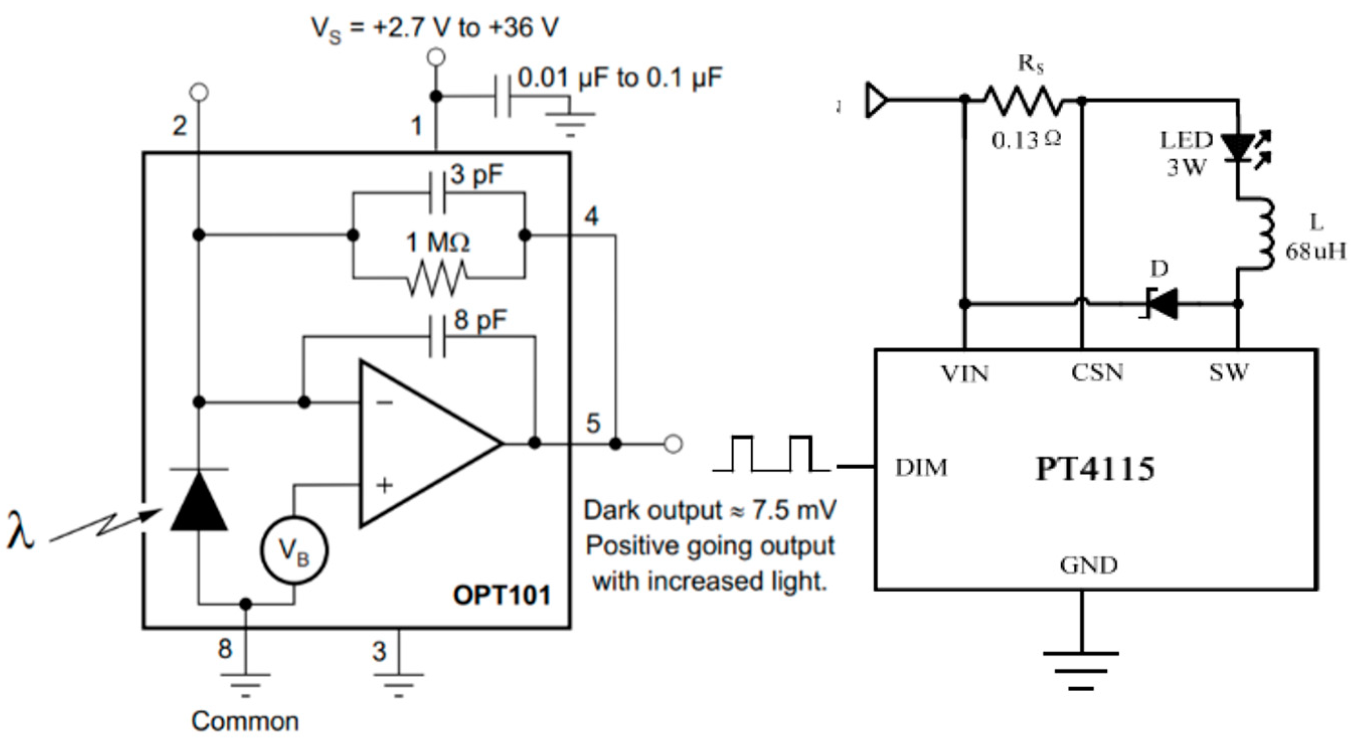
In terms of photosensitive devices, the accurate demodulation of high frequency poses a significant challenge for this project. Therefore, a photosensitive device with a high sensitivity requirement is needed. For this purpose, the PIN-type photodiode (PD) OPT101 [24] is selected, as illustrated in Figure 6. The OPT101 offers a spectral range of 300 nm to 1000 nm. It exhibits wide linear output characteristics, making it highly suitable for detecting visible light emitted by LED lights. This detector module integrates a photodiode and a transconductance amplifier, providing a voltage signal as the final output. Hence, the conversion of this signal into usable data requires an analog-to-digital (AD) conversion module. The detector module demonstrates high responsivity and low dark current. By utilizing external resistors and capacitors, the responsivity and sampling bandwidth of the module can be adjusted accordingly.
The LED lamp driving modulation module is a crucial component of the transmitter module. In this paper’s experiment, PWM modulation is utilized for LED modulation. The LED driver module controls the current through the PWM wave transmitted by the ESP32, thereby adjusting the luminous frequency and power of the LED lamp. To achieve this, we employ the PT4115 as our current control chip.
The PT4115 [25] is a continuous-mode inductive buck converter designed for the efficient driving of single or multiple series LEDs when the supply voltage exceeds the output voltage. The IC operates with an input voltage ranging from 5 V to 24 V, and the output current can be externally adjusted, with a maximum output current of 0.7 A. As depicted in Figure 6, the PT4115 integrates power tubes and a high-end current detection circuit. The average output current can be set using an external resistor. Additionally, the output current can be reduced below the set value by applying a DC voltage or PWM signal to the DIM pin. The DIM pin supports both linear and PWM dimming. Applying a voltage of 0.2 V or less to the DIM pin turns off the output power tube, putting the IC into low-current standby mode.
The ESP32 has the capability to register devices in a cloud platform [26], allowing for remote control and data upload as long as an internet connection is available. Cloud platforms can be categorized into three levels: infrastructure as a service (IaaS) as the underlying infrastructure, platform as a service (PaaS) in the middle layer, and software and services (SaaS) in the upper layer. The IoT cloud platform we employ is based on PaaS and follows the cloud service deployment model, typically categorized into public and non-public clouds (e.g., private cloud, hybrid cloud). Given the anticipated high number of simultaneous online users in this project, Ali Cloud is selected as our target cloud platform.
On the transmitter side, only the frequency and duty cycle of the LED need to be controlled, while the receiver may require extensive data uploading. To set up the ESP32 programming environment in the Arduino software (version 2.0.2), relevant support libraries such as Crypto, pubsubclient-2.8, and Arduino Json need to be downloaded. ESP-IDF also provides routines that allow for experimentation on both platforms.
Finally, on the transmitter side, the device is created on the Ali cloud platform, and the host computer program is written. The host computer can change the frequency and duty cycle of the relevant ESP32 to generate PWM waves by accepting input instructions. As shown in Figure 7, a single ESP32 can drive up to 4 LEDs at different frequencies and duty cycles. The maximum number of devices that the host computer can control depends solely on the equipment limit of Ali Cloud.
At the receiving end, a host computer based on TCP is built, which can receive 12,000 values sampled by ESP32 per second and convert them into CSV files, as shown in Figure 7.
Different components are spliced by drawing PCB using Jialichuang EDA platform. The PCB diagram and the physical diagram of the transmitter and receiver are shown in Figure 8. Then, the LED controlled by the transmitter is placed horizontally on the bracket, and the receiver is placed on the car. At this point, the hardware construction of the experiment in this paper is completed, and the overall experimental scenario is shown in Figure 9.

4. Diffusion Model in Real Scenes

The primary objective of this chapter is to obtain the parameters in each formula for real-world scenarios, aiming to establish the diffuse reflection model and line-of-sight (LOS) model for practical environments. In Equation (5), we need to determine two parameters, a i and b i , while in Equation (7), we need to determine two other parameters, m i and K i . Where m i = b i M 2 , m i can be calculated from b i .
Therefore, our idea is to first obtain the parameters a i and b i through Equation (5), and then obtain the parameter K i through Equations (7) and (8). The entire process is illustrated in Figure 10 and is explained later in the paper.
First, we obtain the parameters a i and b i . According to Equation (5), we will fit the relationship between RSS value and distance, based on the positions of selected points and their corresponding R S S L O S i values, as well as the positions of the LED, in the absence of wall reflections. This process is illustrated in Figure 10. Then, we obtain the parameters a i and b i for each LED. The fitting curve shown in Figure 11 indicates a high accuracy, with fitting errors ranging from 1.92 to 4.39 cm.
Thus, we obtained three sets of relationships between R S S L O S i and distance, thereby obtaining the parameters shown in Table 1.
The b i value provides m i for the computation of Equation (7).
Then we obtain the parameters K i . In the practical scenario, for ease of testing, we selected one line parallel to the wall and another perpendicular to the wall for testing purposes.
We can then subtract the R S S L O S i obtained in the occluded wall case from the R S S i obtained in the exposed wall case as a real R S S W a l l i to obtain the R S S W a l l i for the real scene. By adjusting through a suitable range of values K i in Equation (7), when mean error between the R S S W a l l i calculated by the model and the real R S S W a l l i are least, they are matched. At this point, K i represents the LED’s luminous intensity and the wall’s diffuse reflection ratio, denoted as K i in the context of the study.
Subsequently, we can assess the correctness of the parameters by using points from another parallel line, as shown in Figure 12. The red line is the R S S W a l l i calculated by the model, and the blue line is the R S S W a l l i obtained from the real scene. The average error of our model can reach 0.74% in the x-direction and 1.66% in the y-direction. We believe that such errors are sufficient to prove the correctness of our model in the presence of sampling fluctuations. The same operation will be performed on the other two LEDs. The optimal K values matched by the three LEDs are listed in Table 1.
After determining the aforementioned parameters, we obtain the single-lamp–single-wall model, as shown in Figure 13a. The variation along the y-axis, i.e., the change in received light intensity as the PD moves along a line parallel to the wall surface, is shown in Figure 13b. The variation along the x-axis, i.e., the change in received light intensity as the PD moves along a line parallel to the wall surface, is shown in Figure 13c. Figure 13d shows the diffuse reflection intensity of the wall observed from a top-down perspective, and it can be seen that it is attenuated outwardly centered at a point.
After completing the above preparations, we will conduct formal experiments under the conditions of uncovering and obstructing the wall. We will collect trajectory data separately for the obstructed and exposed wall surfaces, and then use the model we established to correct the trajectory data for the exposed wall surface. We will compare the corrected trajectory data with the standard trajectory data for the three aforementioned trajectories.

5. Experiments

5.1. Experimental Settings

As shown in Figure 9, we arranged a 1 m × 1 m × 1 m field. In order to minimize the occlusion of light on the light frame and apply it to our model as much as possible, we arranged two LEDs near the two corners of the wall, and one LED at the far end of the middle, forming a trilateral positioning.
In terms of signal modulation, in order to avoid harmonic interference and frequency instability, we choose three frequencies with fewer common factors, which are 1300 Hz, 1800 Hz, and 2300 Hz, respectively. The duty cycle is chosen to be 50%.
Since the bandwidth of OPT101 is 14 kHz, we choose 12 kHz as the sampling frequency, and the actual measurement shows that the frequency characteristics of the signal are good at this sampling frequency, which is suitable for Fourier transform.
In terms of measurement method, we will use the established trajectory on graph paper as the real trajectory and measure the RSS values under the conditions of shading cloth occlusion and without shading cloth occlusion, respectively, compare the results of the trilateral positioning without wall reflection, with wall reflection, and with wall reflection but optimized by the model, and use the distance between them and the real trajectory as the evaluation index. A smaller distance indicates a more accurate localization result.

5.2. Evaluation

We tested a total of two trajectories, as shown in Figure 14, where the green line represents the preset standard trajectory, the blue line represents the results of our trilateral localization under the wall occlusion condition, the red line represents the results of our trilateral localization under the wall exposure condition, and the yellow line represents the positioning results obtained after being optimized by our model.
To comprehensively evaluate our optimization capability, we employ several performance metrics, namely the mean error (ME) and root mean square error (RMSE), as well as errors corresponding to probability thresholds of 50% and 90%. Through the utilization of probability cumulative distribution function (CDF) analysis, we have discerned that our model exhibits consistent capacity to optimize received signal strength (RSS) values across diverse distances.
As shown in Table 2, under the condition of wall occlusion, the mean positioning errors of the two trajectories are 3.04 cm and 3.70 cm, the RMSEs of the two trajectories are 3.04 cm and 3.70 cm, 50% of the positioning errors are, respectively, within 3.59 cm and 3.38 cm, and 90% of the positioning errors are, respectively, within 5.55 cm and 5.03 cm, which are high-precision. However, after adding the diffuse reflection of the wall, the mean positioning errors of the two trajectories decreased to 13.37 cm and 14.73 cm, the RMSEs of the two trajectories reduced to 14.18 cm and 15.25 cm, 50% of the positioning errors are, respectively, within 13.72 cm and 14.84 cm, and 90% of the positioning errors are, respectively, within 19.68 cm and 20.97 cm. Thus, the reflection of the wall seriously decreases the positioning precision.
After introducing the wall diffuse reflection model, our positioning results achieve impressive enhancement in accuracy ranging from 36.7% to 61.3% when confronted with the presence of diffuse reflection occurring on the wall. Specifically, the mean positioning errors of the two trajectories decreases to 6.20 cm and 6.19 cm, the RMSE of the two trajectories decreases to 6.98 cm and 6.88 cm, 50% of the positioning errors are, respectively, within 5.45 cm and 5.74 cm, and 90% of the positioning errors are, respectively, within 12.46 cm and 8.64 cm. Thus, our method has brought the positioning precision back to a relatively precise state when faced with the reflection of the wall. The detail can also be found in the CDF figures, as shown in Figure 15. Our method (blue line) achieves a better performance than the method without consideration of the diffuse reflection (red line).
We believe that the positioning results of this system can achieve such accuracy, first of all, thanks to the miniaturization, simplification, high stability, and good anti-sidelobe effect of the system, which makes its positioning effect ideal in the state of low interference. The second reason is that the scene we built is relatively small and ideal, and we can accurately obtain the values of each parameter, which is difficult to do in actual scenes. Expanding the model in complex scenarios is one of the next steps in our research agenda.

6. Discussion

In attempting to address this issue, during our preliminary research, we found that, although there are numerous articles studying visible light localization with wall diffuse reflection, most of them conducted only simulations and had limited validation in real-world scenarios. This makes it challenging for us to make direct comparisons. In Table 3, we provide a representative summary of other studies’ results. It is essential to note that the settings and objectives of these works are not entirely identical. We present them here merely to provide a rough comparation.
For instance, in Study 1 [16], the scene size was 4 m × 4 m × 3 m, with 80% of positioning errors being smaller than 7.88 cm and 95% of positioning errors being smaller than 9.87 cm. Since they did not present improvements brought about by their model, we can use only positioning errors as the basis for our evaluation. However, they evaluate their model only in simulated scenes, and there remains a significant gap between real-world validation and simulations. From the distribution of our cumulative distribution function (CDF), it can be observed that there is a certain gap between the performance of sensors at some distant points and those at close range. In reality, factors such as wall uniformity, unexpected obstructions, communication stability, and the quality of chip oscillators can significantly influence the positioning results. Under the influence of these various factors, we achieved positioning accuracy similar to simulations and even outperformed some larger scenes by an order of magnitude. We believe this is sufficient to demonstrate the model’s usability in real-world scenarios and can provide a reference for future experiments with other models in practical environments. Moreover, other methods in Table 3 were verified only in simulated scenes; consequently, they have similar characteristics and results.

7. Conclusions

We have developed a visible light positioning system based on the ESP32 microcontroller, an Internet of Things (IoT) platform, and the received signal strength (RSS) technique. This system exhibits notable advantages in terms of compactness, affordability, stability, and resistance to sidelobe interference, thus presenting a promising avenue for the future commercialization of visible light positioning. In order to address the significant concern of wall reflections in indoor visible light positioning, we have formulated and simulated a model, verifying its feasibility through practical implementation.
Nevertheless, it is important to note that the constructed scene in our study is a simplified environment, only with 1 × 1 × 1 m3 size, whereas our modeling work will encounter more complex wall geometry features and higher environmental noise in larger scenarios. The current research work lacks comprehensive reflection modeling in large-scale complex scenes. Hence, future endeavors will involve the utilization of more robust methodologies to tackle the issue of wall reflections in larger and more intricate settings. Here, we present two suggestions:
  • For the challenging task of modeling geometric features on large-scale wall surfaces, we recommend utilizing Lidar technology to measure planar scenes. This approach will enable stable and efficient modeling for various scenarios;
  • Existing physics-based models cannot meet our real-time computational speed requirements. Therefore, we recommend the development of more efficient methods for fitting existing physics equations.
Expanding this model is also one of our further objectives.

Author Contributions

Conceptualization, X.Y., X.S. and Y.Z. (Yuan Zhuang); Methodology, Y.Z. (Yuanpeng Zhang) and X.Y.; Software, Y.Z. (Yuanpeng Zhang); Validation, Y.Z. (Yuanpeng Zhang); Formal analysis, Y.Z. (Yuanpeng Zhang) and Y.W.; Investigation, X.S.; Data curation, Y.W.; Writing—original draft, Y.Z. (Yuanpeng Zhang); Writing—review & editing, X.Y.; Project administration, T.M. and Y.Z. (Yuan Zhuang); Funding acquisition, T.M. All authors have read and agreed to the published version of the manuscript.

Funding

This work is supported by the Special Fund of Anhui University of Science and Technology (SKLMRDPC21KF20), the Excellent Youth Foundation of Hubei Scientific Committee (2021CFA040), and the Knowledge Innovation Program of Wuhan-Shuguang Project under Grant (2022020801020128).

Data Availability Statement

Not applicable.

Conflicts of Interest

The authors declare no conflict of interest.

References

  1. Li, Q.; Yao, W.; Tu, R.; Du, Y.; Liu, M. Performance Assessment of Multi-GNSS PPP Ambiguity Resolution with LEO-Augmentation. Remote Sens. 2023, 15, 2958. [Google Scholar] [CrossRef]
  2. Özsoy, K.; Bozkurt, A.; Tekin, I. 2D Indoor positioning system using GPS signals. In Proceedings of the 2010 International Conference on Indoor Positioning and Indoor Navigation, Zurich, Switzerland, 15–17 September 2010; pp. 1–6. [Google Scholar]
  3. Xu, Q.; Gao, Z.; Yang, C.; Lv, J. High-Accuracy Positioning in GNSS-Blocked Areas by Using the MSCKF-Based SF-RTK/IMU/Camera Tight Integration. Remote Sens. 2023, 15, 3005. [Google Scholar] [CrossRef]
  4. Yang, X.; Zhuang, Y.; Gu, F.; Shi, M.; Cao, X.; Li, Y.; Zhou, B.; Chen, L. DeepWiPos: A Deep Learning-Based Wireless Positioning Framework to Address Fingerprint Instability. IEEE Trans. Veh. Technol. 2023, 72, 8018–8034. [Google Scholar] [CrossRef]
  5. Zhuang, Y.; Yang, J.; Li, Y.; Qi, L.; El-Sheimy, N. Smartphone-Based Indoor Localization with Bluetooth Low Energy Beacons. Sensors 2016, 16, 596–615. [Google Scholar] [CrossRef] [PubMed]
  6. Fang, S.H.; Wang, C.H.; Huang, T.Y.; Yang, C.H.; Chen, Y.S. An Enhanced ZigBee Indoor Positioning System with an Ensemble Approach. IEEE Commun. Lett. 2012, 16, 564–567. [Google Scholar] [CrossRef]
  7. Gu, W.; Zhang, W.; Kavehrad, M.; Feng, L. Three-dimensional light positioning algorithm with filtering techniques for indoor environments. Opt. Eng. 2014, 53, 107107. [Google Scholar] [CrossRef]
  8. Singh, P.; Jeon, H.; Yun, S.; Kim, B.W.; Jung, S.Y. Vehicle Positioning Based on Optical Camera Communication in V2I Environments. CMC-Comput. Mater. Contin. 2022, 72, 2927–2945. [Google Scholar] [CrossRef]
  9. Li, N.; Liu, C.; Pfeifer, N. Improving LiDAR classification accuracy by contextual label smoothing in post-processing. ISPRS J. Photogramm. Remote Sens. 2019, 148, 13–31. [Google Scholar] [CrossRef]
  10. Müller, P.; Wymeersch, H.; Piché, R. UWB Positioning with Generalized Gaussian Mixture Filters. IEEE Trans. Mob. Comput. 2014, 13, 2406–2414. [Google Scholar] [CrossRef]
  11. Zhuang, Y.; Hua, L.; Qi, L.; Yang, J.; Cao, P.; Cao, Y.; Wu, Y.; Thompson, J.; Haas, H. A Survey of Positioning Systems Using Visible LED Lights. IEEE Commun. Surv. Tutor. 2018, 20, 1963–1988. [Google Scholar] [CrossRef]
  12. Sun, X.; Zhuang, Y.; Huai, J.; Hua, L.; Chen, D.; Li, Y.; Cao, Y.; Chen, R. RSS-Based Visible Light Positioning Using Nonlinear Optimization. IEEE Internet Things J. 2022, 9, 14137–14150. [Google Scholar] [CrossRef]
  13. Chan, H.M.; Chow, C.-W.; Hsu, L.-S.; Liu, Y.; Peng, C.-W.; Jian, Y.-H.; Yeh, C.-H. Utilizing Lighting Design Software for Simulation and Planning of Machine Learning Based Angle-of-Arrival (AOA) Visible Light Positioning (VLP) Systems. IEEE Photonics J. 2022, 14, 1–7. [Google Scholar] [CrossRef]
  14. Jung, S.Y.; Hann, S.; Park, C.S. TDOA-based optical wireless indoor localization using LED ceiling lamps. IEEE Trans. Consum. Electron. 2011, 57, 1592–1597. [Google Scholar] [CrossRef]
  15. Mohammed, N.A.; Elkarim, M.A. Exploring the effect of diffuse reflection on indoor localization systems based on RSSI-VLC. Opt. Express 2015, 23, 20297–20312. [Google Scholar] [CrossRef]
  16. Yang, W.J.; Qin, L.; Hu, X.L.; Zhao, D.S. Indoor Visible-Light 3D Positioning System Based on GRU Neural Network. Photonics 2023, 10, 633. [Google Scholar] [CrossRef]
  17. Gu, W.J.; Aminikashani, M.; Deng, P.; Kavehrad, M. Impact of Multipath Reflections on the Performance of Indoor Visible Light Positioning Systems. J. Light. Technol. 2016, 34, 2578–2587. [Google Scholar] [CrossRef]
  18. Hosseinianfar, H.; Noshad, M.; Brandt-Pearce, M. Positioning for Visible Light Communication System Exploiting Multipath Reflections. In Proceedings of the 2017 IEEE International Conference on Communications (ICC), Paris, France, 21–25 May 2017. [Google Scholar]
  19. Komine, T.; Nakagawa, M. Fundamental analysis for visible-light communication system using LED lights. IEEE Trans. Consum. Electron. 2004, 50, 100–107. [Google Scholar] [CrossRef]
  20. Huang, H.; Feng, L.; Guo, P.; Yang, A.; Ni, G. Iterative positioning algorithm to reduce the impact of diffuse reflection on an indoor visible light positioning system. Opt. Eng. 2016, 55, 066117. [Google Scholar] [CrossRef]
  21. Yu, M.; Chai, S. Iteration-dependent High-order Internal Model based Iterative Learning Control for Continuous-time Nonlinear Systems. In Proceedings of the 2020 IEEE 9th Data Driven Control and Learning Systems Conference (DDCLS), Liuzhou, China, 20–22 November 2020; pp. 1021–1025. [Google Scholar]
  22. Babiuch, M.; Foltýnek, P.; Smutný, P. Using the ESP32 Microcontroller for Data Processing. In Proceedings of the 2019 20th International Carpathian Control Conference (ICCC), Kraków-Wieliczka, Poland, 26–29 May 2019; pp. 1–6. [Google Scholar]
  23. Dian, F.J.; Yousefi, A.; Lim, S. A practical study on Bluetooth Low Energy (BLE) throughput. In Proceedings of the 2018 IEEE 9th Annual Information Technology, Electronics and Mobile Communication Conference (IEMCON), Vancouver, BC, Canada, 1–3 November 2018; pp. 768–771. [Google Scholar]
  24. Vidya, M.J.; Padmaja, K.V.; Chaithra, G. An indigenous PPG acquisition system using monolithic photo-detector OPT101. In Proceedings of the 2016 International Conference on Signal Processing, Communication, Power and Embedded System (SCOPES), Paralakhemundi, India, 3–5 October 2016; pp. 1457–1460. [Google Scholar]
  25. He, X.; Wang, H.; Cao, J.; Lei, D. Design of High-power LED Automatic Dimming System for Light Source of On-line Detection System. In Proceedings of the 2020 IEEE 5th Information Technology and Mechatronics Engineering Conference (ITOEC), Chongqing, China, 12–14 June 2020; pp. 1487–1491. [Google Scholar]
  26. Saraswat, M.; Tripathi, R.C. Cloud Computing: Analysis of Top 5 CSPs in SaaS, PaaS and IaaS Platforms. In Proceedings of the 2020 9th International Conference System Modeling and Advancement in Research Trends (SMART), Moradabad, India, 4–5 December 2020; pp. 300–305. [Google Scholar]
Figure 1. The overall system diagram.
Electronics 12 03646 g001
Figure 2. A schematic diagram of the line-of-sight (LOS) and wall diffuse reflection.
Electronics 12 03646 g002
Figure 3. The principle of RSS trilateral positioning.
Electronics 12 03646 g003
Figure 4. Positioning process.
Electronics 12 03646 g004
Figure 5. Main control chip (ESP32) example.
Electronics 12 03646 g005
Figure 6. OPT101 example & PT4115 example.
Electronics 12 03646 g006
Figure 7. Transmitter control interface and receiver data format.
Electronics 12 03646 g007
Figure 8. PCB diagram and physical diagram.
Electronics 12 03646 g008
Figure 9. Overall experimental scenario.
Electronics 12 03646 g009
Figure 10. The process for parameter determination.
Electronics 12 03646 g010
Figure 11. Fitted curve.
Electronics 12 03646 g011
Figure 12. Comparison of model calculations and actual values.
Electronics 12 03646 g012
Figure 13. Wall diffuse reflection model.
Electronics 12 03646 g013
Figure 14. The three positioning results are compared with the standard trajectory.
Electronics 12 03646 g014
Figure 15. CDF positioning error.
Electronics 12 03646 g015
Table 1. Coefficient obtained by fitting.
LED Parameters   Obtained   by   Fitting   ( R S S L O S = a · d b )
abK
LED18.1939−0.3047799.1
LED28.5522−0.3134798.5
LED39.3178−0.3264785.3
Table 2. Positioning errors.
Error
Trajectory Type of Error No Diffusion
(cm)
Diffusion Existed
(cm)
Our Results
(cm)
Improvement
(%)
Trajectory1ME3.7013.376.2053.63
RMSE4.0414.186.9850.78
50%3.5913.725.4560.28
90%5.5519.6812.4636.69
Trajectory2ME3.0414.736.1957.98
RMSE3.4015.256.8854.89
50%3.3814.845.7461.32
90%5.0320.978.6458.80
Table 3. Comparison with other studies’ results.
ThesisMethods and ApproachesSceneEvaluation MetricsNumerical Value (Unit)Simulation or
Real-World
Experiment
Study 1 [16]Visible light positioning (VLP);
line-of-sight (LOS) and non-line-
of-sight (NLOS) links;
gated recurrent units (GRU) neural networks
80% of the positioning errors7.88 (cm)Simulation
2 LEDs
4 m × 4 m × 3 m
95% of the positioning
errors
9.87 (cm)
Study 2 [17]Visible light positioning (VLP);
multipath reflections;
received signal strength (RSS);
16 LEDs
8 m × 8 m × 2.3 m
Root Mean
Square Error (RMSE) (the best of all conditions)
31.69 (cm)Simulation
Study 3 [18]Visible light indoor positioning; multipath reflections; maximum likelihood estimation4 PDs
5 m × 5 m × 3 m
Root Mean
Square Error (RMSE)
5 (cm)Simulation
Study 4 [15]Received signal strength indication (RSSI); visible
light communication (VLC)
4 LEDs
5 m × 5 m × 3 m
Root Mean
Square Error (RMSE)
68 (cm)Simulation
Our StudyVisible light positioning (VLP);
line-of-sight (LOS) and non-line-
of-sight (NLOS) links;
iteration
3 LEDs
1 m × 1 m × 1 m
80% of the positioning errors7.81 (cm)Real-world
Experiment
95% of the positioning
errors
13.46 (cm)
Root Mean
Square Error (RMSE)
6.88 (cm)
Disclaimer/Publisher’s Note: The statements, opinions and data contained in all publications are solely those of the individual author(s) and contributor(s) and not of MDPI and/or the editor(s). MDPI and/or the editor(s) disclaim responsibility for any injury to people or property resulting from any ideas, methods, instructions or products referred to in the content.

