Neural Network Approach Super-Twisting Sliding Mode Control for Path-Tracking of Autonomous Vehicles

Abstract

This paper proposes a neural network approach adaptive super-twisting sliding mode control algorithm for autonomous vehicles. An adaptive and robust control algorithm in autonomous vehicles is needed to compensate for disturbance and parametric uncertainty from the variable environment and vehicle conditions. The sliding mode control (SMC) is a robust controller that compensates for robust and reasonable control performance against disturbance and parametric uncertainty. However, the inherent limitation of the sliding mode control, namely the chattering phenomenon, has a negative effect on the system. Additionally, when the disturbance exceeds the defined boundaries, the control stability is compromised. To overcome these limitations, this study incorporates the radial basis function neural network (RBFNN) and Lyapunov function to estimate disturbance and parametric uncertainty. The estimated disturbance is reflected in the super-twisting sliding mode control (STSMC) to reduce the chattering phenomenon and achieve enhanced robust performance. The performance evaluation of the proposed neural network approach control algorithm is conducted using the double lane change (DLC) scenario and rapid path-tracking (RPT) scenario, implemented in the CarMaker and Matlab/Simulink environments, respectively.

1. Introduction

In recent years, automated and intelligent systems have been developed and implemented across various industries to enhance user convenience and safety. This trend has also influenced the automotive industry, where extensive research on various autonomous driving technologies is being conducted worldwide to achieve high efficiency and performance. Autonomous driving control techniques can be divided into longitudinal and lateral controls, with implications for driving stability and driving comfort. The lateral control is closely related to path-tracking problems and uses independent driving and steering systems, with steer-by-wire (SBW) and drive-by-wire (DBW) systems. Various control theories are being developed and applied for the chassis control of autonomous vehicles, with classic control, modern control, and learning-based control algorithms being actively researched in universities and research institutions.

Saruchi et al. (2020) proposed a fuzzy proportional–integral–derivative (PID) control for motion sickness (MS) minimization control structure that adopted the interaction of lateral acceleration and the head tilt concept to minimize MS [1]. Kebbati et al. (2021) implemented an adaptive PID control using a genetic algorithm and neural network approaches for longitudinal control in autonomous vehicles [2]. Azar et al. (2019) applied a PID control for automated parking and utilized the particle-swarm optimization (PSO) method for tuning the appropriate gain values [3]. Max et al. (2018) considered uncertainties in autonomous vehicles using the SBW system and evaluated the performance using the robust H-infinity control through hardware-in-the-loop-simulation (HILS) [4]. Guo et al. (2020) proposed a robust H-infinity fault-tolerant state feedback lateral control algorithm to compensate for the steering-wheel failure of an autonomous vehicle with a four-wheel independent steering system and to secure path-tracking performance [5]. Li et al. (2017) presented a distributed H-infinity control for platooning in autonomous vehicles, ensuring robust stability, tracking performance, and heterogeneous string stability [6]. Park et al. (2021) proposed a control method for self-driving cars that enables drift maneuvers for fast cornering. Park’s proposed feedback control algorithm was designed using a linear quadratic regulator (LQR) to track a circular trajectory and maintain the drift equilibrium state [7]. Guo et al. (2021) applied extended state observer (ESO)-based LQR for the path following an autonomous bus. The ESO was utilized to estimate the dynamics and model uncertainties of the bus in real time, with the estimated disturbance being incorporated into the LQR for path tracking [8]. Gonschorek et al. (2022) proposed modeling, control synthesis, control loop analysis, and vehicle performance evaluation for position control of the front-axle actuator of the SBW system. To control of the SBW system, a linear quadratic Gaussian control was designed using a linearized model of the SBW system [9]. Lee et al. (2019) introduced an adaptive q-matrix-based linear quadratic Gaussian (LQG) control algorithm for path tracking in autonomous vehicles, aiming to minimize errors and noise in localization and path planning. To confirm the performance of Lee’s proposed control algorithm, it was compared with pure pursuit and the Stanley method [10]. Peng et al. (2020) proposed a model predictive control (MPC) with a finite time horizon for path tracking and direct yaw moment control (DYC) implementation in four-wheeled autonomous driving vehicles [11]. Wang et al. (2021) utilized recursive least squares (RLS) to estimate cornering stiffness, which incorporates time-varying uncertainties, in real time for path tracking in autonomous vehicles equipped with a four-wheel independent driving system. The estimated parameters were then used to design an adaptive model predictive control (AMPC) [12]. Chen et al. (2020) designed an MPC to ensure autonomous vehicle path-tracking performance and handling stability in extreme conditions by considering multiple constraint conditions [13]. Pang et al. (2022) presented a linear time-varying model predictive control (LTV-MPC) approach based on a vehicle kinematic model for autonomous path tracking [14]. Cheng et al. (2020) proposed a linear matrix inequality model predictive control (LMI-MPC) to compensate for the performance degradation caused by parametric uncertainty and time-varying factors [15]. To ensure path-tracking performance, various control algorithms, such as classical control, robust control, optimal control, and predictive control, have been applied [1,2,3,4,5,6,7,8,9,10,11,12,13,14,15]. The disturbances and uncertainties that can affect autonomous vehicles, such as tire nonlinearity, vehicle parameters, and sensor noise, lead to performance degradation. Therefore, various adaptive algorithms based on learning and estimation techniques have been proposed to compensate for the control performance of autonomous vehicles. These adaptive algorithms involve the real-time tuning of control gains or the estimation of parameters that incorporate disturbance and parametric uncertainty in the system [2,3,7,10,12].

Liang et al. (2020) proposed a variable-speed method based on sliding mode and a second-order quasi-continuous (QC) method based on the path-tracking algorithm considering the friction limit of the road surface, for clothoid-based path-tracking [16]. Tagne et al. (2013) proposed a high-order sliding mode control (HOSMC) for the lateral control of autonomous vehicles. HOSMC was proposed to reduce the chattering phenomenon, a limitation of SMC, while utilizing the robustness of SMC against model nonlinearity and parametric uncertainty [17]. Wang et al. (2016) proposed an adaptive sliding mode control (ASMC) with a Takagi–Sugeno (T–S) fuzzy model to account for the changing cornering stiffness in extreme handling situations and to represent the tire nonlinearity and the nonlinearity of the control input [18]. Ferrara et al. (2019) presented an adaptive optimization-based second-order sliding mode control (SOSMC) to ensure finite time convergence and robust control in uncertain nonlinearities in autonomous vehicles while minimizing control effort [19]. Hu et al. (2016) proposed a super-twisting algorithm (STA)-based integral sliding mode control (ISMC) for the path-following control of a four-wheel independent-driving autonomous vehicle through active front steering (AFS) and DYC [20]. Xu et al. (2017) proposed a model-free adaptive sliding mode control (MF-ASMC) for the parking systems of autonomous vehicles, incorporating the online identification of the object model and constraints on control inputs based on data-driven techniques [21]. Bei et al. (2022) presented an integrated adaptive preview control with SOSMC for path-tracking autonomous vehicles, comparing its performance with MPC [22]. Rivera et al. (2011) described the application of the STA in motion-control systems to compensate for performance degradation caused by the chattering phenomenon, a limitation of SMC [23]. Kang et al. (2017) proposed a lateral control algorithm for the lanekeeping of autonomous vehicles by estimating lateral velocity based on a second-order linear dynamic model and utilizing backstepping [24]. Ao et al. (2021) developed a super-twisting sliding mode control (STSMC) based on Lyapunov theory to achieve robust path tracking and reduce the chattering phenomenon in autonomous vehicles, demonstrating the stability of the control system through the application of backstepping [25]. Norouzi et al. (2019) designed the backstepping-based SMC, defined the Lyapunov function, and proved its stability. Norouzi’s proposed control algorithm confirmed reasonable performance compared with the backstepping control at low road friction [26]. Wang et al. (2019) proposed a vehicle–road system model and designed a backstepping-based SMC, robust to disturbance and time-varying factors, for autonomous vehicles [27]. SMC is a robust control against disturbance and parametric uncertainty. However, it can cause system overload and failure due to the chattering phenomenon [17,23,25]. In addition, it has a limitation that control stability is lost due to excessive nonlinearity in the system [16,17,18]. To overcome these limitations, various control methods have been proposed, such as SMC, SOSMC, and HOSMC with backstepping [16,17,18,19,20,21,22,23,24,25,26,27].

Wang et al. (2019) proposed SMC based on RBFNN to reduce the speed tracking error and chattering phenomenon in the longitudinal control of autonomous vehicles [28]. Sun et al. (2020) presented an integrated terminal sliding mode control (ITSMC) based on neural networks for collision avoidance steering control in autonomous vehicles. RBFNN was utilized to approximate the upper bound of system uncertainties online without requiring prior knowledge, thereby achieving robust control performance [29]. In another work by Sun et al. (2022) the authors proposed a dual-hidden-layer output feedback neural network for the fast nonsingular terminal sliding mode control (FNTSMC) The proposed control algorithm for autonomous lateral control utilized a neural network model to estimate parametric uncertainties and achieved robust control performance [30]. Swain et al. (2021) addressed the chattering phenomenon in SMC and reduced the impact of external disturbance by using RBFNN to estimate the equivalent control input, along with proposing a high-order sliding mode-based switching control algorithm [31]. Ji et al. (2018) proposed a robust lateral control algorithm and a neural network approximator to maintain yaw stability in autonomous vehicles, considering the tire’s nonlinearity and external disturbance under various driving conditions [32]. Negash et al. (2022) proposed platoon control using an adaptive radial basis function neural network (ARBFNN)-based SMC to track the course and optimal speed of an autonomous vehicle [33]. Chen et al. (2021) constructed a vehicle control architecture for autonomous lateral control by combining deep reinforcement learning (DRL) with proximal policy optimization (PPO) and pure pursuit [34]. Zhang et al. (2018) proposed a double Q-learning-based reinforcement learning approach for longitudinal speed control in vehicles using naturalistic driving data, demonstrating reasonable control performance compared to a deep Q-learning algorithm [35]. Ma et al. (2018) enhanced and improved the existing game theory framework by adding noncompetitive incentives to dynamically adjust the disturbance magnitude and evaluated the efficiency and safety tradeoff for autonomous driving [36]. Kwon et al. (2022) proposed a lateral control methodology for autonomous vehicles that utilizes behavior cloning through an end-to-end learning system, making use of the driver data. Their proposed control algorithm was evaluated through various simulator environments [37]. Chai et al. (2022) proposed a real-time trajectory planning and tracking framework for autonomous vehicles. To approximate the optimal parking trajectory, motion planning was performed using a deep neural network (DNN) using a recurrent neural network (RNN) structure [38]. Tang et al. (2022) proposed a weight adaptation model predictive control system using a particle-swarm optimization back-propagation (PSO-BP) neural network to follow the path of an autonomous vehicle at various vehicle speeds and curvatures [39]. Huang et al. (2023) proposed a differentiable integrated prediction and planning framework that utilizes neural networks to predict the future state of nearby traffic participants, safe trajectories, and path planning for autonomous vehicles [40]. Wang et al. (2022) collected data by establishing a driving environment with an autonomous vehicle and a human driver for the car-following behavior of autonomous vehicles and performed velocity control using a soft actor-critic (SAC) algorithm [41]. Zhang et al. (2022) proposed a receding horizon reinforcement learning approach for the kino-dynamic motion planning (RHRL-KDP) of autonomous vehicles in the presence of inaccurate dynamics information and moving obstacles [42]. Xiao et al. (2023) applied the deep Koopman operator for the nonlinear dynamic modeling of an autonomous vehicle and designed a linear model predictive control based on the resulting model to perform longitudinal and lateral control [43]. Shi et al. (2022) propose a deep reinforcement learning (DRL)-based distributed longitudinal control strategy for connected and automated vehicles under communication failure to stabilize traffic oscillations [44]. Geng et al. proposed a neural network predictive control algorithm based on a back-propagation neural network using PSO with fitness-allocating inertia weights and examined the autonomous driving path-following problem in high-speed turning conditions [45]. Various research studies have been conducted on learning-based control algorithms, including artificial neural networks (ANN), RNN, DNN, and DRL. In addition, various studies, including path planning and end-to-end neural networks, have been conducted [38,40,42]. As can be seen in this control approach, it was confirmed that the predetermination of the parameters constituting the neural network was important, as was the identification of the appropriate training dataset for neural network learning [25,26,27,28,29,30,31,32,33,34,35,37,39,41,43,44,45]. RBFNN has been proposed in various methodologies to compensate for system disturbance and parametric uncertainty, as well as to address the chattering phenomenon in sliding mode controllers [28,29,30,31,32,33].

The definition of a mathematical model representing the physical characteristics of the system is crucial for achieving reasonable control performance with sliding mode controllers. However, there is a limitation when applying an unreasonable mathematical model along with the previously mentioned chattering phenomenon and excessive disturbances, which can lead to the loss of control stability. To overcome these limitations, methodologies have been proposed that combine fuzzy logic and ANN to estimate disturbances in control systems and enhance control performance. Among these, RBFNN stands out for its simplicity and ease of design [46]. 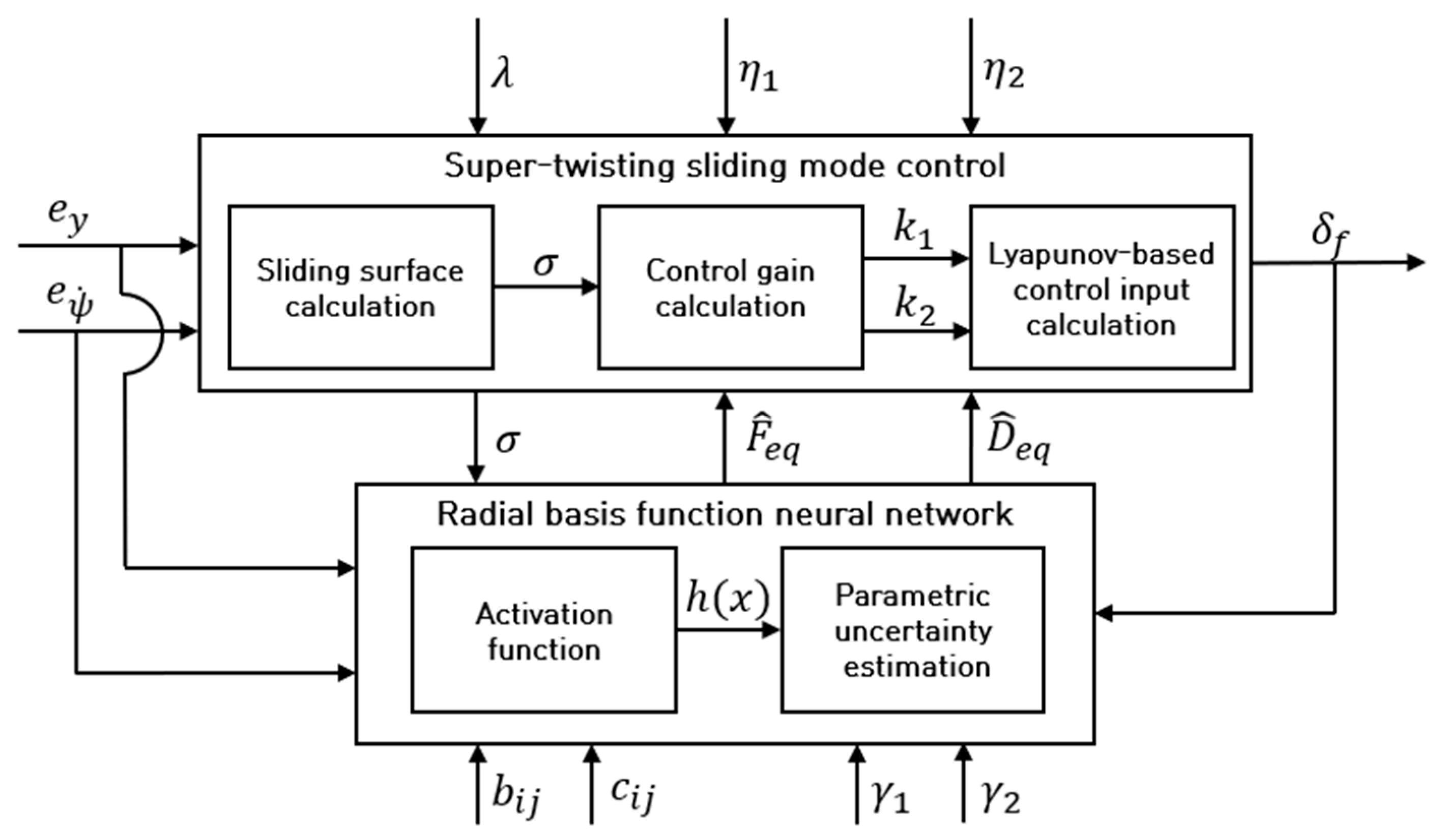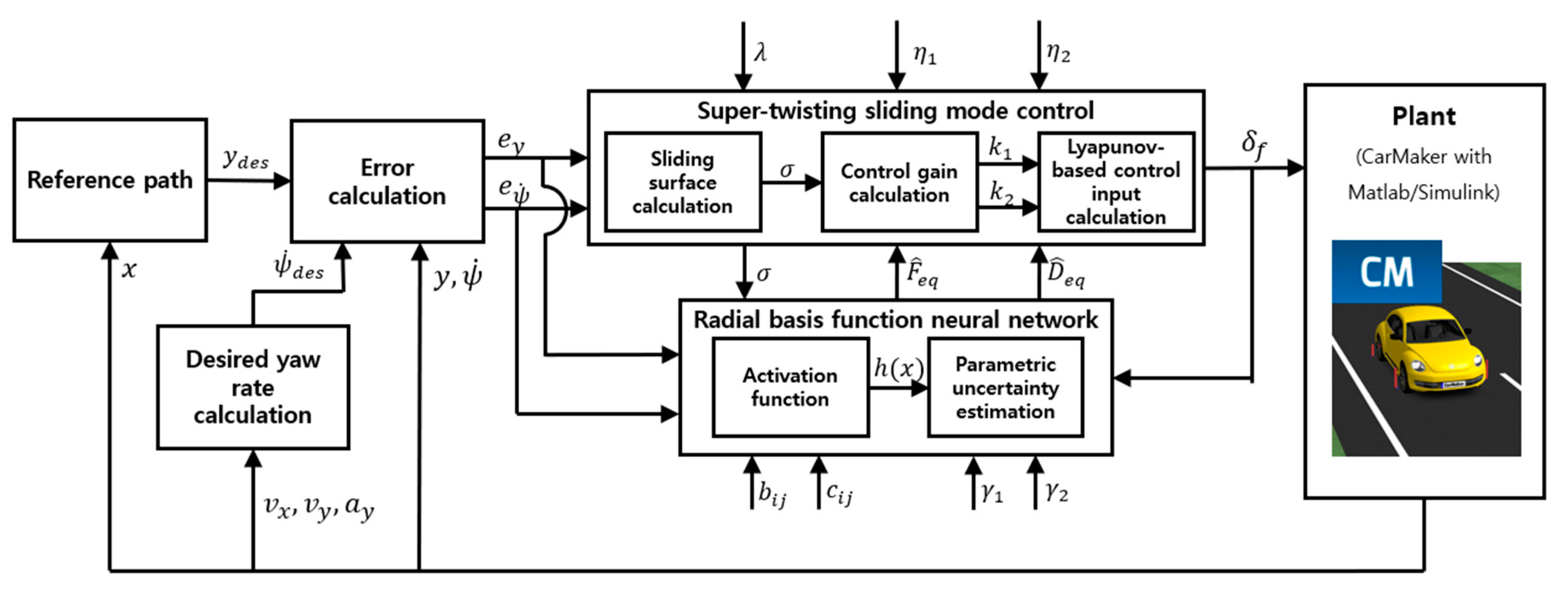STSMC has been developed to enhance the robustness of sliding mode controllers and reduce the chattering phenomenon [24,25]. For achieving reasonable and safe autonomous driving, defining the mathematical model of the system, and determining appropriate control gain values are essential. In this study, to approach the path-tracking method in autonomous vehicles with more robustness and adaptation, a learning-based robust control algorithm was proposed. This control algorithm contains the STSMC, which offers higher robustness and reduces chattering attenuation compared to SMC, with the RBFNN for estimating parametric uncertainty and disturbances. The contributions of the proposed research are outlined below:

• The STSMC is proposed for the robust path-tracking of autonomous vehicles. This controller is utilized to reduce chattering and improve driving stability. The stability proof of the proposed controller is proven using the Lyapunov method, and conditions for the control gain values are derived.
• RBFNN is designed to estimate parametric uncertainties and disturbances in autonomous vehicles. By using the Lyapunov method, the RBFNN is combined with the STSMC, ensuring parameter estimation and stability proof.
• By using estimated parameters, including parametric uncertainties and disturbances, the steering control input is adaptively adjusted in real time with the control gain. This adaptive rule ensures effective responses to variations in system dynamics and uncertainties.

2. Neural Network Approach Super-Twisting Sliding Mode Control

Figure 1 presents the overall block diagram of the proposed neural network approach super-twisting sliding mode control (NN-STSMC) for the autonomous driving path tracking in this study. To design the proposed control algorithm, a sliding surface is constructed based on the lateral error and the yaw-rate error, derived from the vehicle dynamic model. The control input is determined by utilizing the robust term and the steering-wheel input on the sliding surface, satisfying the Lyapunov negative definite condition. To account for disturbance and uncertainty in vehicle conditions, the parameters are estimated in real time using the RBFNN and the Lyapunov function. The estimated parameters are then reflected in the control gains and control input terms to ensure the Lyapunov stability conditions. In the following section, the derivation process of the vehicle’s lateral error dynamics model is described.

2.1. Vehicle Lateral Error Dynamics Model

This section explains a description of the derivation of the lateral error dynamic model. Figure 2 presents the vehicle’s lateral motion using a linear 2-DOF vehicle-dynamics model. The lateral and yaw dynamics models based on Newton’s second law can be designed as Equations (1) and (2), respectively. In Equation (1), $\ddot{y}$ represents the acceleration in the y-axis direction, while $v_x\dot{\psi }$ represents the centripetal acceleration.

$$m\left(\ddot{y}+v_x\dot{\psi }\right)=F_{yf}+F_{yr}$$

(1)

$$I_z\ddot{\psi }=l_f{F}_{yf}-l_r{F}_{yr}$$

(2)

where $y$, $v_x$, and $\psi$ represent the lateral position, longitudinal velocity, and yaw angle, respectively. The parameters $m$, $I_z$, $l_f$, and $l_r$ denote the vehicle’s mass, yaw inertia, and distances from the vehicle’s center of mass to the front and rear axes, respectively. $F_{yf}$ and $F_{yr}$ correspond to front-wheel lateral tire force and rear-wheel lateral tire force, respectively. The expressions for $F_{yf}$ and $F_{yr}$ in Equations (1) and (2) involve the front and rear cornering stiffness coefficients $C{}_f$ and $C{}_r$, the wheel slip angles ${\alpha }_f$ and ${\alpha }_r$, and the wheel steering angle ${\delta }_f$.

$$F_{yf}=C_f{\alpha }_f=C{}_f\left({\delta }_f-\frac{v_y+l_f\dot{\mathsf{\psi }}}{v_x}\right)$$

(3)

$$F_{yr}=C_r{\alpha }_r=C{}_r\left(-\frac{v_y-l_r\dot{\psi }}{v_x}\right)$$

(4)

The desired yaw rate, ${\dot{\psi }}_{des}$, can be formulated using the longitudinal velocity $v_x$ and the turning radius. The turning radius, $R$, is the reciprocal of the curvature, $\kappa$, of the driving path and can be expressed in terms of lateral velocity and lateral acceleration.

$${\dot{\psi }}_{des}=v_x\kappa$$

(5)

$$\kappa =\frac{1}{R}=\frac{\ddot{ y}}{\sqrt[3]{{(1+\dot{y})}^2}}$$

(6)

The derivatives of the lateral error, ${\dot{e}}_y$, and the yaw-rate error, ${\dot{e}}_{\psi }$, can be defined through Equations (7) and (8), respectively. By using Equations (1)–(4), (7), and (8), the lateral error dynamics model can be derived as Equation (9) and the yaw-rate error dynamics model can be derived through Equation (10).

$${\dot{e}}_y=\dot{y}+v_x(\psi -{\psi }_{des})$$

(7)

$${\dot{e}}_{\psi }=\dot{\psi }-{\dot{\psi }}_{des}$$

(8)

$${\ddot{e}}_y=-\frac{2C_f+2C_r}{m{v}_x}{\dot{e}}_y+\frac{2C_f+2C_r}{m}{e}_{\psi }+\frac{-2C_f{l}_f+2C_r{l}_r}{m{v}_x}{\dot{e}}_{\psi }+\left(-\frac{2C_f{l}_f-2C_r{l}_r}{m{v}_x}-v_x\right){\dot{\psi }}_{des}+\frac{2C_f}{m}{\delta }_f$$

(9)

$${\ddot{e}}_{\psi }=-\frac{2C_f{l}_f+2C_r{l}_r}{I_z{v}_x}{\dot{e}}_y+\frac{2C_f{l}_f+2C_r{l}_r}{I_Z}{e}_{\psi }+\frac{-2C_f{l}_f^2+2C_r{l}_r^2}{I_z{v}_x}{\dot{e}}_{\psi }+\frac{-2C_f{l}_f^2-2C_r{l}_r^2}{I_z{v}_x}{\dot{\psi }}_{des}+\frac{2C_f{l}_f}{m}{\delta }_f$$

(10)

In the next section, a super-twisting sliding mode control with satisfying Lyapunov stability condition.

2.2. Super-Twisting Sliding Mode Control

The sliding surface is designed with $\mathsf{\lambda }$, representing the convergence of the sliding surface to minimize the lateral error and yaw-rate error.

$$\sigma ={\dot{e}}_y+\lambda e_{\psi }$$

(11)

To derive the control input, the derivative of the sliding surface is calculated using Equation (11), which is obtained through Equation (12). In this case, Equation (9) is reflected in the derivative of the sliding surface.

$$\dot{\sigma }=-\frac{2C_f+2C_r}{m{v}_x}{\dot{e}}_y+\frac{2C_f+2C_r}{m}{e}_{\psi }+\frac{-2C_f{l}_f+2C_r{l}_r}{m{v}_x}{\dot{e}}_{\psi }+\left(-\frac{2C_f{l}_f-2C_r{l}_r}{m{v}_x}-v_x\right){\dot{\psi }}_{des}+\frac{2C_f}{m}{\delta }_f+\lambda {\dot{e}}_{\psi }$$

(12)

In Equation (12), the parameters $B_{eq}$ and $F_{eq}$ represent the disturbance and parametric uncertainty. The rearranged derivative of the sliding surface, as shown in Equation (13), is expressed as Equations (14) and (15) for $B_{eq}$ and $F_{eq}$, respectively.

$$\dot{\sigma }=F_{eq}+B_{eq}{\delta }_f+\lambda {\dot{e}}_{\psi }$$

(13)

$$F_{eq}=A_{e,11}{\dot{e}}_{\mathrm{y}}+A_{e,12}{e}_{\mathsf{\psi }}+A_{e,13}{\dot{e}}_{\mathsf{\psi }}+F_{e, 11}{\dot{\psi }}_{des}$$

(14)

$$B_{eq}=B_{e,11}$$

(15)

To ensure $\dot{s}=0$, the control input is derived to use the equivalent front-wheel angle input and the robust control input. The robust control inputs are designed as Equations (17) and (18) as follows:

$${\delta }_f=\frac{1}{B_{eq}}(-F_{eq}-\mathsf{\lambda }{\dot{e}}_{\psi }+u)$$

(16)

$$u=-k_1{\left|\sigma \right|}^{\frac{1}{2}}sign\left(\sigma \right)+v$$

(17)

$$\dot{v}=-k_{2}sign\left(\sigma \right)$$

(18)

In Equations (17) and (18), a saturation function is applied to attenuate the chattering phenomenon, which is shown in Equation (19).

$$u=-k_1{\left|\sigma \right|}^{\frac{1}{2}}sat\left(\frac{\sigma }{\mathsf{\Phi }}\right)-k_2\int sat\left(\frac{\sigma }{\mathsf{\Phi }}\right)dt$$

(19)

To establish the stability proof and derive the control gain of the robust control term, References [23,47] were consulted in this study. The details of this analysis are presented in Theorem 1.

Theorem 1. 

Lyapunov stability proof of super-twisting sliding mode control.

In Equation (13), the derivative of the sliding surface incorporates $B_{eq}$ and $F_{eq}$, which denote disturbances and parametric uncertainties. It is assumed that $\left|{\mathrm{F}}_{eq}\right|<C{\left|\sigma \right|}^{1/2}$and $C>0$. By defining the wheel-angle input and robust control input as the equivalent control input, Equation (13) can be expressed as $B_{eq}{\delta }_f+\mathsf{\lambda }{\dot{e}}_{\psi }=u$, as shown in Equations (20) and (21).

$$\dot{\sigma }=F_{eq}-k_1{\left|\sigma \right|}^{\frac{1}{2}}sign\left(\sigma \right)+v$$

(20)

$$\dot{v}=-k_{2}sign\left(\sigma \right)$$

(21)

The Lyapunov function for stability proof can be expressed in quadratic form.

$$J={\xi }^{T}P\xi$$

(22)

$$P=\left[\begin{array}{cc}4k_2+k_1^2& -k_1\\ -k_1& 2\end{array}\right]$$

(23)

In the given formulation, the state vector, ${\xi }^T$ is defined as ${\xi }^T=\left[{\left|\sigma \right|}^{\frac{1}{2}}sign\left(\sigma \right) v\right]$. The derivative of the Lyapunov function is as follows:

$$\dot{J}=-\frac{1}{\left|{\sigma }^{\frac{1}{2}}\right|}{\xi }^{T}Q\xi +\frac{F_{eq}}{\left|{\sigma }^{\frac{1}{2}}\right|}{q}_1^T\xi$$

(24)

$$Q=\frac{k_1}{2}\left[\begin{array}{cc}2k_2+k_1^2& -k_1\\ -k_1& 1\end{array}\right], q_1^T=(2k_2+\frac{1}{2}{k}_1^2-\frac{1}{2}{k}_1)$$

(25)

Applying the limits to the perturbations given in Reference [36], the derivative of the Lyapunov function can be expressed as.

$$\dot{J}=-\frac{1}{\left|{\sigma }^{\frac{1}{2}}\right|}{\xi }^T\tilde{Q}\xi$$

(26)

$$\tilde{Q}=\frac{k_1}{2}\left[\begin{array}{cc}2k_2+k_1^2-(\frac{4k_2}{k_1}+k_1)C& -k_1+2C\\ -k_1+2C& 1\end{array}\right],$$

(27)

To satisfy the negative definite condition for the derivative of the Lyapunov function, an eta-reachability condition was incorporated, and the control gains can be derived.

$$k_1\ge 2C+{\eta }_1$$

(28)

$$k_2\ge k_1\frac{5C{k}_1+4C^2}{2(k_1-2C)}+{\eta }_2$$

(29)

2.3. Neural Network Approach Online Parametric Uncertainty Estimation

Figure 3 describes the structure of an RBFNN applied for the online estimation of parameters $B_{eq}$ and $F_{eq}$, which include disturbances and parametric uncertainties. The RBFNN used in this study was referenced in [48]. The RBFNN is composed of an input layer, a hidden layer, and an output layer. In this case, the input to the RBFNN consisted of the lateral error and its rate of change, denoted as $x_j=[e_y, {\dot{e}}_{\psi }]$. The hidden layer consisted of five nodes with Gaussian kernels applied. The hidden layer can be expressed as shown in Equation (30) and the RBFNN approximation for $B_{eq}$ and $F_{eq}$ can be expressed as shown in Equation (31).

$$h_j(x)=\mathit{exp}\left(\frac{{‖x-c_j‖}^2}{2b_j^2}\right)$$

(30)

$$F_{eq}=W^T{\mathrm{h}}_{\mathrm{f}}+{ϵ}_f, B_{eq}=V^T{\mathrm{h}}_b+{ϵ}_b,$$

(31)

where the hidden layer output is $h_j$, with j representing the number of hidden layer nodes. The parameters $b_j$and $c_j$ represent the mean and the variance of the Gaussian function, respectively. It is important to determine appropriate predefined values for $b_j$and $c_j$, as predefined values significantly influence the effectiveness of mapping using gaussian functions and the rationality of real-time estimated output. The matrices $W$ and $V$ represent the weights matrices of the RBFNN and ${ϵ}_f$ (${ϵ}_f<{ϵ}_{fn}$) and ${ϵ}_b$ (${ϵ}_b<{ϵ}_{bn}$) represent the approximation errors of the RBFNN. To estimate the disturbance and parametric uncertainty in Equation (16), the control input can be derived using Equation (32) and redefined as shown in Equation (33).

$${\widehat{F}}_{eq}={\widehat{W}}^T{h}_f\left(x\right), {\widehat{B}}_{eq}={\widehat{V}}^T{h}_b\left(x\right)$$

(32)

$${\delta }_f=\frac{1}{{\widehat{B}}_{eq}}(-{\widehat{F}}_{eq}-\mathsf{\lambda }{\dot{e}}_{\psi }+u)$$

(33)

In Equation (32), $\widehat{W}$ and $\widehat{V}$ represent the estimated weighting matrices. The estimation error is defined using Equations (31) and (32), which correspond to Equations (34) and (35).

$${\tilde{F}}_{eq}={\widehat{F}}_{eq}-F_{eq}= {\widehat{W}}^T{h}_f\left(x\right)-W^T{h}_f(x)-{ϵ}_f={\tilde{W}}^T{h}_f\left(x\right)-{ϵ}_f$$

(34)

$${\tilde{B}}_{eq}={\widehat{B}}_{eq}-B_{eq}={\widehat{V}}^T{h}_b\left(x\right)-V^T{h}_b(x)-{ϵ}_b={\tilde{V}}^T{h}_b\left(x\right)-{ϵ}_b$$

(35)

The matrices $\tilde{W}=\widehat{W}-W$ and $\tilde{V}=\widehat{V}-V$ are calculated using the estimated weighting matrices ($\widehat{W}$ and $\widehat{V}$) and the weighting matrices ($W$ and $V$), respectively. The derivative of the sliding surface was rearranged using Equations (33)–(35).

$$\begin{array}{cc}\hfill \dot{\sigma }& =F_{eq}+\left(B_{eq}+{\widehat{B}}_{eq}-{\widehat{B}}_{eq}\right){\delta }_f+\lambda {\dot{e}}_{\psi }\hfill \\ & =F_{eq}+{\widehat{B}}_{eq}\left\{\frac{1}{{\widehat{B}}_{eq}} \left(-{\widehat{F}}_{eq}-\mathsf{\lambda }{\dot{e}}_{\psi }+u\right)\right\}-\left({\widehat{B}}_{eq}-B_{eq}\right){\delta }_f+\lambda {\dot{e}}_{\psi }\hfill \\ & =-{\tilde{F}}_{eq}-{\tilde{B}}_{eq}{\delta }_f+u\hfill \\ & =-{\tilde{W}}^T{h}_f\left(x\right)+{ϵ}_f-({\tilde{V}}^T{h}_b\left(x\right)-{ϵ}_b){\delta }_f+u\hfill \end{array}$$

(36)

To estimate $\widehat{W}$ and $\widehat{V}$ and establish stability, a Lyapunov function-based objective function is utilized. The form of the objective function is as follows:

$$L=\frac{1}{2}{\sigma }^2+\frac{1}{2{\gamma }_1}{\tilde{W}}^T\tilde{W}+\frac{1}{2{\gamma }_2}{\tilde{V}}^T\tilde{V}$$

(37)

where ${\gamma }_1$ and ${\gamma }_2$ represent positive coefficients. The derivative of the objective function $L$ can be expressed as follows:

$$\begin{array}{cc}\hfill \dot{L}& =\sigma \dot{\sigma }+\frac{1}{{\gamma }_1}{\tilde{W}}^T\dot{\tilde{W}}+\frac{1}{{\gamma }_2}{\tilde{V}}^T\dot{\tilde{V}}\hfill \\ \hfill & =\sigma \left(-{\tilde{W}}^T{h}_f\left(x\right)+{ϵ}_f-\left({\tilde{V}}^T{h}_b\left(x\right)-{ϵ}_b\right){\delta }_f+u\right)+\frac{1}{{\gamma }_1}{\tilde{W}}^T\dot{\widehat{W}}+\frac{1}{{\gamma }_2}{\tilde{V}}^T\dot{\widehat{V}}\hfill \\ \hfill & ={\tilde{W}}^T\left(-\sigma h_f\left(x\right)+\frac{1}{{\gamma }_1}\dot{\widehat{W}}\right)+{\tilde{V}}^T\left(-\sigma h_b\left(x\right){\delta }_f+\frac{1}{{\gamma }_2}\dot{\widehat{V}}\right)+\sigma \left({ϵ}_f+{ϵ}_b{\delta }_f+u\right)\hfill \end{array}$$

(38)

The weighting matrices update equations were derived as Equations (39) and (40) using Equation (38).

$$\dot{\widehat{W}}={\gamma }_1\sigma h_f\left(x\right)$$

(39)

$$\dot{\widehat{V}}={\gamma }_2\sigma h_b\left(x\right){\delta }_f$$

(40)

Then, if the approximation errors ${ϵ}_f$ and ${ϵ}_b$ are sufficiently small, the condition $\dot{L}\le 0$ can be satisfied with $u\ge {ϵ}_f+{ϵ}_b{\delta }_f$. ${\widehat{B}}_{eq}$ and ${\widehat{F}}_{eq}$ are reflected in Equations (16)–(18) to derive online-tuned control gain values $k_1$ and $k_2$.

The next section describes the performance evaluation in various scenarios and environmental conditions based on simulation.

3. Simulation-Based Performance Evaluation

To evaluate the performance of the proposed NN-STSMC, it was applied to two different scenarios: the DLC scenario and the RPT scenario. These evaluations considered different road friction coefficients, specifically $\mu$ = 0.6 (wet asphalt) and $\mu$ = 1.0 (dry asphalt) [49]. To compare the performances of the proposed control algorithm, NN-STSMC, with other control algorithms, the conventional sliding mode control (CSMC) and STSMC were also considered. The proposed control algorithm, NN-STSMC, and CSMC and STSMC were constructed in the Matlab/Simulink R2021a environment and simulation-based performance evaluations were conducted using CarMaker 11.1, a vehicle-dynamics simulation software [50]. Figure 4 presents the model schematics for evaluating the performance of the proposed control algorithm and

Table 1. Vehicle specification.

Symbol	Parameter	Value	Unit
$m$	Mass	2108	[kg]
$l_f$	Distance of front axis and mass center	1.47	[m]
$l_r$	Distance of rear axis and mass center	1.5	[m]
$t_w$	Wheel tread	1.96	[m]
$I_z$	Moment of inertia	1585.3	[kgm2]
$C_f$	Front cornering stiffness (approximated)	117,000	[Ns/rad]
$C_r$	Rear cornering stiffness (approximated)	112,000	[Ns/rad]

provides detailed specifications of the vehicle used for the performance evaluation.

Table 2. Control parameters of CSMC, STSMC, and NN-STSMC.

Division	Scenario	Road Coefficient	Symbol	Value
NN-STSMC	DLC and RPT	1.0 and 0.6	${\eta }_1$	0.01
			${\eta }_2$	0.01
			$\lambda$	0.002
			${\gamma }_1$	15
			${\gamma }_2$	15
STSMC	DLC and RPT	1.0	$k_1$	5.5
			$k_2$	1.8
			$\lambda$	0.002
		0.6	$k_1$	3.5
			$k_2$	1.5
			$\lambda$	0.001
CSMC	DLC	1.0	$\alpha$	10
			$\lambda$	0.4
		0.6	$\alpha$	5.5
			$\lambda$	0.4
	RPT	1.0	$\alpha$	6.5
			$\lambda$	0.7
		0.6	$\alpha$	85
			$\lambda$	0.7

presents the control parameters of CSMC, STSMC, and NN-STSMC applied in each scenario. The influence corresponding to the magnitude of the proposed control gain values can be expressed as follows. The parameter $\lambda$ represents the level of convergence for the sliding surface. Decreasing $\lambda$ leads to slower convergence while increasing it results in faster convergence. Parameters ${\eta }_1$ and ${\eta }_2$ represent the margin disturbance boundary region within the control gain value. Deciding on the relatively larger values of ${\eta }_1$ and ${\eta }_2$ tends to amplify the magnitude of the control input. ${\gamma }_1$ and ${\gamma }_2$, on the other hand, serve as factors to adjust the rate of change for the neural network’s weighting factor. Higher values of ${\gamma }_1$ or ${\gamma }_2$ lead to an increased rate of the weighting factor. And $\alpha$ is a control parameter for sliding mode control and represents finite time convergence. As shown in Table 2, the control parameters of CSMC and STSMC correspond to various scenarios and road coefficients. These specific control gain values were established through an iterative trial-and-error procedure. In Section 3.1, the evaluation results for the DLC scenario are described and Section 3.2 presents the evaluation results for the RPT scenario.

3.1. Performance Evaluation Results in the Double Lane-Change Scenario

Figure 5 represents the applied DLC scenario for performance evaluation purposes. In the DLC scenario, ISO 3888-1 [51], the desired lateral position is designed to vary from 0 to 3.5 m according to the longitudinal position. To confirm the chattering phenomenon of the proposed NN-STSMC, SMC, and STSMC, a relatively low $v_x$ of 30 kph was employed.

Figure 6, Figure 7, Figure 8, Figure 9, Figure 10 and Figure 11 present the performance evaluation results of the double lane-change scenario for the $\mu$ value of 0.6 and 1.0. Figure 6 shows the trajectories of autonomous vehicles for all cases in the double lane-change scenario. Figure 6b shows that the proposed NN-STSMC tracks the desired path more accurately than the relative STSMC and CSMC under various road conditions. As can be seen in Figure 6b, the lower the $\mu$ value, the larger the overshoot phenomenon in the autonomous vehicle trajectory. In addition, in the case of CSMC, it was confirmed that the mentioned phenomenon appeared more significantly. However, when NN-STSMC was applied, it confirmed that the alteration in control performance attributed to variations in the $\mu$ value was comparatively minimal, in contrast to CSMC and STSMC. Figure 7 and Figure 8 show the control inputs and real-time determined control gains $k_1$ and $k_2$, respectively, in curved road sections. Figure 7 illustrates the control input and it can be confirmed that the NN-STSMC effectively reduces the relative chattering phenomenon and overshoot. In addition, in the case of CSMC and STSMC, the tuning of the control gains value was required, depending on the road conditions. This can be seen in Table 2. However, it was possible to confirm the limitations of predefined ${\eta }_1$ and ${\eta }_2$ by influencing the control performance. Figure 9 shows the estimated weighting matrices $\widehat{W}$ and $\widehat{V}$. As can be seen in Figure 9, it was confirmed that the transient section tends to change relatively more than the steady state section. Figure 10 and Figure 11 present the $e_y$, ${\dot{e}}_{\psi }$, $\sigma$, and $a_y$, respectively. As shown in Figure 10 and Figure 11, it was confirmed that NN-STSMC achieves faster convergence and reduces the chattering phenomenon compared to CSMC and STSMC. Also, as shown in the yaw change rate error, lateral error, and lateral acceleration graphs, it was confirmed that when NN-STSMC was applied, the chattering phenomenon had the smallest value in the steady state section. However, ${\dot{e}}_{\psi }$, $\sigma$, and $a_y$ increased overshoot compared to CSMC and STSMC.

As can be seen in the graph showing $\sigma$, when NN-STSMC is applied, the peak value of the $\sigma$ occurs in both the transition region and the steady state region.

Table 3. Error distribution in double lane change scenario.

Division	Road Coefficient	RMS	Value	MAX	Value
NN-STSMC	1.0	$e_{y,rms}$	0.0017	$e_{y,max}$	0.0061
		$e_{\dot{\mathsf{\psi }},rms}$	0.0509	$e_{\dot{\mathsf{\psi }},max}$	0.4738
	0.6	$e_{y,rms}$	0.0017	$e_{y,max}$	0.0070
		$e_{\dot{\mathsf{\psi }},rms}$	0.0527	$e_{\dot{\mathsf{\psi }},max}$	0.3890
STSMC	1.0	$e_{y,rms}$	0.0023	$e_{y,max}$	0.0078
		$e_{\dot{\mathsf{\psi }},rms}$	0.0578	$e_{\dot{\mathsf{\psi }},max}$	0.4295
	0.6	$e_{y,rms}$	0.0025	$e_{y,max}$	0.0095
		$e_{\dot{\mathsf{\psi }},rms}$	0.0607	$e_{\dot{\mathsf{\psi }},max}$	0.3615
CSMC	1.0	$e_{y,rms}$	0.0035	$e_{y,max}$	0.0135
		$e_{\dot{\mathsf{\psi }},rms}$	0.0549	$e_{\dot{\mathsf{\psi }},max}$	0.3518
	0.6	$e_{y,rms}$	0.0104	$e_{y,max}$	0.0396
		$e_{\dot{\mathsf{\psi }},rms}$	0.0596	$e_{\dot{\mathsf{\psi }},max}$	0.2928

provides the root mean square (RMS) and maximum values of $e_y$ and $e_{\dot{\psi }}$ for all cases in the DLC scenario. As shown in Table 3, when NN-STSMC is employed, it has the smallest RMS values for both $e_y$ and $e_{\dot{\psi }}$. However, in the case of $e_{\dot{\psi }}$, NN-STSMC showed the largest maximum value.

Table 4. Simulation time and execution time and to confirm computational complexity calculation in double lane change scenario.

Division	Road Coefficient	Simulation Time	Execution Time
NN-STSMC	1.0	15.07 (s)	18.17 (s)
	0.6	15.08 (s)	18.21 (s)
STSMC	1.0	15.07 (s)	18.07 (s)
	0.6	15.08 (s)	18.16 (s)
CSMC	1.0	15.07 (s)	17.98 (s)
	0.6	15.09 (s)	18.07 (s)

shows the simulation time and execution time for the computational complexity calculation in the DLC scenario when using CarMaker and Matlab/Simulink. Here, simulation time represents the simulation time for each scenario and the execution time for calculating the computational complexity of CarMaker and Matlab/Simulink during simulation. Execution times were calculated using Matlab software provided by Tic-Toc. As shown in Table 4, the relative computational complexity increases as the value of μ decreases. In addition, it was confirmed that the computational complexity increased compared to other controllers when NN-STSMC was applied.

3.2. Performance Evaluation Results in the Rapid Path-Tracking Scenario

Figure 12 represents the applied RPT scenario employed for performance evaluation purposes. The rapid path-tracking scenario is designed with a lateral position ranging from 0 to 30 m based on the longitudinal position, with a constant longitudinal speed of 60 kph applied. Figure 13, Figure 14, Figure 15, Figure 16, Figure 17 and Figure 18 showcase the evaluation results of the rapid path-tracking scenario. Figure 13 represents the trajectory of an autonomous vehicle in an RPT scenario. Figure 13b shows the path-tracking performance in the curved section. As can be seen in the graph, the results, like those in Figure 6, as seen in Section 3.1, are shown and, when NN-STSMC was applied, it was confirmed that the control performance was relatively reasonable compared to other controllers. Figure 14 and Figure 15 represent the control inputs and control gains, respectively. As shown in Figure 14, there is a noticeable distinction in the chattering phenomenon among CSMC, STSMC, and NN-STSMC when the road condition is set to 0.6, compared to 1.0.

Figure 16 shows weighting matrices $\widehat{W}$ and $\widehat{V}$ estimated from the RPT scenario. As can be seen in the graph, it was confirmed that the matrices had relatively large values in the transient section, as shown in Figure 9. Figure 17 represents the $e_y$ and $e_{\dot{\psi }}$ and Figure 18 shows the sliding surface and lateral acceleration in the RPT scenario.

Table 5. Error distribution in the rapid path-tracking scenario.

Division	Road Coefficient	RMS	Value	MAX	Value
NN-STSMC	1.0	$e_{y,rms}$	0.2033	$e_{y,max}$	0.0063
		$e_{\dot{\mathsf{\psi }},rms}$	0.2542	$e_{\dot{\mathsf{\psi }},max}$	1.0553
	0.6	$e_{y,rms}$	0.2210	$e_{y,max}$	0.0068
		$e_{\dot{\mathsf{\psi }},rms}$	0.2133	$e_{\dot{\mathsf{\psi }},max}$	0.9024
STSMC	1.0	$e_{y,rms}$	0.2426	$e_{y,max}$	0.0066
		$e_{\dot{\mathsf{\psi }},rms}$	0.2314	$e_{\dot{\mathsf{\psi }},max}$	0.9513
	0.6	$e_{y,rms}$	0.2426	$e_{y,max}$	0.0071
		$e_{\dot{\mathsf{\psi }},rms}$	0.2342	$e_{\dot{\mathsf{\psi }},max}$	0.8757
CSMC	1.0	$e_{y,rms}$	0.2433	$e_{y,max}$	0.0517
		$e_{\dot{\mathsf{\psi }},rms}$	0.2430	$e_{\dot{\mathsf{\psi }},max}$	0.9287
	0.6	$e_{y,rms}$	0.2434	$e_{y,max}$	0.0600
		$e_{\dot{\mathsf{\psi }},rms}$	0.2537	$e_{\dot{\mathsf{\psi }},max}$	0.9101

shows the error distribution in the rapid path-tracking scenario. The results in Table 5 showed a similar trend to Table 3 and it was confirmed that the proposed NN-STSMC had the smallest RMS value and the maximum value in $e_y$ and $e_{\dot{\psi }}$ in all cases. Like Table 3, Table 5 exhibits a similar inclination. As shown in the $e_y$graph, RMS has relatively low values in NN-STSMC. Additionally, when $\mu$ = 0.6, it can be confirmed that CSMC and STSMC experience performance degradation, whereas NN-STSMC shows minimal impacts on control performance. However, in $e_{\dot{\psi }}$ and $\sigma$, excessive overshoot is displayed in the curvature and transient sections when NN-STSMC is applied. To overcome these limitations, the application of an adaptation to the parameter $\mathsf{\lambda }$, which represents the convergence of the $\sigma$, is considered.

Table 6. Simulation time and execution time to confirm computational complexity calculation in the rapid path tracking scenario.

Division	Road Coefficient	Simulation Time	Execution Time
NN-STSMC	1.0	15.24 (s)	18.28 (s)
	0.6	15.25 (s)	18.32 (s)
STSMC	1.0	15.24 (s)	18.24 (s)
	0.6	15.25 (s)	18.22 (s)
CSMC	1.0	15.24 (s)	18.21 (s)
	0.6	15.26 (s)	18.23 (s)

presents the simulation time and execution for computational complexity in the RPT scenario. As shown in Table 4 and Table 6, in both scenarios, the computational complexity increases when using NN-STSMC or when the value of $\mu$ is of low value.

As shown in Section 1 and Section 2, which show the performance evaluation results through various road surfaces and scenarios when the proposed NN-STSMC is applied for path tracking in autonomous vehicles, the chattering phenomenon reduction and robustness in transient and steady state sections performance can be confirmed.

4. Conclusions

In this study, the neural network approach super-twisting sliding mode control algorithm was proposed for path tracking in autonomous vehicles. RBFNN and STSMC were employed to compensate for disturbances and parametric uncertainty in autonomous vehicles and reduce the chattering phenomenon, a limitation of the sliding mode control algorithm. For the design of the proposed controller, a sliding surface was constructed using a vehicle-dynamics model that specifically considered the lateral error and the yaw-rate error. The control input was derived using the sliding surface and robust control input, which satisfies the sliding surface and Lyapunov definite conditions. Furthermore, the RBFNN-based Lyapunov stability condition was utilized to estimate the parameters, including disturbances and parametric uncertainty in the control input. These estimated parameters are reflected in the real-time adjustments of the control gain and control inputs. To evaluate the performance of the proposed controller, DLC and RPT scenarios were applied under various road conditions. It was possible to confirm the reasonable performance of the proposed NN-STSMC for path tracking in autonomous vehicles. However, it was confirmed that the predefined values of $\lambda$, ${\eta }_1$, and ${\eta }_2$ via RBFNN and the parameters of $b_j$and $c_j$ influence the control performance. To overcome this limitation, future research should involve the development of data-driven adaptive control methods for the adaptation of λ and incorporate a stronger neural network architecture. Moreover, there is a proposed plan to develop a robust control algorithm that ensures stability in high-speed conditions. The proposed control algorithm is expected to be applicable to real autonomous vehicles using various sensors, including simulation programs for vehicle-dynamics analysis, such as CarMaker and CarSim. As a result of confirming the reasonable performance of the proposed neural network and robustness control algorithm, it is expected to be applicable to various systems, including autonomous mobile robots and autonomous vehicles.

References

1. Saruchi, S.A.; Mohammed Ariff, M.H.; Zamzuri, H.; Amer, N.H.; Wahid, N.; Hassan, N.; Kassim, K.A.A. Novel Motion Sickness Minimization Control via Fuzzy-PID Controller for Autonomous Vehicle. Appl. Sci. 2020, 10, 4769. [Google Scholar] [CrossRef]
2. Kebbati, Y.; Ait-Oufroukh, N.; Vigneron, V.; Ichalal, D.; Gruyer, D. Optimized Self-Adaptive PID Speed Control for Autonomous Vehicles. In Proceedings of the 2021 26th International Conference on Automation and Computing (ICAC), Portsmouth, UK, 2–4 September 2021; pp. 1–6. [Google Scholar]
3. Azar, A.T.; Ammar, H.H.; Ibrahim, Z.F.; Ibrahim, H.A.; Mohamed, N.A.; Taha, M.A. Implementation of PID Controller with PSO Tuning for Autonomous Vehicle. In Proceedings of the International Conference on Advanced Intelligent Systems and Informatics 2019, Cairo, Egypt, 26–28 October 2019; pp. 288–299. [Google Scholar]
4. Max, G.; Vass, S.; Kiss, B. Development of Robust H-Infinity Steering Control System for Autonomous Vehicles. In Proceedings of the Vehicle and Automotive Engineering 2: Proceedings of the 2nd VAE2018, Miskolc, Hungary, 23–25 May 2018; pp. 393–402. [Google Scholar]
5. Guo, J.; Luo, Y.; Li, K. Robust H-infinity Fault-Tolerant Lateral Control of Four-Wheel-Steering Autonomous Vehicles. Int. J. Automot. Technol. 2020, 21, 993–1000. [Google Scholar] [CrossRef]
6. Li, S.E.; Gao, F.; Li, K.; Wang, L.Y.; You, K.; Cao, D. Robust Longitudinal Control of Multi-Vehicle Systems—A Distributed H-Infinity Method. IEEE Trans. Transp. Syst. 2017, 19, 2779–2788. [Google Scholar] [CrossRef]
7. Park, M.; Kang, Y. Experimental Verification of a Drift Controller for Autonomous Vehicle Tracking: A Circular Trajectory using LQR Method. Int. J. Control Autom. Syst. 2021, 19, 404–416. [Google Scholar] [CrossRef]
8. Guo, F.; Song, K.; Xie, H. Extended State Observer Based Linear Quadratic Regulator for the Path-Tracking of Self-driving Buses. In Proceedings of the 2021 5th CAA International Conference on Vehicular Control and Intelligence (CVCI), Tianjin, China, 29–31 October 2021; pp. 1–6. [Google Scholar]
9. Gonschorek, R.; Bertram, T. Synthesis of a 2DOF Linear Quadratic Gaussian Position Control for a Steer-by-Wire System in Highly Automated Driving Applications. In Proceedings of the 2022 IEEE Intelligent Vehicles Symposium (IV), Aachen, Germany, 4–9 June 2022; pp. 58–63. [Google Scholar]
10. Lee, K.; Jeon, S.; Kim, H.; Kum, D. Optimal Path Tracking Control of Autonomous Vehicle: Adaptive Full-State Linear Quadratic Gaussian (LQG) Control. IEEE Access 2019, 7, 109120–109133. [Google Scholar] [CrossRef]
11. Peng, H.; Wang, W.; An, Q.; Xiang, C.; Li, L. Path Tracking and Direct Yaw Moment Coordinated Control based on Robust MPC with the Finite Time Horizon for Autonomous Independent-Drive Vehicles. IEEE Trans. Veh. Technol. 2020, 69, 6053–6066. [Google Scholar] [CrossRef]
12. Wang, W.; Zhang, Y.; Yang, C.; Qie, T.; Ma, M. Adaptive Model Predictive Control-based Path Following Control for Four-Wheel Independent Drive Automated Vehicles. IEEE Trans. Int. Trans. Syst. 2021, 23, 14399–14412. [Google Scholar] [CrossRef]
13. Chen, Y.; Chen, S.; Ren, H.; Gao, Z.; Liu, Z. Path Tracking and Handling Stability Control Strategy with Collision Avoidance for the Autonomous Vehicle under Extreme Conditions. IEEE Trans. Veh. Technol. 2020, 69, 14602–14617. [Google Scholar] [CrossRef]
14. Pang, H.; Liu, N.; Hu, C.; Xu, Z. A Practical Trajectory Tracking Control of Autonomous Vehicles using Linear Time-Varying MPC Method. Proc. Inst. Mech. Eng. Part D J. Automob. Eng. 2022, 236, 709–723. [Google Scholar] [CrossRef]
15. Cheng, S.; Li, L.; Chen, X.; Wu, J. Model-Predictive-Control-based Path Tracking Controller of Autonomous Vehicle Considering Parametric Uncertainties and Velocity-Varying. IEEE Trans. Ind. Electr. 2020, 68, 8698–8707. [Google Scholar] [CrossRef]
16. Liang, Z.; Zhao, J.; Liu, B.; Wang, Y.; Ding, Z. Velocity-based Path Following Control for Autonomous Vehicles to Avoid Exceeding Road Friction Limits using Sliding Mode Method. IEEE Trans. Int. Trans. Syst. 2020, 23, 1947–1958. [Google Scholar] [CrossRef]
17. Tagne, G.; Talj, R.; Charara, A. Higher-Order Sliding Mode Control for Lateral Dynamics of Autonomous Vehicles, with Experimental Validation. In Proceedings of the 2013 IEEE Intelligent Vehicles Symposium (IV), Gold Coast, QLD, Australia, 23–26 October 2013; pp. 678–683. [Google Scholar]
18. Wang, R.; Yin, G.; Jin, X. Robust Adaptive Sliding Mode Control for Nonlinear Four-Wheel Steering Autonomous Vehicles Path Tracking Systems. In Proceedings of the 2016 IEEE 8th International Power Electronics and Motion Control Conference (IPEMC-ECCE Asia), Hefei, China, 22–26 May 2016; pp. 2999–3006. [Google Scholar]
19. Ferrara, A.; Incremona, G.P.; Regolin, E. Optimization-based Adaptive Sliding Mode Control with Application to Vehicle Dynamics Control. Int. J. Robust Nonlinear Control 2019, 29, 550–564. [Google Scholar] [CrossRef]
20. Hu, C.; Wang, R.; Yan, F. Integral Sliding Mode-based Composite Nonlinear Feedback Control for Path Following of Four-Wheel Independently Actuated Autonomous Vehicles. IEEE Trans. Transp. Electrif. 2016, 2, 221–230. [Google Scholar] [CrossRef]
21. Xu, D.; Shi, Y.; Ji, Z. Model-Free Adaptive Discrete-Time Integral Sliding-Mode-Constrained-Control for Autonomous 4WMV Parking Systems. IEEE Trans. Ind. Electr. 2017, 65, 834–843. [Google Scholar] [CrossRef]
22. Bei, S.; Hu, H.; Li, B.; Tian, J.; Tang, H.; Quan, Z.; Zhu, Y. Research on the Trajectory Tracking of Adaptive Second-Order Sliding Mode Control Based on Super-Twisting. World Electr. Veh. J. 2022, 13, 141. [Google Scholar] [CrossRef]
23. Rivera, J.; Garcia, L.; Mora, C.; Raygoza, J.J.; Ortega, S. Super-Twisting Sliding Mode in Motion Control Systems. Sliding Mode Control 2011, 1, 237–254. [Google Scholar]
24. Kang, C.M.; Kim, W.; Lee, S.H.; Chung, C.C. Backstepping Control Method with Sliding Mode Observer for Autonomous Lane Keeping System. IFAC-PapersOnLine 2017, 50, 6989–6995. [Google Scholar] [CrossRef]
25. Ao, D.; Huang, W.; Wong, P.K.; Li, J. Robust Backstepping Super-Twisting Sliding Mode Control for Autonomous Vehicle Path Following. IEEE Access 2021, 9, 123165–123177. [Google Scholar] [CrossRef]
26. Norouzi, A.; Masoumi, M.; Barari, A.; Farrokhpour Sani, S. Lateral Control of an Autonomous Vehicle using Integrated BackStepping and Sliding Mode Controller. Proc. Inst. Mech. Eng. Part K J. Multi-Body Dyn. 2019, 233, 141–151. [Google Scholar] [CrossRef]
27. Wang, P.; Gao, S.; Li, L.; Cheng, S.; Zhao, L. Automatic Steering Control Strategy for Unmanned Vehicles based on Robust Backstepping Sliding Mode Control Theory. IEEE Access 2019, 7, 64984–64992. [Google Scholar] [CrossRef]
28. Wang, S.; Hui, Y.; Sun, X.; Shi, D. Neural Network Sliding Mode Control of Intelligent Vehicle Longitudinal Dynamics. IEEE Access 2019, 7, 162333–162342. [Google Scholar] [CrossRef]
29. Sun, Z.; Zou, J.; He, D.; Man, Z.; Zheng, J. Collision-Avoidance Steering Control for Autonomous Vehicles using Neural Network-based Adaptive Integral Terminal Sliding Mode. J. Int. Fuzzy Syst. 2020, 39, 4689–4702. [Google Scholar] [CrossRef]
30. Sun, Z.; Zou, J.; He, D.; Zhu, W. Path-Tracking Control for Autonomous Vehicles using Double-Hidden-Layer Output Feedback Neural Network Fast Nonsingular Terminal Sliding mode. Neural Comput. Appl. 2022, 34, 5135–5150. [Google Scholar] [CrossRef]
31. Swain, S.K.; Rath, J.J.; Veluvolu, K.C. Neural Network based Robust Lateral Control for an Autonomous Vehicle. Electronics 2021, 10, 510. [Google Scholar] [CrossRef]
32. Ji, X.; He, X.; Lv, C.; Liu, Y.; Wu, J. Adaptive-Neural-Network-based Robust Lateral Motion Control for Autonomous Vehicle at Driving Limits. Control Eng. Pract. 2018, 76, 41–53. [Google Scholar] [CrossRef]
33. Negash, N.M.; Yang, J. Anticipation-based Autonomous Platoon Control Strategy with Minimum Parameter Learning Adaptive Radial Basis Function Neural Network Sliding Mode Control. SAE Int. J. Veh. Dyn. Stab. NVH 2022, 6, 247–265. [Google Scholar] [CrossRef]
34. Chen, I.M.; Chan, C.Y. Deep Reinforcement Learning based Path Tracking Controller for Autonomous Vehicle. Proc. Inst. Mech. Eng. Part D J. Automob. Eng. 2021, 235, 541–551. [Google Scholar] [CrossRef]
35. Zhang, Y.; Sun, P.; Yin, Y.; Lin, L.; Wang, X. Human-like Autonomous Vehicle Speed Control by Deep Reinforcement Learning with Double Q-learning. In Proceedings of the 2018 IEEE Intelligent Vehicles Symposium (IV), Changshu, China, 26–30 June 2018; pp. 1251–1256. [Google Scholar]
36. Ma, X.; Driggs-Campbell, K.; Kochenderfer, M.J. Improved Robustness and Safety for Autonomous Vehicle Control with Adversarial Reinforcement Learning. In Proceedings of the 2018 IEEE Intelligent Vehicles Symposium (IV), Changshu, China, 26–30 June 2018; pp. 1665–1671. [Google Scholar]
37. Kwon, J.; Khalil, A.; Kim, D.; Nam, H. Incremental End-to-End Learning for Lateral Control in Autonomous Driving. IEEE Access 2022, 10, 33771–33786. [Google Scholar] [CrossRef]
38. Chai, R.; Liu, D.; Liu, T.; Tsourdos, A.; Xia, Y.; Chai, S. Deep Learning-based Trajectory Planning and Control for Autonomous Ground Vehicle Parking Maneuver. IEEE Trans. Autom. Sci. Eng. 2020, 20, 1633–1647. [Google Scholar] [CrossRef]
39. Tang, X.; Shi, L.; Wang, B.; Cheng, A. Weight Adaptive Path Tracking Control for Autonomous Vehicles based on PSO-BP Neural Network. Sensors 2022, 23, 412. [Google Scholar] [CrossRef] [PubMed]
40. Huang, Z.; Liu, H.; Wu, J.; Lv, C. Differentiable Integrated Motion Prediction and Planning with Learnable Cost Function for Autonomous Driving. arXiv 2023, arXiv:2207.10422. [Google Scholar] [CrossRef] [PubMed]
41. Wang, Z.; Huang, H.; Tang, J.; Meng, X.; Hu, L. Velocity Control in Car-Following Behavior with Autonomous Vehicles using Reinforcement Learning. Accid. Anal. Prev. 2022, 174, 106729. [Google Scholar] [CrossRef]
42. Zhang, X.; Jiang, Y.; Lu, Y.; Xu, X. Receding-Horizon Reinforcement Learning Approach for Kinodynamic Motion Planning of Autonomous Vehicles. IEEE Trans. Intell. Veh. 2022, 7, 556–568. [Google Scholar] [CrossRef]
43. Xiao, Y.; Zhang, X.; Xu, X.; Liu, X.; Liu, J. Deep Neural Networks with Koopman Operators for Modeling and Control of Autonomous Vehicles. IEEE Trans. Intell. Veh. 2022, 8, 135–146. [Google Scholar] [CrossRef]
44. Shi, H.; Zhou, Y.; Wang, X.; Fu, S.; Gong, S.; Ran, B. A Deep Reinforcement Learning-based Distributed Connected Automated Vehicle Control under Communication Failure. Comput. Aided Civ. Infrastruct. Eng. 2022, 37, 2033–2051. [Google Scholar] [CrossRef]
45. Geng, G.; Lu, S.; Duan, C.; Jiang, H.; Xiang, H. Design of Autonomous Vehicle Trajectory Tracking Controller based on Neural Network Predictive Control. Proc. Inst. Mech. Eng. Part D J. Automob. Eng. 2023. [Google Scholar] [CrossRef]
46. Han, H.G.; Ma, M.L.; Yang, H.Y.; Qiao, J.F. Self-Organizing Radial Basis Function Neural Network Using Accelerated Second-Order Learning Algorithm. Neurocomputing 2022, 469, 1–12. [Google Scholar] [CrossRef]
47. Moreno, J.A.; Osorio, M. A Lyapunov Approach to Second-Order Sliding Mode Controllers and Observers. In Proceedings of the 2008 47th IEEE Conference on Decision and Control, Cancun, Mexico, 9–11 December 2008; pp. 2856–2861. [Google Scholar]
48. Vt, S.E.; Shin, Y.C. Radial Basis Function Neural Network for Approximation and Estimation of Nonlinear Stochastic Dynamic Systems. IEEE Trans. Neural Netw. 1994, 5, 594–603. [Google Scholar]
49. Jin, H.; Zhou, M. On the Road Friction Recognition based on the Driving Wheels Deceleration. In Proceedings of the 2014 IEEE Conference and Expo Transportation Electrification Asia-Pacific, Beijing, China, 31 August–3 September 2014; pp. 1–8. [Google Scholar]
50. IPG CARMAKER. Available online: https://ipg-automotive.com/ (accessed on 26 August 2023).
51. ISO 3888-1: 2018; Passenger Cars—Test Track for a Severe Lane-Change Manoeuvre—Part 1: Double Lane-Change. International Organization for Standardization: Geneva, Switzerland, 2018.
Figure 1. Block diagram of neural network approach super-twisting sliding mode control.
Electronics 12 03635 g001
Figure 2. The 2-DOF vehicle-dynamics model with considered path-tracking errors.
Electronics 12 03635 g002
Figure 3. Structure of radial basis function neural network.
Electronics 12 03635 g003
Figure 4. Model schematics of the neural network approach super-twisting sliding mode control algorithm for performance evaluation.
Electronics 12 03635 g004
Figure 5. Description of the double lane-change scenario.
Electronics 12 03635 g005
Figure 6. Results of the vehicle trajectory (DLC): (a) overall vehicle trajectory and (b) partial vehicle trajectory.
Electronics 12 03635 g006
Figure 7. Results of control input (DLC): (a) μ = 1.0 and (b) μ = 0.6.
Electronics 12 03635 g007
Figure 8. Results of control gain k1 (left) and control gain k2 (right) (DLC): (a) μ = 1.0 and (b) μ = 0.6.
Electronics 12 03635 g008
Figure 9. Results of estimated weighting matrices (DLC): (a) W ^ , μ = 1.0 (top left), and W ^ , μ = 0.6 (top right); (b) V ^ , μ = 1.0 (bottom left), and V ^ , μ = 1.0 (bottom right).
Electronics 12 03635 g009aElectronics 12 03635 g009b
Figure 10. Results of lateral error (left) and yaw-rate error (right) (DLC): (a) μ = 1.0 and (b) μ = 0.6.
Electronics 12 03635 g010aElectronics 12 03635 g010b
Figure 11. Results of sliding surface (left) and lateral acceleration (right) (DLC): (a) μ = 1.0 and (b) μ = 0.6.
Electronics 12 03635 g011
Figure 12. Description of the rapid path-tracking scenario.
Electronics 12 03635 g012
Figure 13. Results of the vehicle trajectory (RPT): (a) overall vehicle trajectory (b) partial vehicle trajectory.
Electronics 12 03635 g013
Figure 14. Results of control input (RPT): (a) μ = 1.0 and (b) μ = 0.6.
Electronics 12 03635 g014
Figure 15. Results of control gain k1 (left) and control gain k2 (right) (RPT): (a) μ = 1.0 and (b) μ = 0.6.
Electronics 12 03635 g015
Figure 16. Results of estimated weighting matrices (DLC): (a) W ^ , μ   = 1.0 (top left), and W ^ , μ   = 0.6 (top right); (b) V ^ , μ   = 1.0 (bottom left), and V ^ , μ   = 0.6 (bottom right).
Electronics 12 03635 g016aElectronics 12 03635 g016b
Figure 17. Results of lateral error (left) and yaw rate error (right) (RPT): (a) μ = 1.0 and (b) μ = 0.6.
Electronics 12 03635 g017aElectronics 12 03635 g017b
Figure 18. Results of sliding surface (left) and lateral acceleration (right) (RPT): (a) μ = 1.0 and (b) μ = 0.6.
Electronics 12 03635 g018