1. Introduction
Railway transportation plays a vital role in China’s economic development and is a fundamental component of its transportation system. Extracting railway tracks is essential for creating railway electronic maps, ensuring smooth railway operations, and safeguarding people’s lives and property. Traditionally, drawing railway track maps involved processing satellite positioning data, which required extensive expertise and involved a substantial workload [
1,
2,
3]. However, with the availability of remote sensing and UAV aerial images [
4], deep learning methods can now be applied to extract railway tracks and generate railway electronic maps, offering convenience and efficiency.
The process of extracting railway tracks and roads shares several similarities. Traditional methods for obtaining railway or road information involve setting specific conditions based on texture, spectral, and geometric features. These conditions are then used to extract deeper features and acquire the desired information. For road extraction, Xiao Chi et al. [
5] proposed using road color features to obtain initial road segments, which were refined using a region merging algorithm to achieve complete road information. Shi W. et al. [
6] introduced a general adaptive neighborhood approach to perform spectrum-space classification, distinguishing road and non-road regions. Xiaoyu Liu et al. [
7] utilized grid approximation and adaptive filtering parameter calculation, combined with the spatial distribution characteristics of roads, to extract roads through clustering fitting and other techniques. Lingran Kong et al. [
8] constructed feature points based on the spectral characteristics of road areas, connecting them to form an initial road network. Various constraints were added, and the road centerline was extracted by maximizing the Posterior probability criterion. These studies demonstrate different approaches to extracting road information using color features, spatial analysis, adaptive methods, and probabilistic criteria. Similarly, railway track extraction methods employ comparable principles to analyze relevant features and obtain accurate railway track information.
Traditional extraction methods for railway tracks often rely on researchers possessing significant prior knowledge. However, these methods face challenges in distinguishing features that share similar characteristics. For instance, rivers and railways may exhibit similar geometric features, and buildings and railways may have comparable spectral features. Consequently, traditional extraction methods are prone to inaccuracies and lack robustness when confronted with such complexities. As a result, these methods are not well-suited for the intricate environments found in modern cities.
In recent years, deep learning has experienced rapid advancements and found widespread applications in various fields, including facial expression recognition [
9], lane detection [
10], railway foreign body detection, track defect detection, catenary detection, and road extraction [
11]. Convolutional Neural Networks (CNNs), as a classical deep learning architecture, have significantly contributed to road segmentation research. Zuoming She et al. [
12] proposed a CNN model for road extraction, optimizing extracted data to obtain comprehensive road features. Jiguang Dai et al. [
13] introduced a method based on multi-scale CNNs for road extraction in remote sensing images. They employed a sub-image training model and incorporated residual connections to address resolution reduction and gradient disappearance issues during extraction. Zhang X. et al. [
14] developed an FCN network utilizing a spatially consistent integration algorithm to determine loss function weights for extracting road regions. Xiangwen Kong et al. [
15] introduced an SM-Unet semantic segmentation network with a stripe pooling module to enhance road extraction performance. Hao Qi et al. [
16] proposed the MBv2-DPPM model, considering segmentation accuracy and speed. However, this model still exhibits some errors, such as convex points and spots. Overall, the rapid development of deep learning technology has significantly improved road segmentation and extraction tasks, but some challenges persist, such as handling complex road structures and enhancing accuracy in challenging scenarios.
Compared to traditional extraction methods, deep learning-based extraction methods offer several advantages. They require less prior knowledge and workload for researchers, and the overall process is relatively straightforward. This makes deep learning methods more suitable for handling the complexities of modern urban environments. While the accuracy of deep learning-based extraction methods has been improved through extensive research by scholars, there are still certain challenges. Deep networks often have many layers and parameters, leading to inefficient network performance. Additionally, the pixel-level nature of deep learning extraction may result in spots, holes, or breakpoints in the final extraction results.
The errors in extracting tracks caused by holes and breakpoints using deep learning methods are attributed to multiple factors. Firstly, it could be due to data-related issues. Both unmanned aerial imagery and remote sensing images inevitably suffer from occlusions, such as trees and buildings, in the scene. Moreover, during extraction, the pixels representing tracks often constitute a small proportion of the entire image, leading to a class imbalance where non-track pixels dominate. This imbalance might cause the model to be biased towards predicting non-track categories, thus affecting the accuracy of track extraction. Secondly, limitations in the principles of the methods used could be a contributing factor. Most deep-learning techniques aim to identify underlying patterns between images and labels. However, in the case of pixel-level semantic segmentation, variations in lighting conditions around the tracks can result in misclassification. Lastly, issues with the annotated data could play a role. Errors in the labeled data may cause the deep learning model to learn incorrect features, leading to recognition inaccuracies. Therefore, the simplest way to address recognition errors is through post-processing. After obtaining initial results, applying post-processing techniques like removing isolated pixels and eliminating noise can help refine the track extraction outcome.
The paper presents several contributions to address the challenges in deep learning-based extraction methods:
Segmentation Dataset: A railway track segmentation dataset is established, consisting of 7892 original images and their corresponding label images. These images are collected from aerial shots of railway UAVs in various stations in China, capturing different environmental conditions and railway track information.
Improved DeepLabV3+ Model: The paper proposes an enhanced DeepLabV3+ network model. It replaces the original backbone network with a lightweight MobileNetV3 network module, which helps mitigate the efficiency issues caused by the deep network hierarchy and large parameter quantity. The bilinear upsampling module is also replaced with CARAFE, improving both extraction process accuracy.
Morphological Algorithm Optimization: The paper introduces an optimization method using morphological algorithms. After obtaining initial extraction results from the improved model, morphological operations, such as erosion and expansion, are applied to eliminate potential errors like spots and holes. This optimization process enhances the accuracy of railway track extraction.
The remaining sections of the manuscript are organized as follows: The methodology flow and network structure employed in this study are presented in
Section 2. The experimental data, experimental environment, and evaluation metrics are introduced in
Section 3. The experimental process is outlined, and the obtained results are presented in
Section 4. A comprehensive discussion of the results obtained in this study is provided in
Section 5. Finally, the overall conclusions are presented in
Section 6.
2. Materials and Methods
This section presents an exposition of the methodology flow and network architecture employed in this study, providing a comprehensive account of the key components involved. The subsequent elucidation aims to facilitate a deeper understanding of the underlying processes and techniques utilized in this research endeavor.
2.1. Algorithm Flow
This study is divided into five main stages: data acquisition, data preprocessing, trajectory extraction, morphological optimization, and calculation evaluation index. In the data acquisition stage, aerial images captured by orbital UAVs in various domestic stations are selected. These images encompass different weather conditions and terrains, providing a diverse dataset for analysis. During the data preprocessing stage, corresponding labels are created for the original images. The dataset is then divided into training, test, and validation sets using a specific proportion. The training set is further augmented to increase its size and enhance the model’s learning capability. In the Railway track segmentation and extraction stage, the prepared dataset is fed into the improved network proposed in this paper for training. The network is trained to optimize its weights, which are utilized to extract binary images of the railway tracks from the original images. The morphological optimization stage involves applying morphological binary operations to refine the extracted railway track images obtained in the previous stage. This process helps eliminate defects such as holes and spots in the extraction results, improving the overall quality of the extracted tracks. Finally, in calculating the evaluation index stage, common semantic segmentation evaluation metrics are employed to assess the quality of the results. Metrics such as MIoU, recall, and accuracy are calculated to evaluate the performance of the railway track extraction and segmentation method. Overall, the study follows a systematic approach, starting from data acquisition and preprocessing, progressing to railway track segmentation and extraction using the improved network, morphological optimization, and finally, evaluating the results using standard evaluation metrics. The method flow of this article is shown in
Figure 1.
2.2. Improved DeepLabv3+ Network Structure
The network architecture used in this paper is an encoder-decoder structure. This structure mainly consists of an encoder and a decoder. The encoder is the most important component in the entire model, responsible for the feature extraction and compression process. Through multiple layers of convolution and pooling operations, the encoder can capture various low-level and high-level features in the input data. These features provide meaningful information for subsequent tasks and help the model learn the crucial characteristics of the input data. The design and performance of the encoder directly impact the overall effectiveness of the model. A well-designed encoder can assist the model in better understanding and processing the data, thereby improving the model’s performance and generalization ability.
On the other hand, the decoder is responsible for feature restoration. By utilizing operations such as upsampling and deconvolution, the decoder can reverse the encoder process and restore the original data’s dimensions and resolution. The close collaboration between the encoder and decoder drives the model to perform excellently in various tasks.
In the original DeepLabv3+ model, the encoder structure utilizes DeepLabv3 [
17], while the decoder replaces the direct 16x bilinear upsampling used in DeepLabv3 with a specialized upsampling module. The decoder is responsible for processing, fusing, and upsampling the input features from the encoder, ultimately generating the extraction result [
18]. While this approach addresses the drawback of missing details in direct 16x bilinear upsampling, the upsampling module in the decoder also introduces additional computational complexity, resulting in decreased efficiency during the extraction process. Despite these modifications, the enhancement in extraction accuracy is not substantial.
To address these challenges, this paper introduces an improved DeepLabv3+ model. The encoder incorporates the lightweight MobileNetV3 [
19] network, proposed by Google, as the backbone network for initial feature extraction. Subsequently, the ASPP (Atrous Spatial Pyramid Pooling) module is employed to consider context information and fuse features from different receptive fields. In the decoder, both lower-level and higher-level semantic features generated by the encoder are utilized. The lower-level semantic features undergo a 1 × 1 convolution to increase their dimension, while the higher-level semantic features are upsampled using a 4× CARAFE (Content-Aware ReAssembly of FEatures) module. The features are fused, followed by two consecutive 3 × 3 convolutions. A final 4-fold CARAFE upsampling is performed to obtain the initial extraction results. However, the initial extraction results may still contain imperfections such as spots, voids, bumps, or pits. To improve the completeness of the extraction results, the morphological processing technique is applied to optimize the initial extraction results. This processing helps eliminate these imperfections and enhance the overall quality of the extraction.
Figure 2 illustrates the proposed structure of the improved DeepLabv3+ network, showcasing the flow and components of the model.
The process of railway track extraction in this paper consists of three stages: the training stage, the extraction stage, and the optimization stage. In the training phase, pre-trained weights are utilized to expedite the convergence of the model. The loss function is then applied to calculate the error between the predicted output and the ground truth labels. This loss value serves as a feedback signal used to adjust the weight values of each layer in the network through back-propagation facilitated by the optimizer. Multiple iterations of training are performed until the loss value reaches its minimum and stops decreasing. At this point, the predicted values closely resemble the real values, and the model weights are considered optimal. The model training results thus achieve the best performance. Moving on to the extraction stage, the input image is processed sequentially with each layer’s features based on the trained weights. The various semantic features extracted from each layer are then fused and upsampled in the decoder section of the model. This process ultimately yields the preliminary extraction results, which represent the initial segmentation of the railway track. In the optimization stage, the preliminary extraction results undergo morphological operations such as erosion, dilation, opening, and closing. These operations are employed to rectify possible errors and enhance the completeness of the results. By applying these morphological operations, more accurate and comprehensive extraction results are obtained.
2.3. Mobilenetv3 Network
MobileNetV3 is the latest lightweight network proposed by Google. It offers several advantages, including fewer parameters, lower computation requirements, and reduced time consumption. In MobileNetV3, the convolution kernel of the first layer has been modified from 32 to 16, further reducing time consumption without compromising accuracy. In MobileNetV2 [
20], the Swish function replaced the ReLU function, resulting in a significant improvement in accuracy. However, the computation and derivation of the Swish activation function and other non-linear functions were more complex, leading to an increased time burden. To address these limitations, MobileNetV3 introduces the
h − swish function as the activation function. The
h − swish function is similar to ReLU6 but offers easier calculations. The expression for the
h − swish activation function is as follows:
The performance of a nonlinear activation function can vary based on the depth of the network layer. Generally, the h − swish function performs better as the number of network layers increases. Therefore, in the MobileNetV3 structure, the h − swish activation function is used exclusively in the first and subsequent layers of the network. This approach leverages the strengths of the h − swish function, such as its computational efficiency and ability to maintain high accuracy. However, as the depth of the network increases, other factors, such as the complexity of the task and the characteristics of the data, may come into play. To optimize the network’s overall performance, it is common to employ different activation functions in different layers based on specific requirements and performance characteristics. By selectively applying the h − swish activation function to the initial layers of MobileNetV3, the trade-off between accuracy and computational efficiency is effectively managed.
In MobileNetV3, the core of the network is the Block structure, which incorporates the channel attention mechanism [
21] and updates the activation function. This module enables explicit modeling of interdependencies between channels and adaptive recalibration of channel-level characteristic responses. When the Block structure in MobileNetV3 is activated, the input feature matrix undergoes processing through 1 × 1 convolution and 3 × 3 convolution. It is then passed to the attention module for further processing. The channel attention module pools each channel of the input feature matrix, transforming it into a vector using two fully connected layers. In the first fully connected layer, the number of channels is reduced to 1/4 of the input feature, while the number of channels remains unchanged in the second fully connected layer. The output vector from the attention module represents the weight relationships among different channel features in the preceding input feature matrix. This weight signifies the importance of each channel feature, with higher weights assigned to more significant features. The Block structure of MobileNetV3 is illustrated in
Figure 3.
Utilizing the channel attention module to calculate feature channel weights can introduce additional time consumption to the overall model. The conventional channel attention module employs the sigmoid activation function with an exponent, which demands significant computational resources. Moreover, during backpropagation, there is a risk of vanishing gradients. To address these concerns, MobileNetV3 employs the h-sigmoid function as the activation function in the attention module. This choice helps to mitigate the additional computational burden. Using the h-sigmoid function, MobileNetV3 reduces the computational overhead while effectively modeling the channel weights within the attention module. The expression of the h-sigmoid activation function is as follows:
In summary, in MobileNetV3, reducing the convolutional size decreased the number of parameters, updating the non-linear activation function improved model computational efficiency, and utilizing network architecture search (NAS) and NetAdapt further enhanced computational efficiency by finding optimal network structures. The experiments conducted by Howard et al. [
19] demonstrated that MobileNetV3-Large and MobileNetV3-Small versions achieved varying degrees of improvement in tasks such as ImageNet classification, COCO detection, and semantic segmentation compared to other networks. These improvements mainly manifested as increased accuracy and reduced processing time.
2.4. Morphological Algorithm
The morphology algorithm is an image-processing technique that relies on lattice theory and topology. It consists of four fundamental operations: erosion, dilation, opening, and closing. Opening and closing operations are composite operations that combine erosion and dilation [
22].
At the core of the morphology algorithm is a convolution kernel-like structure, which can be designed in a square or circular shape around a reference point, depending on the requirements. During the execution of the algorithm, this “kernel” moves systematically across the input binary image. By analyzing the pixel values, the algorithm determines the relationships between different parts of the image, allowing for an understanding of its structural characteristics. Subsequently, appropriate processing of the binary image can be performed based on this analysis.
The morphological erosion operation in the morphology algorithm involves finding the minimum value among the pixels in a specific area of a binary image. In the case of a binary input image consisting of values [0, 1], the morphology algorithm’s “kernel” traverses the image. If only pixel 0 or pixel 1 is present within the range of the kernel, no changes are made to that region. However, if both pixel 0 and pixel 1 are present within the kernel’s range, the corresponding region in the binary image, centered around the reference point of the kernel, is assigned a value of 0. The operation’s effect is demonstrated in
Figure 4a.
On the other hand, the morphological dilation algorithm performs a local maximum operation. It operates similarly to the erosion algorithm mentioned above, where regions with either pixel value 0 or pixel value 1 undergo no processing. However, if both pixel values 0 and 1 are present simultaneously, the binary image region centered around the reference point defined in the “kernel” is copied as pixel 1. The operation’s effect is depicted in
Figure 4b.
The open and close operations in the morphology algorithm are composite operations that combine erosion and dilation. The open operation involves applying erosion followed by dilation. This operation effectively eliminates small spots and convex areas within a specified region, as depicted in
Figure 4c. On the other hand, the close operation applies dilation first and then erosion. It is useful for filling holes and depressions in the image, as illustrated in
Figure 4d. In the context of the paper, the model first performs the open operation to eliminate spots and convex areas. This step helps remove small artifacts and irregularities. Then, the close operation is applied to connect fragmented structures and fill in any remaining holes or gaps, thereby achieving a more complete and refined image representation.
2.5. Lightweight up Sampling Structure CARAFE
Upsampling allows for the enlargement of extracted features, making it an essential process in feature extraction. However, many upsampling algorithms suffer from small receptive fields, high computational complexity, and a lack of consideration for the contextual information within the feature maps. To address these limitations, Wang J. et al. [
23] proposed a lightweight upsampling operator called CARAFE. This operator automatically generates different upsampling kernels to handle pixel information within the input feature map. CARAFE consists of the upsampling kernel prediction module and the feature recombination module. The upsampling kernel prediction module predicts the appropriate upsampling kernels based on the input feature map, considering its content information. The feature recombination module then utilizes the predicted kernels to recombine the feature maps, effectively capturing and preserving more detailed information during upsampling. By incorporating the CARAFE upsampling operator, the network can better adapt to the pixel information and content characteristics of the feature map, leading to improved performance in tasks such as semantic segmentation.
Taking the upsampling process of the advanced semantic features of the model in this article as an example. When the railway track segmentation data set is used for extraction, the input original image is 512 × 512 × 3. That is, the size is 512 × 512, and the number of channels is 3. The image is processed by the backbone network and ASPP module, and the output advanced feature map is 32 × 32 × 256. In the upsampling kernel prediction module, the advanced feature graph output by the decoder is first compressed by 1 × 1 convolution channel to obtain a feature graph with a size of 32 × 32 × 64. Then, according to the multiple of 4 times the upsampling, the compressed feature graph is re-encoded by 3 × 3 convolution to obtain a feature graph with several channels of
. Then dimension expansion is carried out to obtain
upsampled kernel. In the feature recombination module, a point with a size of 5 × 5 is selected from the input feature map and the corresponding region of the point in the upper sampling kernel at the prediction point is dot product operation, and finally a feature map with a size of 128 × 128 × 256 is obtained. The working principle of the up-sampling module in this paper is shown in
Figure 5.
Currently, there are various upsampling methods used in deep learning, including “Nearest”, “Bilinear”, “Deconvolution”, “Pixel Shuffle”, “Gumbel” and “Spatial Attention”. The “Nearest” and “Bilinear” methods are similar, as they only determine the upsampling kernel based on the spatial position of the pixels and do not utilize semantic information from the feature maps. Additionally, their receptive fields are usually small. On the other hand, “Deconvolution”, “Pixel Shuffle” and “Gumbel” are learning-based upsampling methods, which involve a higher number of parameters and require significant computational resources. “Spatial Attention” employs a learned attention weight for each upsampled pixel to guide the sampling and interpolation of pixels from the original image, resulting in more accurate and clear reconstructions. Nevertheless, this method is task-dependent and may not be suitable for certain tasks, and it could also potentially suffer from the issue of vanishing gradients.
To compare the performance of the various upsampling algorithms mentioned above, extensive experiments were conducted on Faster R-CNN in reference [
23]. Different operators were used to perform the upsampling operation in Feature Pyramid Network (FPN). The reference [
23] experimental results are shown in
Table 1.
The experimental results demonstrate that CARAFE upsampling outperforms other upsampling methods, showing significant improvements in Average Precision (AP), APS, APM, and APL. This indicates that CARAFE exhibits superior performance and is effective across different object sizes.
3. Experimental Data and Evaluation Indexes
In this section, we present the experimental data, experimental setup, and evaluation metrics employed in this study, aiming to provide a comprehensive overview of the empirical aspects of our research.
3.1. Experimental Data
In this paper, the railway track segmentation dataset is created using UAV aerial images provided by a company. The dataset primarily consists of railway UAV aerial images captured in various railway stations in different cities in China, encompassing diverse railway environments. The original aerial images do not have corresponding label images, so it was necessary to manually annotate the label files using LabelMe software. The railway track segmentation dataset needs to be divided into three subsets: the training, test, and validation sets. The training set accounts for 90% of the total data, while the test and validation sets use the remaining 10%. Specifically, the test set and the validation set share the same subset; they are not separately partitioned. To prevent overfitting, improve model robustness, enhance model generalization, and address sample imbalance, several data augmentation techniques were employed on the training set. These techniques included random cropping, rotation, horizontal flip, vertical flip, and center flip. Through these augmentation methods, the divided training set was enriched, resulting in a final training set consisting of 7892 railway images along with their corresponding label images. In the railway label dataset used in this paper, the background pixel value is set as 0, while the target pixel value representing the railway track is set as 1. The original and labeled images are displayed in
Figure 6.
This paper used the DeepGlobe dataset [
24] as a public dataset consisting of original and label images. Specifically, 3984 images were selected from this dataset. In the DeepGlobe dataset, the pixel values in the label images range from 0 to 255. However, for the model used in this paper, the label dataset requires pixel values to be 0 to 1. Therefore, preprocessing was performed on the DeepGlobe dataset. The preprocessing involved converting the regions in the label images with a pixel value of 255 to a pixel value of 1 using a binary image processing algorithm. This ensured consistency with the label dataset used in the model. Subsequently, the data images were divided into training and test sets, following a 9:1 ratio. The validation set was not separately divided. The images from the DeepGlobe dataset and their corresponding labels are displayed in
Figure 7.
3.2. Experimental Environment and Parameter Setting
The experimental environment for this paper was a Windows 10 system with a 64-bit operating system, an Intel i5 CPU, and an NVIDIA Tesla T4 graphics card. The model was implemented using Torch 1.2.0 and Python 3.7. During the training process, the initial learning rate was set to 7 × 10⁻³. To achieve high accuracy, the Stochastic Gradient Descent (SGD) optimizer was used. A weight decay of 1 × 10⁻⁴ was applied to prevent overfitting. The model was trained for 100 epochs, and the weights were saved every five epochs for further analysis and evaluation.
In semantic segmentation tasks, the role of the loss function is crucial. Semantic segmentation refers to the process of assigning each pixel in an image to a specific semantic class, thus requiring corresponding predicted results for every pixel. The loss function measures the difference between the model’s predictions and the ground-truth labels. By minimizing the loss function, the optimization algorithm can adjust the model parameters to improve the performance of the semantic segmentation model. The loss function used in this article is the cross-entropy loss function, and its expression is as follows:
In semantic segmentation tasks, each pixel’s prediction is represented as a class probability vector. The cross-entropy loss function is well-suited for pixel-level classification as it naturally measures the dissimilarity between predicted and ground-truth class distributions. It also possesses desirable gradient properties, enabling common optimization algorithms like stochastic gradient descent to effectively adjust model parameters, accelerate model convergence, and minimize the loss function.
3.3. Evaluation Index
The model presented in this paper is a semantic segmentation model. To assess its performance, several evaluation metrics were employed, including Intersection over Union (IoU) and Mean Intersection over Union (MIoU), Class Pixel Accuracy (CPA) and Mean Pixel Accuracy (MPA), Recall, and Accuracy. IoU measures the overlap between the predicted segmentation mask and the ground truth mask for each class, while MIoU computes the average IoU across all classes. CPA calculates the percentage of correctly classified pixels for each class, and MPA computes the average accuracy across all classes. Recall assesses the ability of the model to identify positive instances correctly, and Accuracy measures the overall accuracy of the model’s predictions. By evaluating the model’s performance using these metrics, a comprehensive understanding of its merits and limitations can be obtained. The evaluation index formula is as follows:
In evaluating the model, the following definitions are used: TP (True Positives) represents the cases where the model correctly predicts a positive instance, and the label result is also positive. FP (False Positives) represents the cases where the model incorrectly predicts a positive instance, but the label result is negative. TN (True Negatives) represents the cases where the model correctly predicts a negative instance, and the label result is also negative. FN (False Negatives) represents the cases where the model incorrectly predicts a negative instance, but the label result is positive.
4. Results
This section outlines the experimental procedure employed in this study and presents a comparative analysis of the experimental results.
4.1. Visual Analysis of Loss Function
To further evaluate the performance of the proposed railway track extraction method, the convergence process of the training loss functions for different models was visually analyzed on the DeepGlobe public dataset and the railway track segmentation dataset. The convergence rate and the minimum value reached by the loss function represent the performance of different semantic segmentation models. To eliminate any other interfering factors, the models used in this paper’s loss function visualization experiment all employed the same loss function, and the number of training iterations was set to 100. The networks compared in this experiment include U-Net and different backbone networks of the DeepLabv3+ model.
In the experiment using the railway track segmentation dataset, the U-Net network exhibits significant fluctuations in its loss iteration curve. The training loss continuously decreases, while the validation loss slightly increases after the initial decrease, eventually converging to the minimum loss value at around the 60th iteration. On the other hand, the DeepLabv3+ models with MobileNetV2 and Xception backbones show smaller fluctuations in their loss curves, converging to the minimum loss within 50 to 60 iterations. In this paper, the convergence curve of the model’s loss function is relatively smooth, with both the training loss and validation loss converging rapidly. The lowest loss value is reached at around the 40th iteration. The loss function curve of the railway track segmentation data set is shown in
Figure 8.
The visualization experiments conducted on the DeepGlobe public dataset reveal several observations. In the U-Net model, the training loss decreases rapidly, but the validation loss converges slower. The MobileNetV2 backbone network model exhibits faster convergence speed, although the loss value remains relatively high. On the other hand, the Xception backbone network model shows the slowest convergence speed. Compared to these models, the network proposed in this paper demonstrates improved convergence speed and achieves a lower final loss value. The public data set loss function curve is shown in
Figure 9.
The visual curve of the loss function demonstrates that the proposed model exhibits faster convergence, a smoother loss curve, and a smaller convergence value. As a result, the railway track extraction model proposed in this paper showcases superior performance.
4.2. Comparative Experimental Analysis
4.2.1. Comparison of Data Augmentation Experiment Results
Data augmentation is a technique that involves transforming and expanding the original training data to increase the diversity and quantity of data samples. This article presents the following reasons for employing data augmentation: Firstly, augmenting data helps the model better capture and learn the invariances and patterns within the data, enhancing its generalization capabilities on unseen data. Secondly, deep learning models are prone to overfitting in the presence of limited samples, and data augmentation can mitigate the risk of overfitting by enlarging the training dataset. The model becomes more adept at handling perturbations and noise in the input data through data augmentation, leading to improved robustness and increased accuracy.
Using the railway track dataset experiment as an example, we conducted experiments with three different training set sizes: 700 images, 3500 images, and 7000 images, to demonstrate the necessity of data augmentation through the extracted results. In the experiments, all other conditions were kept the same, with only the number of training samples varying. The experimental results are shown in
Figure 10.
From this, it can be observed that with a limited number of Epochs, larger data quantities lead to better model performance. However, it does not imply that more data is always better, as excessively large datasets can consume more time. Therefore, multiple experiments are necessary to find the optimal combination between data quantity and model performance.
4.2.2. Morphological Algorithm Experimental Comparison
The composite operations of morphological algorithms can eliminate specific extraction errors. OpenCV provides an efficient and user-friendly interface for image morphological transformations, where all morphological operations are based on erosion and dilation. During the execution of the
erode() function, the image undergoes an erosion operation, setting the value at point p to the minimum value within the area covered by the kernel when aligned with point p. On the other hand, the
dilate() function performs a dilation operation, replacing the minimum value with the maximum value. The two function expressions are as follows:
When performing morphological processing on the initially extracted results of railway tracks, it is necessary to set the kernel size. This study uses a matrix of size 5 × 5, and the required operations are specified using the
morphologyEx() function. First, an opening operation is applied to remove speckles and protuberances, with the
morphologyEx() function parameter set to MOP_OPEN. Subsequently, a closing operation is performed to connect small fractures and fill in holes, with the
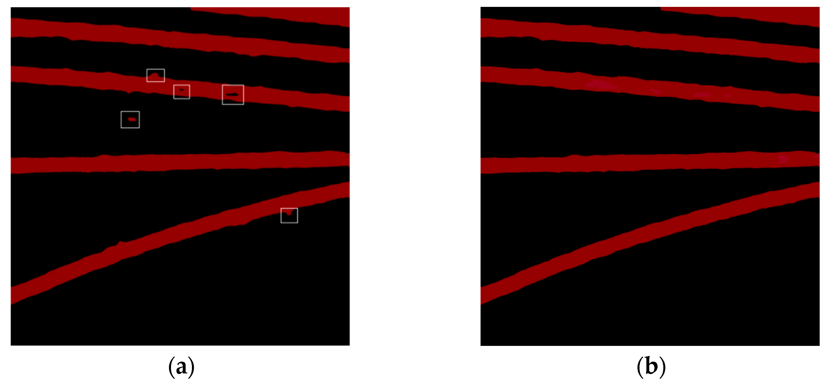
morphologyEx() function parameter set to MOP_CLOSE. Through optimization with morphological algorithms, a more complete extraction result can be achieved. Taking the Railway track segmentation dataset as an example, the comparison of results before and after morphological processing is shown in
Figure 11.
4.2.3. Railway Dataset Experiment
To compare the overall accuracy of this algorithm with other algorithms, an evaluation was conducted using the railway track segmentation dataset. The evaluation metrics and runtime of the proposed model were compared with the U-Net semantic segmentation network [
25], L-UNet network [
26], DeepLabv3 model with ResNet backbone [
27], and DeepLabv3+ network [
28] using the improved MobileNetV2 backbone network with rectangular contrast. For ease of comparison, the prediction time was selected to measure the model’s time difference, and 288 original images from the railway track segmentation dataset were used for prediction. It can be observed that the DeepLabv3+ model with the MobileNetV2 backbone network achieves improved accuracy and lower prediction time compared to the U-Net network and DeepLabv3 network. This indicates that utilizing a lightweight backbone network, such as MobileNetV2, in the DeepLabv3+ model can significantly reduce the network’s scale without compromising accuracy and overall runtime.
Furthermore, the MobileNetV3 backbone network was employed in this paper, which further enhances accuracy and reduces runtime by approximately 5% compared to MobileNetV2 before the morphological processing. Based on the above analysis, it can be concluded that the proposed method improves the accuracy of railway track extraction and significantly reduces the overall running time. The comparison results are presented in
Table 2.
Despite the improvements made in the DeepLabv3+ model, there are still some imperfections in the extracted railway track area, such as holes, bumps, and spots. This is mainly due to the nature of semantic segmentation, which operates at a pixel level. In non-railway areas of the original image, there may be pixels that are similar or identical to those in the railway area, leading to segmentation errors. To further enhance the semantic segmentation results, morphological erosion and dilation operations can be employed. The open operation (erosion followed by dilation) helps to remove spots and bumps, while the close operation (dilation followed by erosion) can eliminate voids within the railway area without altering the overall shape. The effectiveness of these morphological operations depends on adjusting the size of the kernel in the algorithm to achieve optimal results. By applying these operations to the railway area, a complete and refined railway track can be obtained.
Table 2 compares the results obtained by the model proposed in this paper and other extraction models, highlighting the improvements achieved. The comparison between the model in this paper and other model extraction results is shown in
Table 3.
4.2.4. DeepGlobe Public Data Set Model Comparative Experimental Analysis
To assess the generalization ability of the proposed model, the same experiment was conducted on the DeepGlobe public dataset, which was preprocessed to enable semantic segmentation. Different models were trained on this dataset, and predictions were made on 398 raw images. The experimental results demonstrate that similar to the results obtained on the railway track segmentation dataset, the proposed model exhibits improved extraction accuracy compared to other models and reduced computational time. The comparison results of evaluation metrics and runtime are presented in
Table 4.
The public dataset contains road environments that are more complex, and as a result, the evaluation metrics have decreased to varying degrees compared to the railway track segmentation dataset. However, under the same conditions, the proposed model still exhibits improved extraction performance compared to other models. The road images extracted by the proposed model undergo further processing using a morphological algorithm, resulting in more complete road features. A comparison between the results of the proposed model after morphological processing and other models is presented in
Table 5.
4.3. Analysis of Ablation Experiment
To verify whether the enhanced DeepLabv3+ model proposed in this paper achieves improved accuracy and reduced runtime compared to the original model, ablation experiments were conducted on both the DeepGlobe public and railway track segmentation datasets.
The ablation experiments conducted in this paper primarily focused on examining the impacts of the MobileNetV3 backbone extraction network, MobileNetV2 backbone extraction network, CARAFE, and morphological algorithm on the accuracy and runtime of railway track extraction, while keeping other conditions constant. Initially, experiments were conducted using the MobileNetV2 backbone extraction network to evaluate the effects of CARAFE and the morphological algorithm on extraction accuracy and runtime. Subsequently, the same experimental operations were performed using the MobileNetV3 backbone extraction network.
The experimental results on the railway track segmentation dataset demonstrate that replacing the upsampling module with CARAFE leads to a slight improvement in accuracy and a reduction in runtime. Furthermore, the addition of the morphological algorithm further enhances accuracy but significantly increases the runtime. However, under identical conditions, the MobileNetV3 backbone extraction network is more efficient and consumes less time than the MobileNetV2 extraction network. The comparison results of the ablation experiments on the railway track segmentation dataset are presented in
Table 6.
The experimental results on the DeepGlobe public dataset exhibit similar trends to those observed on the railway track segmentation dataset. The incorporation of CARAFE and the morphology algorithms leads to an improvement in extraction accuracy to some extent, while the performance of the MobileNetV3 backbone surpasses that of MobileNetV2. The comparison results of the ablation experiments on the DeepGlobe public dataset are presented in
Table 7.
Firstly, the results of the ablation experiments on two datasets show that MobileNetV3 achieves slightly higher accuracy than MobileNetV2 while also reducing processing time by approximately 5%. This experiment provides evidence that MobileNetV3 inherits the strengths of MobileNetV2 while incorporating “lightweight” enhancements.
Furthermore, compared to the default 16x Bilinear upsampling, employing CARAFE upsampling leads to a slight improvement in accuracy without significant differences in time consumption. This experiment demonstrates that CARAFE upsampling, which considers image semantic features and adaptive kernel selection, can effectively enhance model performance.
Finally, the composite operation of morphological algorithms can also significantly improve the extraction results.
5. Discussion
Based on the experimental results, it is evident that the proposed method has significantly enhanced the extraction accuracy while reducing time consumption. This improvement can be attributed to the utilization of NAS (Neural Architecture Search) and NetAdapt algorithms in the MobileNetV3 network. Furthermore, the inclusion of the CARAFE module and morphology algorithm has a noticeable effect on improving the extraction accuracy, albeit at the cost of increased overall running time. The CARAFE module, a lightweight upsampling operator, considers the content information of the feature map while maintaining a low parameter count. This leads to shorter upsampling time and a slight improvement in accuracy. The morphology algorithm, on the other hand, assesses the validity of a region based on the pixel distribution within a binary image. Suppose the number of pixel values surrounding a particular region significantly exceeds the number of pixel values within the region. In that case, the pixel value of the region is modified, effectively eliminating spots and holes.
To enhance the generalization capability of this paper’s model, both data and model aspects were addressed. Firstly, in terms of data, a railway segmentation dataset was created using unmanned aerial vehicle (UAV) images taken from various regions and cities in China. The dataset encompasses diverse weather conditions, terrains, and environments, including railway stations in different regions of China. After partitioning the railway segmentation dataset into training, validation, and test sets, data augmentation techniques were applied to the training set. Secondly, for the model aspect, SGD (Stochastic Gradient Descent) was chosen as the optimizer to update and compute the network parameters influencing the model training and outputs, driving them towards or achieving optimal values.
Furthermore, an L2 regularization module was incorporated into the model to prevent overfitting. During the model training process, the best weights and the final training weights were automatically saved for optional selection. To validate the model’s generalization ability in different traffic scenarios, experiments were also conducted on the publicly available DeepGlobe dataset. The experimental results demonstrate that this model is suitable for diverse environments and exhibits a certain generalization capability.


