Enhancing the Performance of a Renewable Energy System Using a Novel Predictive Control Method

Abstract

The current study concerns improving the performance of a renewable energy system using systematically designed control algorithms. The performance of the system under study is evaluated under two operating scenarios: the first in which the system consists of only a wind-driven synchronous generator connected to the utility grid; in the second scenario, the generator is combined with a photo-voltaic solar system and a battery for supplying a load. Each system component is modeled and thoroughly described. To maximize the benefits of solar and wind energies, two separate maximum power point tracking procedures are adopted. Furthermore, to enhance the generator’s dynamics, a novel predictive control scheme is designed and validated by comparing its performance with traditional predictive control. The novel predictive controller utilized a simple and unique cost function to avoid the shortages of traditional predictive controllers. For standalone operation, an effective procedure is adopted to ensure the power balance between the generation, storage, and isolated load units. To evaluate the effectiveness of the designed controllers under different operating regimes, Matlab/Simulink is utilized for this task. The obtained results confirm the superiority of the novel predictive scheme used with the synchronous generator over the classic control approach for the two operating scenarios. This has been shown in the form of reduced ripples and reduced current harmonics. The obtained results are also confirming the validity of the adopted maximum power tracking strategies with solar panels and wind turbines as well. Furthermore, balanced power delivery is achieved thanks to the adopted management strategy for standalone operation, which enhances the overall system performance.

1. Introduction

The remarkable shortage in the deposits of fossil fuels around the world inspired scientists to look for alternative sources. Renewable energy can be found in different forms according to its origin, like wind, solar, geothermal, wave, and nuclear energy [1]. However, in order to realize the maximum exploitation of those types, a precise plan should be followed in which the system emulation is fulfilled through the modeling and control of each system component. The renewable energy system also has different configurations according to the number of generation units used and the point of common coupling. For example, there are systems that consist of only one generating unit [2]. The main challenge when connecting these systems is ensuring power synchronization with the grid and delivering power with high quality. In such systems, attention must be paid to ensure appropriate dynamic performance for the generation unit and grid as well. Accordingly, the choice of adopted control with machine and grid sides must be precisely accomplished [3].

Alternatively, renewable energy systems can come in another form in which they are disconnected from the grid but feed remote, isolated loads [4]. These types can consist of only one generation unit. However, these types are not so favored due to their reduced reliability and limited generation of power [5]. Consequently, the orientation towards hybrid renewable systems is given higher attention. Higher dependability and increased load ratings are provided by hybrid systems [6,7]. In general, these systems comprise multiple generation units [8]. Additionally, due to natural weather conditions, hybrid systems are usually linked with storage devices such as batteries, fuel cells, and flywheels [9]. Accordingly, a proper power management system should be present to ensure smooth power exchange between all system components.

Present studies show the viability of combining many energy sources, and they also highlight the consequences of variations in weather conditions on hybrid systems [10]. The majority of research; however, concentrated on the scale and operational conditions of hybrid energy systems with straightforward structures. For example, various optimizers were employed in [11,12] to scale the hybrid system components. The investigation that was published in [13] examined how a hybrid system fed DC average loads while the AC category loads were considered in [14]. Although the studies in [15,16] investigated how hybrid power systems operate independently, they didn’t outline the examination of energy management approaches.

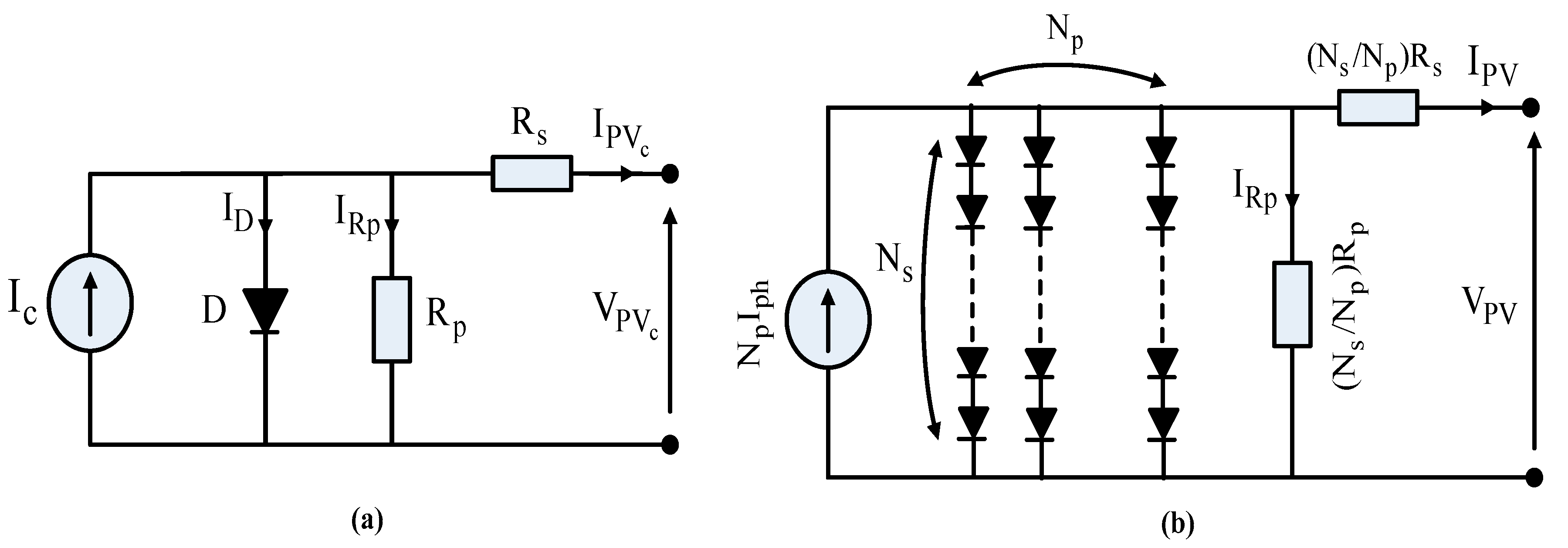
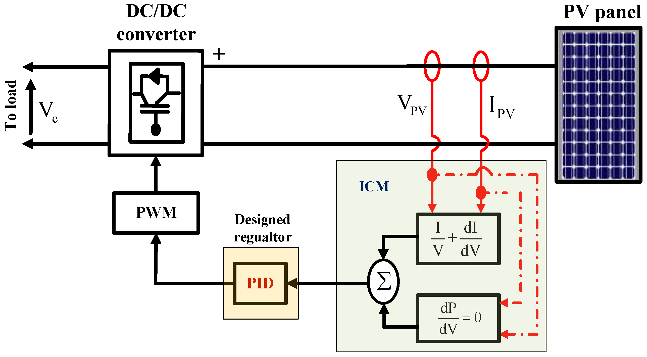
Further research on hybrid power systems can be conducted by incorporating effective power regulation and storage technologies. The target of power management (PM) is to keep a balance among the generated, consumed, and stored powers. The investigation may also take the form of developing new controllers. For example, the efficiency of the PV modules has been improved through extensive research. To highlight this issue, several techniques for monitoring the maximum power point (MPP) of a PV module have been put forth [17,18]. PV systems must incorporate an MPPT technique for the solar array because PV modules still have low conversion efficiency. The operating voltage of the array determines how much power a PV system will produce. The MPP of a PV changes with temperature and solar insulation [19]. Accordingly, the switching signals for the PV power converter should be handled to ensure the achievement of this purpose.

In wind systems, a variety of generator topologies were utilized, starting with the asynchronous generators with their different categories, such as squirrel cage or wound rotor types [20,21], and then moving forward to the synchronous generators with permanent magnets [22]. However, there is still an obvious gap in studying the performance of wind generation systems using multi-phase machines as an alternative to the traditional, previously mentioned three-phase machine types. Multi-phase machines have recently attracted new interest [23,24]. Furthermore, having a lot of phases enables power segmentation, which distributes loads across a variety of components [25]. This makes it possible to use power components with high switching frequencies, which reduces the current harmonics and the torque ripples [26,27]. These benefits shouldn’t, however, obscure how intricate their control is in both normal and impaired modes [28]. Due to the advantages of multi-phase machines, several studies have been presented to achieve the optimal performance of such machines.

The five-phase PMSG has proven itself as a superior multi-phase generator type in comparison with the multi-phase induction machines. Different control algorithms are considered for managing the performance of the five-phase PMSG. In [29], the authors adopted the vector control principle to achieve decoupled regulation of the d-q components of the generated current. A good steady-state performance was achieved; however, a delay in the response was present. Alternatively, the DTC control was used in [30], which replaced the PI current regulators with two hysteresis comparators and a unique voltage look-up table. Faster dynamics and reduced complexity were obtained with the DTC in comparison with vector control. However, the ripples of generated quantities and current harmonics were very noticeable in DTC. 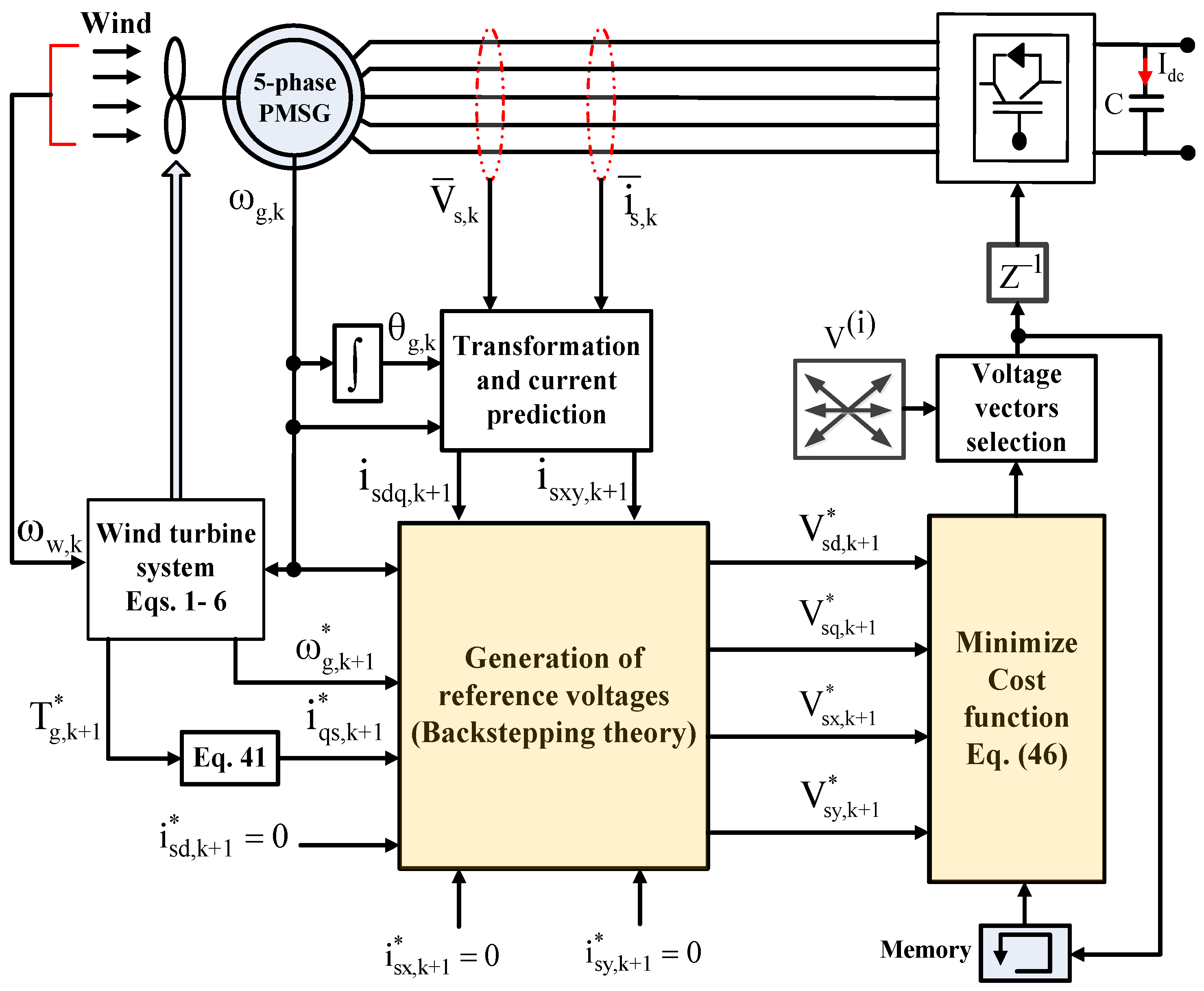After that, recent control theories such as sliding mode control (SMC) [31] were adopted for controlling the operation of the five-phase PMSG. Better performance was obtained compared with the vector control and DTC techniques. However, the use of PWM modulators with these control approaches increased the overall system complexity. This is in addition to some internal control issues, such as the chattering effect in the SMC approach. Accordingly, an effective control theory appeared and was used as an alternative to the mentioned control topologies, which is the predictive control (PC) theory [32]. This controller has the capacity to implement multiple control goals at once. It also can perform its task without utilizing a modulation scheme such as PWM. All of these facts provided more simplicity and flexibility for such a controller. The PC depends on utilizing a unique convergence condition (CC) that must be achieved to fulfill the control requirements. Based upon this hypothesis, different convergence conditions are adopted according to which variables should be controlled. For example, in [33], predictive torque control (PTC) is considered, in which the CC is expressed by a mathematical formula that incorporates the definite errors of the generator torque and flux. The control target is to minimize this CC when the actual variables deviate from their references. Better performance was achieved with the PTC compared with the classic DTC and vector control. However, the main challenge was determining the appropriate value of the weighting coefficient to be used in the CC. Any imprecise selection of this value results in deteriorating control performance due to inaccurate voltage selection. Accordingly, the need to use a CC that doesn’t use a WC and combine control variables from the same category became a requirement. The predictive current control (PCC) [34] is then adopted to fulfill these requirements, and better performance is achieved. However, the high computation burdens for the PTC and PCC were common and where not enhanced anymore. As a solution, the current paper presents the design for an effective predictive controller that avoids the deficiencies in previous controllers. The modified structure of the proposed controller helped ensure better steady state and transient operations. Additionally, it succeeded in relieving the computation capacity in relevant with the classic predictive controllers. To ensure power balance, an effective power management (PM) procedure is adopted. Furthermore, the control designs of the used converters are systematically explained.

Upon this detailed review, the paper contributions can then be outlined as follows:

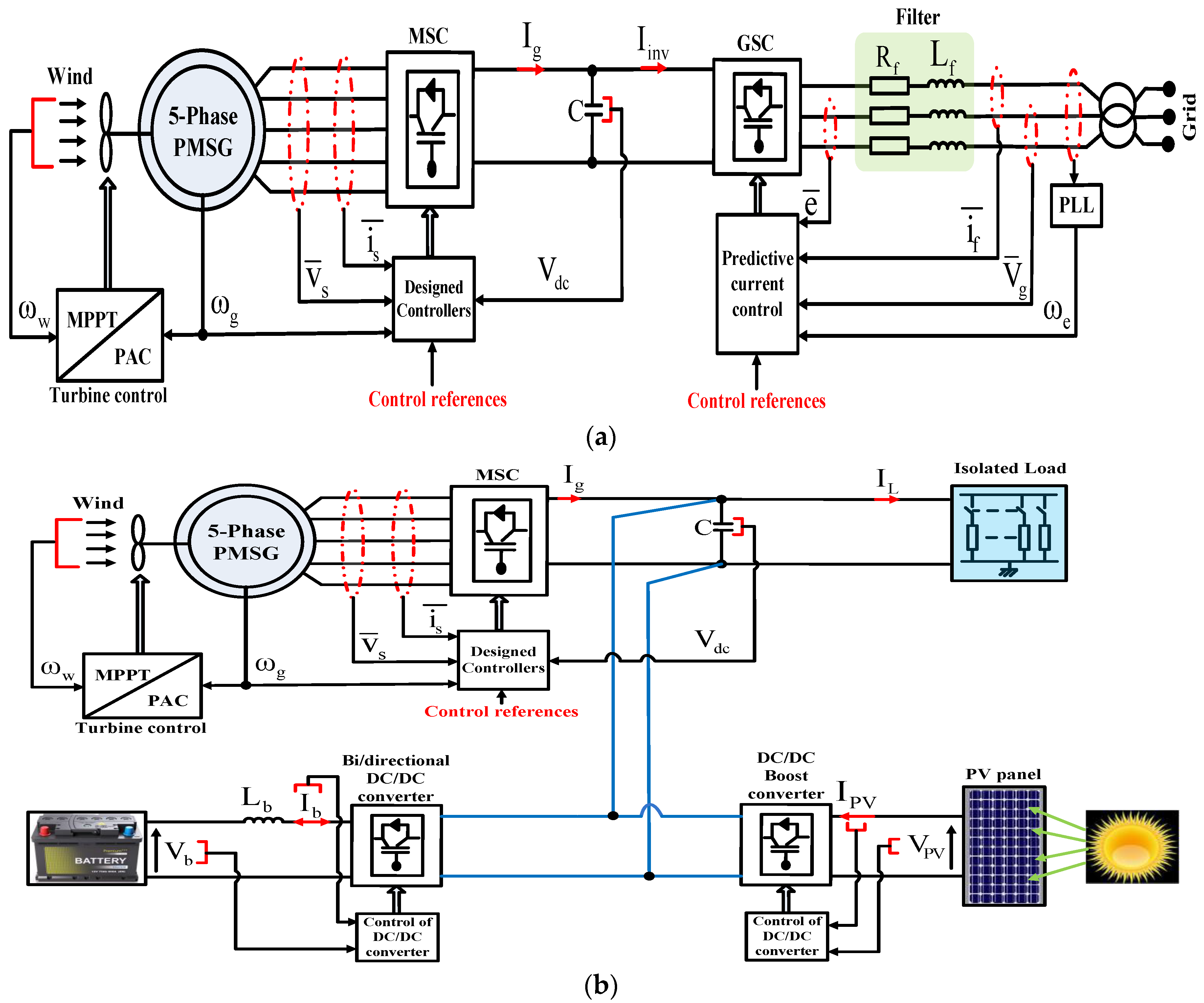
• Introducing a detailed examination of a renewable energy system operated in two different modes: grid connected and standalone.
• A detailed design for the control systems used for each system unit is discussed.
• A novel predictive control topology is developed and applied to enhance the synchronous generator’s dynamics.
• An effective MPPT strategy for the PV system is formulated and validated.
• For standalone operation, an efficient procedure is adopted to maintain the power balance.
• The feasibility of the considered generation system is confirmed for different operating conditions.

The current paper is organized as follows: in Section 2, the modeling of all system components is provided in detail. Section 3 describes the control design for all system components. Section 4 introduces and defines the procedure utilized to ensure power balance. The testing results are provided and analyzed in Section 5. Finally, Section 6 gives the study’s conclusion.

2. System under Study

The system under investigation is depicted in Figure 1. It consists of a wind generation system that incorporates a five-phase PMSG, a PV solar system, and a battery. The system, as mentioned earlier, can operate in two states: the first, in which the system is connected to the grid via a converter (GSC), which is controlled using the PCC principle (Figure 1a); and the second, in which the system is feeding an isolated load (Figure 1b). The system also includes the controllers used with all components. The control systems include the battery control system, the PV panel’s converter control system, the turbine power system, and the five-phase PMSG control system as well. Therefore, all of these units must be accurately emulated and adjusted for each particular task in order to preserve proper system operation.

2.1. Wind Power System

This system consists of the turbine and five-phase PMSG and their relevant controllers. Also, the system incorporates the machine-side converter, which needs to be controlled to manage the delivered power to either the grid or an isolated load. Accordingly, the turbine and generator modeling is presented in the following subsections.

2.1.1. Turbine Modeling

To represent the turbine’s dynamics, a numerical model is required. The MPPT is often employed to obtain the highest amount of wind energy available [35].

The wind power (${\mathrm{P}}_{\mathrm{w}})$ and turbine power (${\mathrm{P}}_{\mathrm{t}})$ are expressed by

$${\mathrm{P}}_{\mathrm{w}}=0.5{\mathsf{\rho }\mathrm{A}\mathsf{\omega }}_{\mathrm{w}}^3, {\mathrm{and} \mathrm{P}}_{\mathrm{t}}={\mathrm{C}}_{\mathrm{P}}{\mathrm{P}}_{\mathrm{w}}$$

(1)

The power coefficient ${\mathrm{C}}_{\mathrm{P}}$ can be calculated by [36]

$${\mathrm{C}}_{\mathrm{P}}\left(\mathsf{\gamma },\mathsf{\beta }\right)=\left[\frac{80}{{\mathsf{\gamma }}_{\mathrm{i}}}-0.31\mathsf{\beta }-0.0011{\mathsf{\beta }}^{2.14}-6.99\right]{\mathrm{e}}^{\left(\frac{-18.4}{{\mathsf{\gamma }}_{\mathrm{i}}}\right)}$$

(2)

Using (1,2), the turbine’s torque is evaluated as

$${\mathrm{T}}_{\mathrm{t}}=\frac{{\mathrm{P}}_{\mathrm{t}}}{{\mathsf{\omega }}_{\mathrm{t}}}=\frac{{\mathrm{C}}_{\mathrm{P}}.\left(0.5{\mathsf{\rho }\mathrm{A}\mathsf{\omega }}_{\mathrm{w}}^3\right)}{{\mathsf{\omega }}_{\mathrm{t}}}$$

(3)

The generator’s torque (${\mathrm{T}}_{\mathrm{g}})$ and speed (${\mathsf{\omega }}_{\mathrm{g}})$ can be in turn evaluated by

$${\mathrm{T}}_{\mathrm{g}}=\frac{{\mathrm{T}}_{\mathrm{t}}}{\mathrm{X}} \mathrm{and} {\mathsf{\omega }}_{\mathrm{g}}={\mathrm{X}\mathsf{\omega }}_{\mathrm{t}}$$

(4)

where X is the gear ratio.

The dynamics of the turbine/generator system are expressed by

$$\frac{{\mathrm{d}\mathsf{\omega }}_{\mathrm{t}}}{\mathrm{dt}}=\frac{{\mathrm{T}}_{\mathrm{t}}-{\mathrm{XT}}_{\mathrm{g}}-{\mathrm{fX}\mathsf{\omega }}_{\mathrm{t}}}{\left(\frac{{\mathrm{J}}_{\mathrm{t}}}{\mathrm{X}}+{\mathrm{XJ}}_{\mathrm{g}}\right)}$$

(5)

where ${\mathrm{J}}_{\mathrm{t}}$ and ${\mathrm{J}}_{\mathrm{g}}$ are the turbine and generator inertias, and f is the friction constant.

It is argued that an ideal value of ${\mathsf{\gamma }}_{\mathrm{opt}}$ must be chosen and used in order to ensure maximum ${\mathrm{C}}_{\mathrm{P},\max }$ and accordingly ${\mathrm{P}}_{\mathrm{w},\max }$ can be obtained.

Lastly, the reference speed signals to be used are calculated by

$${\mathsf{\omega }}_{\mathrm{t}}^{*}=\frac{2{\mathsf{\gamma }}_{\mathrm{opt}}{\mathsf{\omega }}_{\mathrm{w}}}{\mathrm{D}} \mathrm{and} {\mathsf{\omega }}_{\mathrm{g}}^{*}={\mathrm{X}\mathsf{\omega }}_{\mathrm{t}}^{*}$$

(6)

2.1.2. Modeling of PMSG and Machine Side Converter

The dynamics of the surface mounted five-phase PMSG can be represented using the following formulas [29,30]: defined in the rotating (d-q-x-y) synchronous frame and defined in a discrete form at instant kT_s

$$\frac{{\mathrm{di}}_{\mathrm{sd},\mathrm{k}}}{\mathrm{dt}}=\frac{1}{{\mathrm{L}}_{\mathrm{s}}}\left[{\mathrm{V}}_{\mathrm{sd},\mathrm{k}}-{\mathrm{R}}_{\mathrm{s}}{\mathrm{i}}_{\mathrm{sd},\mathrm{k}}+{\mathrm{pL}}_{\mathrm{s}}{\mathsf{\omega }}_{\mathrm{g},\mathrm{k}}{\mathrm{i}}_{\mathrm{sq},\mathrm{k}}\right]$$

$$\frac{{\mathrm{di}}_{\mathrm{sq},\mathrm{k}}}{\mathrm{dt}}=\frac{1}{{\mathrm{L}}_{\mathrm{s}}}\left[{\mathrm{V}}_{\mathrm{sq},\mathrm{k}}-{\mathrm{R}}_{\mathrm{s}}{\mathrm{i}}_{\mathrm{sq},\mathrm{k}}-{\mathrm{pL}}_{\mathrm{s}}{\mathsf{\omega }}_{\mathrm{g},\mathrm{k}}\left({\mathrm{i}}_{\mathrm{sd},\mathrm{k}}+\frac{{\mathsf{\psi }}_{\mathrm{f},\mathrm{k}}}{{\mathrm{L}}_{\mathrm{s}}}\right)\right]$$

$$\frac{{\mathrm{di}}_{\mathrm{sx},\mathrm{k}}}{\mathrm{dt}}=\frac{1}{{\mathrm{L}}_{\mathrm{l}}}{\mathrm{V}}_{\mathrm{sx},\mathrm{k}}-\frac{{\mathrm{R}}_{\mathrm{s}}}{{\mathrm{L}}_{\mathrm{l}}}{\mathrm{i}}_{\mathrm{sx},\mathrm{k}}$$

$$\frac{{\mathrm{di}}_{\mathrm{sy},\mathrm{k}}}{\mathrm{dt}}=\frac{1}{{\mathrm{L}}_{\mathrm{l}}}{\mathrm{V}}_{\mathrm{sy},\mathrm{k}}-\frac{{\mathrm{R}}_{\mathrm{s}}}{{\mathrm{L}}_{\mathrm{l}}}{\mathrm{i}}_{\mathrm{sy},\mathrm{k}}$$

(7)

where ${\mathrm{R}}_{\mathrm{s}}$, ${\mathrm{L}}_{\mathrm{s}}$ and ${\mathrm{L}}_{\mathrm{l}}$ are respectively the stator resistance, stator inductance, and stator leakage inductance. p is the pole pairs, ${\mathsf{\omega }}_{\mathrm{g}}$ is the generator mechanical speed, and ${\mathsf{\psi }}_{\mathrm{f}}$ is the rotor flux.

The mechanical dynamics of the generator can also be represented by

$$\frac{{\mathrm{d}\mathsf{\omega }}_{\mathrm{g},\mathrm{k}}}{\mathrm{dt}}=\frac{1}{{\mathrm{J}}_{\mathrm{g}}}\left({\mathrm{T}}_{\mathrm{t},\mathrm{k}}-{\mathrm{T}}_{\mathrm{g},\mathrm{k}}-{\mathrm{f}\mathsf{\omega }}_{\mathrm{g},\mathrm{k}}\right)$$

(8)

where the torque ${\mathrm{T}}_{\mathrm{g}}$ in (8) can be expressed by

$${\mathrm{T}}_{\mathrm{g},\mathrm{k}}=\frac{5}{2}\mathrm{p}\left({\mathsf{\psi }}_{\mathrm{f},\mathrm{k}}{\mathrm{i}}_{\mathrm{sq},\mathrm{k}}\right)$$

(9)

A five-phase converter can act as the handler of the generated power from the five-phase PMSG, as stated in [37]. The switching states for this converter can be represented by

$${\mathrm{S}}_{\mathrm{abcde},\mathrm{k}}={\left[\begin{array}{ccc}{\mathrm{S}}_{\mathrm{a},\mathrm{k}}& {\mathrm{S}}_{\mathrm{b},\mathrm{k}}& {\mathrm{S}}_{\mathrm{c},\mathrm{k}}\end{array}\begin{array}{cc}{ \mathrm{S}}_{\mathrm{d},\mathrm{k}}& {\mathrm{S}}_{\mathrm{e},\mathrm{k}}\end{array}\right]}^{\mathrm{T}}\in {\left\{0,1\right\}}^5$$

(10)

If ${\mathrm{S}}_{\mathrm{i}}=1$ for $\mathrm{i}\in \left\{\begin{array}{ccc}\mathrm{a}& \mathrm{b}& \mathrm{c}\end{array}\begin{array}{cc} \mathrm{d}& \mathrm{e}\end{array}\right\}$, the lower switch is turned off and the upper one is turned on. If ${\mathrm{S}}_{\mathrm{k}}=0$, on the other hand, the lower switch will be on while the top switch will be off.

Accordingly, the generator terminal voltages ${\mathrm{V}}_{\mathrm{abcde}}$ can be evaluated as follows: [38]

$$\left[\begin{array}{c}{\mathrm{V}}_{\mathrm{a},\mathrm{k}}\\ {\mathrm{V}}_{\mathrm{b},\mathrm{k}}\\ \begin{array}{c}{\mathrm{V}}_{\mathrm{c},\mathrm{k}}\\ {\mathrm{V}}_{\mathrm{d},\mathrm{k}}\\ {\mathrm{V}}_{\mathrm{e},\mathrm{k}}\end{array}\end{array}\right]=\frac{{\mathrm{V}}_{\mathrm{dc},\mathrm{k}}}{5}\left[\begin{array}{ccc}4& -1& \begin{array}{ccc}-1& -1& -1\end{array}\\ -1& 4& \begin{array}{ccc}-1& -1& -1\end{array}\\ \begin{array}{c}-1\\ -1\\ -1\end{array}& \begin{array}{c}-1\\ -1\\ -1\end{array}& \begin{array}{ccc}\begin{array}{c}4\\ -1\\ -1\end{array}& \begin{array}{c}-1\\ 4\\ -1\end{array}& \begin{array}{c}-1\\ -1\\ 4\end{array}\end{array}\end{array}\right]\left[\begin{array}{c}{\mathrm{S}}_{\mathrm{a},\mathrm{k}}\\ {\mathrm{S}}_{\mathrm{b},\mathrm{k}}\\ \begin{array}{c}{\mathrm{S}}_{\mathrm{c},\mathrm{k}}\\ {\mathrm{S}}_{\mathrm{d},\mathrm{k}}\\ {\mathrm{S}}_{\mathrm{e},\mathrm{k}}\end{array}\end{array}\right]$$

(11)

2.2. DC Bus and Filter Modeling

Under grid tied operation, the generation system is composed only of the wind-driven five-phase PMSG, with its output terminals connected to a five-phase converter (MSC). The MSC handles the power through a DC bus, and then it delivers it to the grid through a three-phase GSC. The control of GSC aims to adapt the DC bus voltage and maintain a unity PF [39,40].

Given that the grid voltage ${\overline{\mathrm{V}}}_{\mathrm{g},\mathrm{k}}$ is aligned totally along the rotating frame quadrature axis, accordingly

$${\mathrm{V}}_{\mathrm{qg},\mathrm{k}}=\left|{\overline{\mathrm{V}}}_{\mathrm{g},\mathrm{k}}\right|, {\mathrm{and} \mathrm{V}}_{\mathrm{dg},\mathrm{k}}=0.0$$

(12)

where ${\mathrm{V}}_{\mathrm{dg}}$ and ${\mathrm{V}}_{\mathrm{qg}}$ are the grid voltage components. Accordingly, the voltage distribution across the grid filter is represented by

$$\frac{{\mathrm{di}}_{\mathrm{df},\mathrm{k}}}{\mathrm{dt}}=\left({\mathrm{E}}_{\mathrm{d},\mathrm{k}}-{\mathrm{R}}_{\mathrm{f}}{\mathrm{i}}_{\mathrm{df},\mathrm{k}}+{\mathsf{\omega }}_{\mathrm{e},\mathrm{k}}{\mathrm{L}}_{\mathrm{f}}{\mathrm{i}}_{\mathrm{qf},\mathrm{k}}\right)/{\mathrm{L}}_{\mathrm{f}}$$

(13)

$$\frac{{\mathrm{di}}_{\mathrm{qf},\mathrm{k}}}{\mathrm{dt}}=\left({\mathrm{E}}_{\mathrm{q},\mathrm{k}}-{\mathrm{R}}_{\mathrm{f}}{\mathrm{i}}_{\mathrm{qf},\mathrm{k}}-{\mathsf{\omega }}_{\mathrm{e},\mathrm{k}}{\mathrm{L}}_{\mathrm{f}}{\mathrm{i}}_{\mathrm{df},\mathrm{k}}-{\mathrm{V}}_{\mathrm{qg},\mathrm{k}}\right)/{\mathrm{L}}_{\mathrm{f}}$$

(14)

where the filter’s resistance and inductance are and ${\mathrm{L}}_{\mathrm{f}}$, respectively. The GSC d-q voltages are noted as ${\mathrm{E}}_{\mathrm{d}}$ and ${\mathrm{E}}_{\mathrm{q}}$, the grid angular frequency is ${\mathsf{\omega }}_{\mathrm{e}}$, which is determined by a PLL system, and the d-q axis current components of the general utility are noted by ${\mathrm{i}}_{\mathrm{df}}$ and ${\mathrm{i}}_{\mathrm{qf}}$.

Then, the dynamic of DC bus is represented by

$$\mathrm{C}\frac{{\mathrm{dV}}_{\mathrm{dc},\mathrm{k}}}{\mathrm{dt}}={\mathrm{I}}_{\mathrm{dc},\mathrm{k}}={\mathrm{I}}_{\mathrm{g},\mathrm{k}}-{\mathrm{I}}_{\mathrm{inv},\mathrm{k}}$$

(15)

where C is bus capacitance, ${\mathrm{V}}_{\mathrm{dc}}$ is the DC potential, ${\mathrm{I}}_{\mathrm{dc}}$ is the current through DC link, ${\mathrm{I}}_{\mathrm{g}}$ is the generated current and ${\mathrm{I}}_{\mathrm{inv}}$ is the input current to the GSC.

2.3. PV and Battery Systems Modeling

2.3.1. Modeling of PV System

The second operation scenario for the system is the standalone operation, in which the wind generation system is combined with a PV system and a battery while supplying an island load. Accordingly, the modeling of PV and battery units should be derived.

In a solar cell, solar energy is converted into electrical energy using the photovoltaic phenomenon. A solar cell’s circuit is shown in Figure 2a [41].

$N_p$ parallel PV threads with $N_s$ PV cells wired in series make up an array. To provide the required load power, a combination of series/parallel attached cells and panels is considered. The PV array’s circuit is illustrated in Figure 2b.

The current ${\mathrm{I}}_{{\mathrm{PV}}_{\mathrm{c}}}$ is computed by [42].

$${\mathrm{I}}_{{\mathrm{PV}}_{\mathrm{c}},\mathrm{k}}={\mathrm{I}}_{\mathrm{c},\mathrm{k}}-{\mathrm{I}}_{\mathrm{D},\mathrm{k}}-{\mathrm{I}}_{{\mathrm{R}}_{\mathrm{p}},\mathrm{k}}={\mathrm{I}}_{\mathrm{c},\mathrm{k}}-{\mathrm{I}}_{\mathrm{o},\mathrm{k}}\left[{\mathrm{e}}^{\left(\mathrm{q}.\frac{{\mathrm{V}}_{{\mathrm{PV}}_{\mathrm{c}},\mathrm{k}}+{\mathrm{R}}_{\mathrm{s}}{\mathrm{I}}_{{\mathrm{PV}}_{\mathrm{c}},\mathrm{k}}}{\nabla \mathrm{BT}}\right)}-1\right]-\frac{{\mathrm{V}}_{{\mathrm{PV}}_{\mathrm{c}},\mathrm{k}}+{\mathrm{R}}_{\mathrm{s}}{\mathrm{I}}_{{\mathrm{PV}}_{\mathrm{c}},\mathrm{k}}}{{\mathrm{R}}_{\mathrm{p}}}$$

(16)

where ${\mathrm{I}}_{\mathrm{c}}$ is the source direct current, ${\mathrm{I}}_{\mathrm{o}}$ is the reverse current, ${\mathrm{I}}_{\mathrm{D}}$ is the diode current, ${\mathrm{I}}_{{\mathrm{R}}_{\mathrm{P}}}$ is the current through parallel resistance, $\nabla$ is ideality factor, T is the temperature in Kelvin, B is the constant of Boltzman, and ${\mathrm{V}}_{{\mathrm{PV}}_{\mathrm{c}}}$ is the cell voltage.

The source direct current ${\mathrm{I}}_{\mathrm{c}}$ is then expressed by

$${\mathrm{I}}_{\mathrm{c},\mathrm{k}}=\left[{\mathrm{I}}_{\mathrm{sc},\mathrm{k}}+0.001{\mathrm{T}}_{\mathrm{c}}\left(\mathrm{T}-298\right).{\mathrm{S}}_{\mathrm{r},\mathrm{k}}\right]$$

(17)

where ${\mathrm{I}}_{\mathrm{sc}}$ is the short-circuit cell current, ${\mathrm{T}}_{\mathrm{c}}$ is the temperature constant (A/K), and ${\mathrm{S}}_{\mathrm{r}}$ is the irradiation (W/m²).

By constructing a combination of PV cells, a PV array can be obtained that provides a current ${\mathrm{I}}_{{\mathrm{PV}}_{\mathrm{c}}}$ that can be computed by

$${\mathrm{I}}_{\mathrm{PV},\mathrm{k}}={\mathrm{N}}_{\mathrm{p}}.{\mathrm{I}}_{\mathrm{c},\mathrm{k}}-{\mathrm{N}}_{\mathrm{p}}{\mathrm{I}}_{\mathrm{o},\mathrm{k}}\left[{\mathrm{e}}^{\left(\mathrm{q}.\frac{{\mathrm{V}}_{\mathrm{PV},\mathrm{k}}+\frac{{\mathrm{N}}_{\mathrm{S}}}{{\mathrm{N}}_{\mathrm{p}}}{\mathrm{R}}_{\mathrm{s}}{\mathrm{I}}_{\mathrm{PV},\mathrm{k}}}{{\mathrm{N}}_{\mathrm{p}}{\mathrm{N}}_{\mathrm{S}}\nabla \mathrm{BT}}\right)}-1\right]-\frac{{\mathrm{V}}_{\mathrm{PV},\mathrm{k}}+\frac{{\mathrm{N}}_{\mathrm{S}}}{{\mathrm{N}}_{\mathrm{p}}}{\mathrm{R}}_{\mathrm{s}}{\mathrm{I}}_{\mathrm{PV},\mathrm{k}}}{\frac{{\mathrm{N}}_{\mathrm{S}}}{{\mathrm{N}}_{\mathrm{p}}}{\mathrm{R}}_{\mathrm{p}}}$$

(18)

Then, the developed power is given by

$${\mathrm{P}}_{\mathrm{PV},\mathrm{k}}={\mathrm{V}}_{\mathrm{PV},\mathrm{k}}.{\mathrm{I}}_{\mathrm{PV},\mathrm{k}}$$

(19)

2.3.2. Battery Model

A power storage unit is essential to cover the power reduction during harsh weather conditions due to the discontinuous wind speeds and low irradiation levels. Accordingly, the equivalent battery circuit is illustrated in Figure 3. where the variables ${\mathrm{V}}_{\mathrm{b}}$ and ${\mathrm{I}}_{\mathrm{b}}$ pertain to the voltage and current of the battery, ${\mathrm{I}}_{\mathrm{bu}}$ and ${\mathrm{I}}_{\mathrm{su}}$ to the bulk and surface currents, ${\mathrm{R}}_{\mathrm{t}}$, ${\mathrm{R}}_{\mathrm{e}}$ and ${\mathrm{R}}_{\mathrm{su}}$ to the terminal, end, and surface resistances, and ${\mathrm{C}}_{\mathrm{su}}$ and ${\mathrm{C}}_{\mathrm{bu}}$ to the surface and bulk capacitances, respectively [43].

The battery voltage equations are expressed by

$${\mathrm{V}}_{\mathrm{b},\mathrm{k}}={\mathrm{I}}_{\mathrm{b},\mathrm{k}}{\mathrm{R}}_{\mathrm{t}}+{\mathrm{I}}_{\mathrm{su},\mathrm{k}}{\mathrm{R}}_{\mathrm{su}}+{\mathrm{V}}_{\mathrm{su},\mathrm{k}}={\mathrm{I}}_{\mathrm{b},\mathrm{k}}{\mathrm{R}}_{\mathrm{t}}+{\mathrm{I}}_{\mathrm{bu},\mathrm{k}}{\mathrm{R}}_{\mathrm{e}}+{\mathrm{V}}_{\mathrm{bu},\mathrm{k}}$$

(20)

3. Design of Control Systems

This section presents and describes the specific design processes for control systems. At first, the control of the PV boost converter is explained. Then, the battery converter’s control system, the classic PTC control, and the proposed predictive control algorithm are explained.

3.1. Battery Converter Control

A bi-directional converter must be used to manage the battery operation. A view of the battery storing system is illustrated in Figure 4. A converter’s continuous model is used, through which the modulated voltage (${\mathrm{V}}_{\mathrm{m},\mathrm{bat}}$) and current (${\mathrm{I}}_{\mathrm{m},\mathrm{bat}}$) of the battery are represented by

$${\mathrm{V}}_{\mathrm{m},\mathrm{bat},\mathrm{k}}={\mathrm{m}}_{\mathrm{bat},\mathrm{k}}^{*}{\mathrm{V}}_{\mathrm{dc},\mathrm{k}}, \mathrm{and} {\mathrm{I}}_{\mathrm{m},\mathrm{bat},\mathrm{k}}={\mathrm{m}}_{\mathrm{bat},\mathrm{k}}^{*}{\mathrm{I}}_{\mathrm{bat},\mathrm{k}}$$

(21)

To produce the reference index ${\mathrm{m}}_{\mathrm{bat},\mathrm{k}}^{*}$, the reference battery voltage must first be obtained, and to do this, a PID controller is designed systematically as follows:

As indicated in Figure 4, the output of the PID regulator (ε) can be represented by

$$\mathsf{\epsilon }\left(\mathrm{s}\right)={\mathrm{V}}_{\mathrm{bat}}\left(\mathrm{s}\right)-{\mathrm{V}}_{\mathrm{m},\mathrm{bat}}^{*}\left(\mathrm{s}\right)={\mathrm{V}}_{\mathrm{bat}}\left(\mathrm{s}\right)-{\mathrm{m}}_{\mathrm{bat}}^{*}{\mathrm{V}}_{\mathrm{dc}}\left(\mathrm{s}\right)$$

(22)

In (22), the voltage difference is equivalent to the voltage through the battery inductor ${\mathrm{L}}_{\mathrm{bat}}$; accordingly

$$\mathsf{\epsilon }\left(\mathrm{s}\right)={\mathrm{sL}}_{\mathrm{bat}}{\mathrm{I}}_{\mathrm{bat}}\left(\mathrm{s}\right)$$

(23)

Utilizing (22), the dynamics of the PID-based closed loop illustrated in Figure 4 can be defined by

$$\left({\mathrm{I}}_{\mathrm{bat}}\left(\mathrm{s}\right)-{\mathrm{I}}_{\mathrm{bat}}^{*}\left(\mathrm{s}\right)\right)\ast \left(\frac{{\mathrm{K}}_{\mathrm{d},\mathrm{B}}{\mathrm{s}}^2+{\mathrm{K}}_{\mathrm{p},\mathrm{B}}\mathrm{s}+{\mathrm{K}}_{\mathrm{i},\mathrm{B}}}{\mathrm{s}}\right)={\mathrm{sL}}_{\mathrm{bat}}{\mathrm{I}}_{\mathrm{bat}}\left(\mathrm{s}\right)$$

(24)

The reference ${\mathrm{I}}_{\mathrm{bat}}^{*}$ is obtained by dividing the power difference by the voltage, as shown in Figure 4. By dividing (24) on ${\mathrm{I}}_{\mathrm{bat}}^{*}\left(\mathrm{s}\right)$ and carrying out some mathematical calculations, the transfer function (tf) that outlines the PID dynamics is represented by

$$\mathrm{Y}\left(\mathrm{s}\right)=\frac{{\mathrm{I}}_{\mathrm{bat}}\left(\mathrm{s}\right)}{{\mathrm{I}}_{\mathrm{bat}}^{*}\left(\mathrm{s}\right)}=\frac{{\mathrm{K}}_{\mathrm{d},\mathrm{B}}{\mathrm{s}}^2+{\mathrm{K}}_{\mathrm{p},\mathrm{B}}\mathrm{s}+{\mathrm{K}}_{\mathrm{i},\mathrm{B}}}{\left({\mathrm{L}}_{\mathrm{bat}}+{\mathrm{K}}_{\mathrm{d},\mathrm{B}}\right){\mathrm{s}}^2+{\mathrm{K}}_{\mathrm{p},\mathrm{B}}\mathrm{s}+{\mathrm{K}}_{\mathrm{i},\mathrm{B}}}$$

(25)

To ensure system stability, the denominator of (25) should have negative real roots. Accordingly, the next level of equality must be present

$$\left({\mathrm{L}}_{\mathrm{bat}}+{\mathrm{K}}_{\mathrm{d},\mathrm{B}}\right){\mathrm{s}}^2+{\mathrm{K}}_{\mathrm{p},\mathrm{B}}\mathrm{s}+{\mathrm{K}}_{\mathrm{i},\mathrm{B}}=0$$

(26)

Instead, the second-order dynamic system can be described using the next relationship

$${\mathrm{s}}^2+2{\mathsf{\zeta }\mathsf{\omega }}_{\mathrm{o}}\mathrm{s}+{\mathsf{\omega }}_{\mathrm{o}}^2=0$$

(27)

where $\mathsf{\zeta }$ and ${\mathsf{\omega }}_{\mathrm{o}}$ are the damping factor and natural system frequency, respectively.

By comparing (26) and (27), the values of PID coefficients are calculated as follows:

$${\mathrm{K}}_{\mathrm{d},\mathrm{B}}=1-{\mathrm{L}}_{\mathrm{bat}}, {\mathrm{K}}_{\mathrm{p},\mathrm{B}}=2{\mathsf{\zeta }\mathsf{\omega }}_{\mathrm{n}}, {\mathrm{K}}_{\mathrm{i},\mathrm{B}}={\mathsf{\omega }}_{\mathrm{n}}^2$$

(28)

3.2. Control Algorithm for PV System

As a simplified and effective solution at the same time, an incremental conductance algorithm (ICA) integrated with a PID controller is utilized for providing the optimal duty cycle, as illustrated in Figure 5. By comparing the incremental and instantaneous conductance of the PV array, the ICA follows the MPP. The tracking method is articulated on the observation that the slope tangent of the property power/voltage (P-V) in MPP is equal to zero.

This slope’s computation is provided by [44,45]:

$$\frac{{\mathrm{dP}}_{\mathrm{PV}}}{{\mathrm{dV}}_{\mathrm{PV}}}=\frac{\mathrm{d}\left({\mathrm{V}}_{\mathrm{PV}}.{\mathrm{I}}_{\mathrm{PV}}\right)}{{\mathrm{dV}}_{\mathrm{PV}}}={\mathrm{I}}_{\mathrm{PV}}+{\mathrm{V}}_{\mathrm{PV}}\frac{{\mathrm{dI}}_{\mathrm{PV}}}{{\mathrm{dV}}_{\mathrm{PV}}}$$

(29)

$$\frac{{\mathrm{I}}_{\mathrm{PV}}}{{\mathrm{V}}_{\mathrm{PV}}}+\frac{\mathrm{dI}}{{\mathrm{dV}}_{\mathrm{PV}}}=0$$

(30)

The PID regulator in the proposed tracking system receives the calculated value of (30) as an error signal and starts to minimize in favor of reducing the error between the PV slope and reference value. After that, the PID starts to provide the reference signal to the PWM generator to finally provide the switching signals to the converter IGBT.

The transfer function of a closed loop system using a PID regulator can be represented by

$$\mathrm{G}\left(\mathrm{s}\right)=\frac{{\mathrm{G}}_{\mathrm{c}}\left(\mathrm{s}\right){\ast \mathrm{G}}_{\mathrm{PID}}\left(\mathrm{s}\right)}{1+{\mathrm{G}}_{\mathrm{c}}\left(\mathrm{s}\right){\ast \mathrm{G}}_{\mathrm{PID}}\left(\mathrm{s}\right)}$$

(31)

where ${\mathrm{G}}_{\mathrm{PID}}\left(\mathrm{s}\right)$ is the representation of PID dynamics in the s-domain and can be represented by

$${\mathrm{G}}_{\mathrm{PID}}\left(\mathrm{s}\right)=\frac{{\mathrm{K}}_{\mathrm{D}}{\mathrm{s}}^2+{\mathrm{K}}_{\mathrm{P}}\mathrm{s}+{\mathrm{K}}_{\mathrm{I}}}{\mathrm{s}}$$

(32)

Alternatively, the ${\mathrm{G}}_{\mathrm{c}}\left(\mathrm{s}\right)$ is the control object (output converter voltage) transfer function, which is defined by

$${\mathrm{G}}_{\mathrm{c}}\left(\mathrm{s}\right)=\frac{1}{\mathrm{s}}$$

(33)

Then, by substituting (32) and (33) into (31), the closed-loop control is represented by

$$\mathrm{G}\left(\mathrm{s}\right)=\frac{{\mathrm{K}}_{\mathrm{D}}{\mathrm{s}}^2+{\mathrm{K}}_{\mathrm{P}}\mathrm{s}+{\mathrm{K}}_{\mathrm{I}}}{({\mathrm{K}}_{\mathrm{D}}+1){\mathrm{s}}^2+{\mathrm{K}}_{\mathrm{P}}\mathrm{s}+{\mathrm{K}}_{\mathrm{I}}}$$

(34)

The denominator of (34) represents the characteristic equation of the closed loop control based on a PID controller, which should be compared with the characteristic equation of the transfer function that contemplates the duty cycle as an input and the converter voltage as an output and which can be expressed by

$$\mathrm{H}\left(\mathrm{s}\right)=\frac{\left(1-\mathrm{D}\right){\mathrm{V}}_{\mathrm{c}}\left(\mathrm{s}\right)-{\mathrm{L}}_{\mathrm{c}}{\mathrm{I}}_{\mathrm{l}}\left(\mathrm{s}\right)\ast \mathrm{s}}{{\mathrm{L}}_{\mathrm{c}}{\mathrm{C}}_{\mathrm{c}}{\mathrm{s}}^2+\left({\mathrm{L}}_{\mathrm{c}}/{\mathrm{R}}_{\mathrm{l}}\right)\mathrm{s}+{\left(1-\mathrm{D}\right)}^2}$$

(35)

where D is the duty ratio, ${\mathrm{V}}_{\mathrm{c}}$ is the converter output voltage, ${\mathrm{L}}_{\mathrm{c}}$ and ${\mathrm{C}}_{\mathrm{c}}$ are the specified inductance and capacitance of the converter, ${\mathrm{I}}_{\mathrm{l}}$ is the current passing through the converter inductance, and ${\mathrm{R}}_{\mathrm{l}}$ is the load resistance connected to the converter terminals.

Now, by comparing the denominators of (34) and (35), the PID coefficients to be utilized are given by

$${\mathrm{K}}_{\mathrm{P}}=\frac{{\mathrm{L}}_{\mathrm{c}}}{{\mathrm{R}}_{\mathrm{l}}}, {\mathrm{K}}_{\mathrm{I}}={\left(1-\mathrm{D}\right)}^2 \mathrm{and} {\mathrm{K}}_{\mathrm{D}}={\mathrm{L}}_{\mathrm{c}}{\mathrm{C}}_{\mathrm{c}}$$

(36)

3.3. Control of GSC

The control of GSC is concerned with maintaining unity pf at the grid terminals. A predictive current scheme (PCC) is utilized for this purpose. The PCC employs a cost function that aims to limit the current deviation. The cost function can then be expressed by [46,47]

$${\Delta }_{\mathrm{k}+1}^{\mathrm{j}}={\left|{\mathrm{i}}_{\mathrm{df},\mathrm{k}+1}^{*}-{\tilde{\mathrm{i}}}_{\mathrm{df},\mathrm{k}+1}\right|}^{\mathrm{j}}+{\left|{\mathrm{i}}_{\mathrm{qf},\mathrm{k}+1}^{*}-{\tilde{\mathrm{i}}}_{\mathrm{qf},\mathrm{k}+1}\right|}^{\mathrm{j}}$$

(37)

where j is the index, and ${\tilde{\mathrm{i}}}_{\mathrm{df},\mathrm{k}+1}$ and ${\tilde{\mathrm{i}}}_{\mathrm{qf},\mathrm{k}+1}$ are the filtered signals of grid currents are calculated via utilizing (13) and (14) as follows:

$${\tilde{\mathrm{i}}}_{\mathrm{df},\mathrm{k}+1}=\left(\frac{{\mathrm{di}}_{\mathrm{df},\mathrm{k}}}{\mathrm{dt}}\right){\mathrm{T}}_{\mathrm{s}}+{\mathrm{i}}_{\mathrm{df},\mathrm{k}}, \mathrm{and} {\tilde{\mathrm{i}}}_{\mathrm{qf},\mathrm{k}+1}=\left(\frac{{\mathrm{di}}_{\mathrm{qf},\mathrm{k}}}{\mathrm{dt}}\right){\mathrm{T}}_{\mathrm{s}}+{\mathrm{i}}_{\mathrm{qf},\mathrm{k}}$$

(38)

The reference ${\mathrm{i}}_{\mathrm{qf},\mathrm{k}+1}^{*}$ is derived while adopting a grid voltage orientation along the quadrature axis of the synchronous frame by managing the error between the measured and reference values of DC bus voltage, whereas the current ${\mathrm{i}}_{\mathrm{df},\mathrm{k}+1}^{*}$ is obtained from the reactive power reference signal ${\mathrm{Q}}_{\mathrm{g},\mathrm{k}+1}^{*}$ that is kept to zero to maintain the unity pf running.

3.4. Control of Five-Phase PMSG

3.4.1. Classic Predictive Torque Control

The controlled variables taken into account by the PTC technique are torque and flux [34]. Consequently, the absolute errors and a weighting factor make up the convergence condition (CC) used by the PTC approach. The utilization of this CC offers an alternative operator to the hysteresis regulators that were previously used in classic DTC. Based upon these hypotheses, the CC formula of the PTC can be represented by

$${\mathsf{\delta }}_{\mathrm{k}+1}^{\mathrm{i}}={\left|{\mathrm{T}}_{\mathrm{g},\mathrm{k}+1}^{*}-{\tilde{\mathrm{T}}}_{\mathrm{g},\mathrm{k}+1}\right|}^{\mathrm{i}}+{\mathrm{w}}_{\mathrm{f}}{\left|{\mathsf{\psi }}_{\mathrm{g},\mathrm{k}+1}^{*}-{\tilde{\mathsf{\psi }}}_{\mathrm{g},\mathrm{k}+1}\right|}^{\mathrm{i}}$$

(39)

where ${\mathrm{T}}_{\mathrm{g},\mathrm{k}+1}^{*}$ and ${\mathsf{\psi }}_{\mathrm{g},\mathrm{k}+1}^{*}$ are the references.

The turbine system modeled using (1–6) provides the torque reference ${\mathrm{T}}_{\mathrm{g},\mathrm{k}+1}^{*}$, and the flux reference ${\mathsf{\psi }}_{\mathrm{g},\mathrm{k}+1}^{*}$ is determined as follows:

$${\mathsf{\psi }}_{\mathrm{g},\mathrm{k}+1}^{*}=\sqrt{{\left({\mathrm{L}}_{\mathrm{s}}\stackrel{0.0}{\overbrace{{\mathrm{i}}_{\mathrm{sd},\mathrm{k}+1}^{*}}}+{\mathsf{\psi }}_{\mathrm{f},\mathrm{k}+1}\right)}^2+{\left({\mathrm{L}}_{\mathrm{s}}{\mathrm{i}}_{\mathrm{sq},\mathrm{k}+1}^{*}\right)}^2+{\left({\mathrm{L}}_{\mathrm{l}}\stackrel{0.0}{\overbrace{{\mathrm{i}}_{\mathrm{sx},\mathrm{k}+1}^{*}}}\right)}^2+{\left({\mathrm{L}}_{\mathrm{l}}\stackrel{0.0}{\overbrace{{\mathrm{i}}_{\mathrm{sy},\mathrm{k}+1}^{*}}}\right)}^2}$$

(40)

The reference current ${\mathrm{i}}_{\mathrm{sq},\mathrm{k}+1}^{*}$ in (40) is evaluated by

$${\mathrm{i}}_{\mathrm{sq},\mathrm{k}+1}^{*}=\frac{{\mathrm{T}}_{\mathrm{g},\mathrm{k}+1}^{*}}{2.5{\mathrm{p}\mathsf{\psi }}_{\mathrm{f},\mathrm{k}+1}}$$

(41)

Additionally, the actual predicted signals in (39) are obtained as

$${\tilde{\mathrm{T}}}_{\mathrm{g},\mathrm{k}+1}=2.5{\mathrm{p}\mathsf{\psi }}_{\mathrm{f},\mathrm{k}+1}{\tilde{\mathrm{i}}}_{\mathrm{sq},\mathrm{k}+1}$$

(42)

$${\tilde{\mathsf{\psi }}}_{\mathrm{g},\mathrm{k}+1}=\sqrt{{\left({\mathrm{L}}_{\mathrm{s}}{\tilde{\mathrm{i}}}_{\mathrm{sd},\mathrm{k}+1}+{\mathsf{\psi }}_{\mathrm{f},\mathrm{k}+1}\right)}^2+{\left({\mathrm{L}}_{\mathrm{s}}{\tilde{\mathrm{i}}}_{\mathrm{sq},\mathrm{k}+1}\right)}^2+{\left({\mathrm{L}}_{\mathrm{l}}{\tilde{\mathrm{i}}}_{\mathrm{sx},\mathrm{k}+1}\right)}^2+{\left({\mathrm{L}}_{\mathrm{l}}{\tilde{\mathrm{i}}}_{\mathrm{syk}+1}\right)}^2}$$

(43)

The currents in (43) are evaluated with the help of (7).

The control begins by doing the calculation of (39) using the thirty two voltages that are accessible while using the FCS technique to select the vectors. It then selects and applies the principal vector that keeps the (39) at its lowest value. To predict the torque and flux (${\tilde{\mathrm{T}}}_{\mathrm{g},\mathrm{k}+1}$ and ${\tilde{\mathsf{\psi }}}_{\mathrm{g},\mathrm{k}+1}$), the control system first senses the stator voltage ${\overline{\mathrm{V}}}_{\mathrm{s}}$ and current ${\overline{\mathrm{V}}}_{\mathrm{s}}$ and uses these along with speed ${\mathsf{\omega }}_{\mathrm{g}}$. The used CC block in the scheme, which supplies the control signals to the converter, receives the reference signals ${\mathsf{\psi }}_{\mathrm{g},\mathrm{k}+1}^{*}$ and ${\mathrm{T}}_{\mathrm{g},\mathrm{k}+1}^{*}$ as inputs from the control system.

3.4.2. Predictive Flux Control

The predictive flux control (PFC) theory has been designed and applied to solve some of the classic PTC approaches for synchronous generators [48]. This has been fulfilled in the form of the convergence condition (CC). The formulated CC consisted of two similar parts, which are the absolute errors between the reference (${\mathsf{\psi }}_{\mathsf{\alpha }\mathrm{g},\mathrm{k}+1}^{*}$, ${\mathsf{\psi }}_{\mathsf{\beta }\mathrm{g},\mathrm{k}+1}^{*}$, ${\mathsf{\psi }}_{\mathrm{zg},\mathrm{k}+1}^{*}$, ${\mathsf{\psi }}_{\mathrm{wg},\mathrm{k}+1}^{*}$) and predicted values (${\mathsf{\psi }}_{\mathsf{\alpha }\mathrm{g},\mathrm{k}+1}$,${ \mathsf{\psi }}_{\mathsf{\beta }\mathrm{g},\mathrm{k}+1}$,${ \mathsf{\psi }}_{\mathrm{zg},\mathrm{k}+1}$, ${\mathsf{\psi }}_{\mathrm{wg},\mathrm{k}+1}$) of α-β-z-w components of stator flux. This helped eliminate the use of the weighting factor used by the PTC. However, the issue of using estimated variables in the CC still exists and will be handled later by the newly designed predictive controller.

The CC of the PFC can be then expressed by

$${\Lambda }_{\mathrm{k}+1}^{\mathrm{i}}={\left|{\mathsf{\psi }}_{\mathsf{\alpha }\mathrm{g},\mathrm{k}+1}^{*}-{\mathsf{\psi }}_{\mathsf{\alpha }\mathrm{g},\mathrm{k}+1}\right|}^{\mathrm{i}}+{\left|{\mathsf{\psi }}_{\mathsf{\beta }\mathrm{g},\mathrm{k}+1}^{*}-{\mathsf{\psi }}_{\mathsf{\beta }\mathrm{g},\mathrm{k}+1}\right|}^{\mathrm{i}}+{\left|{\mathsf{\psi }}_{\mathrm{zg},\mathrm{k}+1}^{*}-{\mathsf{\psi }}_{\mathrm{zg},\mathrm{k}+1}\right|}^{\mathrm{i}}+{\left|{\mathsf{\psi }}_{\mathrm{wg},\mathrm{k}+1}^{*}-{\mathsf{\psi }}_{\mathrm{wg},\mathrm{k}+1}\right|}^{\mathrm{i}}$$

(44)

By expressing the generator model in the stator frame, the flux references (${\mathsf{\psi }}_{\mathsf{\alpha }\mathrm{g},\mathrm{k}+1}^{*}$, ${\mathsf{\psi }}_{\mathsf{\beta }\mathrm{g},\mathrm{k}+1}^{*}$, ${\mathsf{\psi }}_{\mathrm{zg},\mathrm{k}+1}^{*}$, ${\mathsf{\psi }}_{\mathrm{wg},\mathrm{k}+1}^{*}$) in (44) can be evaluted using the reference flux $\left|{\mathsf{\psi }}_{\mathrm{g},\mathrm{k}+1}^{*}\right|$, the torque angle ${\mathsf{\delta }}_{\mathrm{k}+1}^{*}$ and the rotor position ${\mathsf{\theta }}_{\mathrm{g},\mathrm{k}}$.

The α-β reference flux components can be derived with the help of the reference load angle that can be expressed by [48]:

$${\mathsf{\delta }}_{\mathrm{k}+1}^{*}={\sin }^{-1}\left(\frac{{\mathrm{T}}_{\mathrm{g},\mathrm{k}+1}^{*}}{2.5\frac{\mathrm{p}}{{\mathrm{L}}_{\mathrm{s}}}\left|{\overline{\mathrm{V}}}_{\mathrm{g},\mathrm{k}+1}^{*}\right|{\mathsf{\psi }}_{\mathrm{f},\mathrm{k}+1}}\right)$$

(45)

Alternatively, the predicted actual flux components (${\mathsf{\psi }}_{\mathsf{\alpha }\mathrm{g},\mathrm{k}+1}$,${ \mathsf{\psi }}_{\mathsf{\beta }\mathrm{g},\mathrm{k}+1}$,${ \mathsf{\psi }}_{\mathrm{zg},\mathrm{k}+1}$, ${\mathsf{\psi }}_{\mathrm{wg},\mathrm{k}+1}$) can be evaluated using the generator model in (7) expressed in the stator frame. Finally, the PFC starts to evaluate (44) and determines the optimal vector that minimizes it and applies it to the terminals of the MSC.

3.4.3. New Designed Predictive Control Technique

The new control topology is designed to overcome the disadvantages of the PTC and PFC schemes. The designed controller employs a CC made up of two identical components, which eliminates the weighting coefficient and consequently helps limit the oscillations that can be brought on by inaccurate selection. Furthermore, the designed CC uses a variable that doesn’t require a lot of processing, in contrast to the variables used in PTC, such as torque and flux, and in PFC, such as flux components. This contributes to more effective control structure simplification and enhanced dynamic behavior.

The formulated controller’s CC comprises the stator voltage errors. Thus, it is expressed by

$${\complement }_{\mathrm{k}+1}^{\mathrm{i}}={\left|{\mathrm{V}}_{\mathrm{sd},\mathrm{k}+1}^{*}-{\mathrm{V}}_{\mathrm{sd},\mathrm{k}+1}\right|}^{\mathrm{i}}+{\left|{\mathrm{V}}_{\mathrm{sq},\mathrm{k}+1}^{*}-{\mathrm{V}}_{\mathrm{sq},\mathrm{k}+1}\right|}^{\mathrm{i}}+{\left|{\mathrm{V}}_{\mathrm{sx},\mathrm{k}+1}^{*}-{\mathrm{V}}_{\mathrm{sx},\mathrm{k}+1}\right|}^{\mathrm{i}}+{\left|{\mathrm{V}}_{\mathrm{sy},\mathrm{k}+1}^{*}-{\mathrm{V}}_{\mathrm{sy},\mathrm{k}+1}\right|}^{\mathrm{i}}$$

(46)

By checking (46), it is realized that all used variables are of a unique type (voltage signal). The actual voltage components (${\mathrm{V}}_{\mathrm{sd},\mathrm{k}+1}$,${\mathrm{V}}_{\mathrm{sq},\mathrm{k}+1}$,${\mathrm{V}}_{\mathrm{sx},\mathrm{k}+1}$,${\mathrm{V}}_{\mathrm{sy},\mathrm{k}+1}$) are obtained directly from the switching states of the converter with the help of the FCS principle, which selects from definite number of voltage vectors; accordingly, there is no need for high calculation capacity. On the other hand, the reference voltage signals ${\mathrm{V}}_{\mathrm{sd},\mathrm{k}+1}^{*}$, ${\mathrm{V}}_{\mathrm{sq},\mathrm{k}+1}^{*}$, ${\mathrm{V}}_{\mathrm{sx},\mathrm{k}+1}^{*}$ and ${\mathrm{V}}_{\mathrm{sy},\mathrm{k}+1}^{*}$ are derived by utilizing the backstepping control theory as follows:

The current error signals are given by

$${\mathrm{e}}_{\mathrm{sdq},\mathrm{k}+1}={\mathrm{i}}_{\mathrm{sdq},\mathrm{k}+1}^{*}-{\mathrm{i}}_{\mathrm{sdq},\mathrm{k}+1} \mathrm{and} {\mathrm{e}}_{\mathrm{sxy},\mathrm{k}+1}={\mathrm{i}}_{\mathrm{sxy},\mathrm{k}+1}^{*}-{\mathrm{i}}_{\mathrm{sxy},\mathrm{k}+1}$$

(47)

From (47) and using the current derivatives in (10), the current error derivatives can be calculated by

$${\dot{\mathrm{e}}}_{\mathrm{sd},\mathrm{k}+1}=\frac{-1}{{\mathrm{L}}_{\mathrm{s}}}\left[-{\mathrm{R}}_{\mathrm{s}}{\mathrm{i}}_{\mathrm{sd},\mathrm{k}+1}+{\mathrm{pL}}_{\mathrm{s}}{\mathsf{\omega }}_{\mathrm{g},\mathrm{k}+1}{\mathrm{i}}_{\mathrm{sq},\mathrm{k}+1}+{\mathrm{V}}_{\mathrm{sd},\mathrm{k}+1}\right]$$

$${\dot{\mathrm{e}}}_{\mathrm{sq},\mathrm{k}+1}=\frac{{\mathrm{di}}_{\mathrm{sq},\mathrm{k}+1}^{*}}{\mathrm{dt}}-\frac{1}{{\mathrm{L}}_{\mathrm{s}}}\left[-{\mathrm{R}}_{\mathrm{s}}{\mathrm{i}}_{\mathrm{sq},\mathrm{k}+1}-{\mathrm{pL}}_{\mathrm{s}}{\mathsf{\omega }}_{\mathrm{g},\mathrm{k}+1}{\mathrm{i}}_{\mathrm{sd},\mathrm{k}+1}-{\mathrm{p}\mathsf{\omega }}_{\mathrm{g},\mathrm{k}+1}{\mathsf{\psi }}_{\mathrm{f},\mathrm{k}+1}+{\mathrm{V}}_{\mathrm{sq},\mathrm{k}+1}\right]$$

$${\dot{\mathrm{e}}}_{\mathrm{sx},\mathrm{k}+1}=\frac{-1}{{\mathrm{L}}_{\mathrm{l}}}\left[-{\mathrm{R}}_{\mathrm{s}}{\mathrm{i}}_{\mathrm{sx},\mathrm{k}+1}+{\mathrm{V}}_{\mathrm{sx},\mathrm{k}+1}\right]$$

$${\dot{\mathrm{e}}}_{\mathrm{sy},\mathrm{k}+1}=\frac{-1}{{\mathrm{L}}_{\mathrm{l}}}\left[-{\mathrm{R}}_{\mathrm{s}}{\mathrm{i}}_{\mathrm{sy},\mathrm{k}+1}+{\mathrm{V}}_{\mathrm{sy},\mathrm{k}+1}\right]$$

(48)

Moreover, the speed error can also be defined by

$${\mathrm{e}}_{\mathsf{\omega },\mathrm{k}+1}={\mathsf{\omega }}_{\mathrm{g},\mathrm{k}+1}^{*}-{\mathsf{\omega }}_{\mathrm{g},\mathrm{k}+1}$$

(49)

where ${\mathsf{\omega }}_{\mathrm{g},\mathrm{k}+1}^{*}$ is the target speed given by (6). Then, using (49) and (8), the dynamics of speed error can be defined by

$${\dot{\mathrm{e}}}_{\mathsf{\omega },\mathrm{k}+1}=\frac{{\mathrm{d}\mathsf{\omega }}_{\mathrm{g},\mathrm{k}+1}^{*}}{\mathrm{dt}}-\frac{{\mathrm{d}\mathsf{\omega }}_{\mathrm{g},\mathrm{k}+1}}{\mathrm{dt}}=\frac{-1}{{\mathrm{J}}_{\mathrm{g}}}\left[{\mathrm{T}}_{\mathrm{t},\mathrm{k}+1}-2.5{\mathrm{p}\mathsf{\psi }}_{\mathrm{f},\mathrm{k}+1}{\mathrm{i}}_{\mathrm{sq},\mathrm{k}+1}-{\mathrm{f}\mathsf{\omega }}_{\mathrm{g},\mathrm{k}+1}\right]$$

(50)

To maintain a stable shaft dynamic system, Lyapunov’s function is adopted as [13]:

$${\mathrm{L}}_{1,\mathrm{k}+1}=\frac{1}{2}{\mathrm{e}}_{\mathsf{\omega },\mathrm{k}+1}^2$$

(51)

By differentiating (51) and utilizing (50), it results in

$${\dot{\mathrm{L}}}_{1,\mathrm{k}+1}={\mathrm{e}}_{\mathsf{\omega },\mathrm{k}+1}{\dot{\mathrm{e}}}_{\mathsf{\omega },\mathrm{k}+1}=-{\mathrm{k}}_{\mathsf{\omega }}{\mathrm{e}}_{\mathsf{\omega },\mathrm{k}+1}^2+\frac{{\mathrm{e}}_{\mathsf{\omega },\mathrm{k}+1}}{{\mathrm{J}}_{\mathrm{g}}}\left[-{\mathrm{T}}_{\mathrm{t},\mathrm{k}+1}+2.5{\mathrm{p}\mathsf{\psi }}_{\mathrm{f},\mathrm{k}+1}{\mathrm{i}}_{\mathrm{sq},\mathrm{k}+1}+{\mathrm{T}}_{\mathrm{f},\mathrm{k}+1}+{\mathrm{k}}_{\mathsf{\omega }}{\mathrm{J}}_{\mathrm{g}}{\mathrm{e}}_{\mathsf{\omega },\mathrm{k}+1}\right]$$

(52)

where ${\mathrm{k}}_{\mathsf{\omega }}$ is a positive constant.

In order to ensure a zero error and achieve convergence, the value of (52) must be negative. Consequently, the currents ${\mathrm{i}}_{\mathrm{sd},\mathrm{k}+1}$ and ${\mathrm{i}}_{\mathrm{sq},\mathrm{k}+1}$ are treated as virtual inputs to the system. So, the virtual input reference current ${\mathrm{i}}_{\mathrm{sq},\mathrm{k}+1}^{*}$ can be evaluated by

$${\mathrm{i}}_{\mathrm{sq},\mathrm{k}+1}^{*}=\frac{1}{2.5{\mathrm{p}\mathsf{\psi }}_{\mathrm{f},\mathrm{k}+1}}\left[{\mathrm{T}}_{\mathrm{t},\mathrm{k}+1}-{\mathrm{T}}_{\mathrm{f},\mathrm{k}+1}-{\mathrm{k}}_{\mathsf{\omega }}{\mathrm{J}}_{\mathrm{g}}{\mathrm{e}}_{\mathsf{\omega },\mathrm{k}+1}\right]$$

(53)

Accordingly, the derivative of Lyapunov’s candidate (52) turns out to be

$${\dot{\mathrm{L}}}_{1,\mathrm{k}+1}={\mathrm{e}}_{\mathsf{\omega },\mathrm{k}+1}{\dot{\mathrm{e}}}_{\mathsf{\omega },\mathrm{k}+1}=-{\mathrm{k}}_{\mathsf{\omega }}{\mathrm{e}}_{\mathsf{\omega },\mathrm{k}+1}^2<0$$

(54)

Which means that the tracking stability condition is achieved by utilizing the constructed dynamic base in (53).

Following that hypothesis, the error dynamic in the second equality of (48) can be expressed using (49) and (53) by

$${\dot{\mathrm{e}}}_{\mathrm{sq},\mathrm{k}+1}=\frac{\left[\mathrm{f}-{\mathrm{k}}_{\mathsf{\omega }}{\mathrm{J}}_{\mathrm{g}}\right]}{2.5{\mathrm{p}\mathsf{\psi }}_{\mathrm{f},\mathrm{k}+1}}{\dot{\mathrm{e}}}_{\mathsf{\omega },\mathrm{k}+1}+\frac{1}{{\mathrm{L}}_{\mathrm{s}}}\left[{\mathrm{R}}_{\mathrm{s}}{\mathrm{i}}_{\mathrm{sq},\mathrm{k}+1}+{\mathrm{pL}}_{\mathrm{s}}{\mathsf{\omega }}_{\mathrm{g},\mathrm{k}+1}{\mathrm{i}}_{\mathrm{sd},\mathrm{k}+1}+{\mathrm{p}\mathsf{\omega }}_{\mathrm{g},\mathrm{k}+1}{\mathsf{\psi }}_{\mathrm{f},\mathrm{k}+1}-{\mathrm{V}}_{\mathrm{sq},\mathrm{k}+1}\right]$$

(55)

The dynamics of speed error ${\dot{\mathrm{e}}}_{\mathsf{\omega },\mathrm{k}+1}$ can be reformulated from (50) considering (47) and (53) as

$${\dot{\mathrm{e}}}_{\mathsf{\omega },\mathrm{k}+1}=\frac{1}{{\mathrm{J}}_{\mathrm{g}}}\left[-{\mathrm{k}}_{\mathsf{\omega }}{\mathrm{J}}_{\mathrm{g}}{\mathrm{e}}_{\mathsf{\omega },\mathrm{k}+1}-2.5{\mathrm{p}\mathsf{\psi }}_{\mathrm{f},\mathrm{k}+1}{\mathrm{e}}_{\mathrm{sq},\mathrm{k}+1}\right]$$

(56)

By replacing (56) with (55), it gives

$${\dot{\mathrm{e}}}_{\mathrm{sq},\mathrm{k}+1}=\frac{\left[\mathrm{f}-{\mathrm{k}}_{\mathsf{\omega }}{\mathrm{J}}_{\mathrm{g}}\right]}{2.5{\mathrm{pJ}}_{\mathrm{g}}{\mathsf{\psi }}_{\mathrm{f},\mathrm{k}+1}}\left[-{\mathrm{k}}_{\mathsf{\omega }}{\mathrm{J}}_{\mathrm{g}}{\mathrm{e}}_{\mathsf{\omega },\mathrm{k}+1}-2.5{\mathrm{p}\mathsf{\psi }}_{\mathrm{f},\mathrm{k}+1}{\mathrm{e}}_{\mathrm{sq},\mathrm{k}+1}\right]+\frac{1}{{\mathrm{L}}_{\mathrm{s}}}\left[{\mathrm{R}}_{\mathrm{s}}{\mathrm{i}}_{\mathrm{sq},\mathrm{k}+1}+{\mathrm{pL}}_{\mathrm{s}}{\mathsf{\omega }}_{\mathrm{g},\mathrm{k}+1}{\mathrm{i}}_{\mathrm{sd},\mathrm{k}+1}+{\mathrm{p}\mathsf{\omega }}_{\mathrm{g},\mathrm{k}+1}{\mathsf{\psi }}_{\mathrm{f},\mathrm{k}+1}-{\mathrm{V}}_{\mathrm{sq},\mathrm{k}+1}\right]$$

(57)

A new Lyapunov’s candidate is then declared to control the system utilizing the voltage vectors as follows:

$${\mathrm{L}}_{2,\mathrm{k}+1}=\frac{1}{2}{\mathrm{e}}_{\mathsf{\omega },\mathrm{k}+1}^2+\frac{1}{2}{\mathrm{e}}_{\mathrm{sd},\mathrm{k}+1}^2+\frac{1}{2}{\mathrm{e}}_{\mathrm{sq},\mathrm{k}+1}^2+\frac{1}{2}{\mathrm{e}}_{\mathrm{sx},\mathrm{k}+1}^2+\frac{1}{2}{\mathrm{e}}_{\mathrm{sy},\mathrm{k}+1}^2$$

(58)

Taking the time derivative of (58), it results

$${\dot{\mathrm{L}}}_{2,\mathrm{k}+1}={\mathrm{e}}_{\mathsf{\omega },\mathrm{k}+1}{\dot{\mathrm{e}}}_{\mathsf{\omega },\mathrm{k}+1}+{\mathrm{e}}_{\mathrm{sd},\mathrm{k}+1}{\dot{\mathrm{e}}}_{\mathrm{sd},\mathrm{k}+1}+{\mathrm{e}}_{\mathrm{sq},\mathrm{k}+1}{\dot{\mathrm{e}}}_{\mathrm{sq},\mathrm{k}+1}+{\mathrm{e}}_{\mathrm{sx},\mathrm{k}+1}{\dot{\mathrm{e}}}_{\mathrm{sx},\mathrm{k}+1}+{\mathrm{e}}_{\mathrm{sy},\mathrm{k}+1}{\dot{\mathrm{e}}}_{\mathrm{sy},\mathrm{k}+1}$$

(59)

By utilizing (48), the below relationship is obtained:

$$\begin{array}{l}{\dot{\mathrm{L}}}_{2,\mathrm{k}+1}=-{\mathrm{k}}_{\mathrm{id}}{\mathrm{e}}_{\mathrm{sd},\mathrm{k}+1}^2-{\mathrm{k}}_{\mathrm{iq}}{\mathrm{e}}_{\mathrm{sq},\mathrm{k}+1}^2-{\mathrm{k}}_{\mathrm{ix}}{\mathrm{e}}_{\mathrm{sx},\mathrm{k}+1}^2-{\mathrm{k}}_{\mathrm{iy}}{\mathrm{e}}_{\mathrm{sy},\mathrm{k}+1}^2-{\mathrm{k}}_{\mathsf{\omega }}{\mathrm{e}}_{\mathsf{\omega },\mathrm{k}+1}^2+\frac{{\mathrm{e}}_{\mathrm{sq},\mathrm{k}+1}}{{\mathrm{L}}_{\mathrm{s}}}\\ \left[\frac{{\mathrm{L}}_{\mathrm{s}}\left[\mathrm{f}-{\mathrm{k}}_{\mathsf{\omega }}{\mathrm{J}}_{\mathrm{g}}\right]}{2.5{\mathrm{pJ}}_{\mathrm{g}}{\mathsf{\psi }}_{\mathrm{f},\mathrm{k}+1}}\left(-{\mathrm{k}}_{\mathsf{\omega }}{\mathrm{J}}_{\mathrm{g}}{\mathrm{e}}_{\mathsf{\omega },\mathrm{k}+1}-2.5{\mathrm{p}\mathsf{\psi }}_{\mathrm{f},\mathrm{k}+1}{\mathrm{e}}_{\mathrm{sq},\mathrm{k}+1}\right)+{\mathrm{R}}_{\mathrm{s}}{\mathrm{i}}_{\mathrm{sq},\mathrm{k}+1}+{\mathrm{pL}}_{\mathrm{s}}{\mathsf{\omega }}_{\mathrm{g},\mathrm{k}+1}{\mathrm{i}}_{\mathrm{sd},\mathrm{k}+1}+{\mathrm{p}\mathsf{\omega }}_{\mathrm{g},\mathrm{k}+1}{\mathsf{\psi }}_{\mathrm{f},\mathrm{k}+1}-{\mathrm{V}}_{\mathrm{sq},\mathrm{k}+1}+{\mathrm{k}}_{\mathrm{iq}}{\mathrm{L}}_{\mathrm{s}}{\mathrm{e}}_{\mathrm{sq},\mathrm{k}+1}-\frac{2.5{\mathrm{p}\mathsf{\psi }}_{\mathrm{f},\mathrm{k}+1}{\mathrm{L}}_{\mathrm{s}}}{{\mathrm{J}}_{\mathrm{g}}}{\mathrm{e}}_{\mathsf{\omega },\mathrm{k}+1}\right]+\\ \frac{{\mathrm{e}}_{\mathrm{sd},\mathrm{k}+1}}{{\mathrm{L}}_{\mathrm{s}}}\left[{\mathrm{R}}_{\mathrm{s}}{\mathrm{i}}_{\mathrm{sd},\mathrm{k}+1}-{\mathrm{pL}}_{\mathrm{s}}{\mathsf{\omega }}_{\mathrm{g},\mathrm{k}+1}{\mathrm{i}}_{\mathrm{sq},\mathrm{k}+1}-{\mathrm{V}}_{\mathrm{sd},\mathrm{k}+1}+{\mathrm{k}}_{\mathrm{id}}{\mathrm{L}}_{\mathrm{s}}{\mathrm{e}}_{\mathrm{sd},\mathrm{k}+1}\right]+\frac{{\mathrm{e}}_{\mathrm{sx},\mathrm{k}+1}}{{\mathrm{L}}_{\mathrm{l}}}\left[{\mathrm{R}}_{\mathrm{s}}{\mathrm{i}}_{\mathrm{sx},\mathrm{k}+1}-{\mathrm{V}}_{\mathrm{sx},\mathrm{k}+1}+{\mathrm{k}}_{\mathrm{ix}}{\mathrm{L}}_{\mathrm{l}}{\mathrm{e}}_{\mathrm{sx},\mathrm{k}+1}\right]+\\ \frac{{\mathrm{e}}_{\mathrm{sy},\mathrm{k}+1}}{{\mathrm{L}}_{\mathrm{l}}}\left[{\mathrm{R}}_{\mathrm{s}}{\mathrm{i}}_{\mathrm{sy},\mathrm{k}+1}-{\mathrm{V}}_{\mathrm{sy},\mathrm{k}+1}+{\mathrm{k}}_{\mathrm{iy}}{\mathrm{L}}_{\mathrm{l}}{\mathrm{e}}_{\mathrm{sy},\mathrm{k}+1}\right]\end{array}$$

(60)

where ${\mathrm{k}}_{\mathrm{id}}$, ${\mathrm{k}}_{\mathrm{iq}}$, ${\mathrm{k}}_{\mathrm{ix}}$ and ${\mathrm{k}}_{\mathrm{iy}}$ are positive constants.

To ensure system stability, the derivative ${\dot{\mathrm{L}}}_{2,\mathrm{k}+1}$ in (60) should have a negative value to have zero error. According to this, the reference voltages that ensure this requirement and are to be used in the convergence condition of the proposed predictive controller in (46) are given by

$${\mathrm{V}}_{\mathrm{sd},\mathrm{k}+1}^{*}={\mathrm{R}}_{\mathrm{s}}{\mathrm{i}}_{\mathrm{sd},\mathrm{k}+1}-{\mathrm{pL}}_{\mathrm{s}}{\mathsf{\omega }}_{\mathrm{g},\mathrm{k}+1}{\mathrm{i}}_{\mathrm{sq},\mathrm{k}+1}+{\mathrm{k}}_{\mathrm{id}}{\mathrm{L}}_{\mathrm{s}}{\mathrm{e}}_{\mathrm{sd},\mathrm{k}+1}$$

$$\begin{array}{l}{\mathrm{V}}_{\mathrm{sq},\mathrm{k}+1}^{*}=\frac{{\mathrm{L}}_{\mathrm{s}}\left[\mathrm{f}-{\mathrm{k}}_{\mathsf{\omega }}{\mathrm{J}}_{\mathrm{g}}\right]}{2.5{\mathrm{pJ}}_{\mathrm{g}}{\mathsf{\psi }}_{\mathrm{f},\mathrm{k}+1}}\left(-{\mathrm{k}}_{\mathsf{\omega }}{\mathrm{J}}_{\mathrm{g}}{\mathrm{e}}_{\mathsf{\omega },\mathrm{k}+1}-2.5{\mathrm{p}\mathsf{\psi }}_{\mathrm{f},\mathrm{k}+1}{\mathrm{e}}_{\mathrm{sq},\mathrm{k}+1}\right)+{\mathrm{R}}_{\mathrm{s}}{\mathrm{i}}_{\mathrm{sq},\mathrm{k}+1}+{\mathrm{pL}}_{\mathrm{s}}{\mathsf{\omega }}_{\mathrm{g},\mathrm{k}+1}{\mathrm{i}}_{\mathrm{sd},\mathrm{k}+1}+\\ {\mathrm{p}\mathsf{\omega }}_{\mathrm{g},\mathrm{k}+1}{\mathsf{\psi }}_{\mathrm{f},\mathrm{k}+1}+{\mathrm{k}}_{\mathrm{iq}}{\mathrm{L}}_{\mathrm{s}}{\mathrm{e}}_{\mathrm{sq},\mathrm{k}+1}-\frac{2.5{\mathrm{p}\mathsf{\psi }}_{\mathrm{f},\mathrm{k}+1}{\mathrm{L}}_{\mathrm{s}}}{{\mathrm{J}}_{\mathrm{g}}}{\mathrm{e}}_{\mathsf{\omega },\mathrm{k}+1}\end{array}$$

$${\mathrm{V}}_{\mathrm{sx},\mathrm{k}+1}^{*}={\mathrm{R}}_{\mathrm{s}}{\mathrm{i}}_{\mathrm{sx},\mathrm{k}+1}+{\mathrm{k}}_{\mathrm{ix}}{\mathrm{L}}_{\mathrm{l}}{\mathrm{e}}_{\mathrm{sx},\mathrm{k}+1}$$

$${\mathrm{V}}_{\mathrm{sy},\mathrm{k}+1}^{*}={\mathrm{R}}_{\mathrm{s}}{\mathrm{i}}_{\mathrm{sy},\mathrm{k}+1}+{\mathrm{k}}_{\mathrm{iy}}{\mathrm{L}}_{\mathrm{l}}{\mathrm{e}}_{\mathrm{sy},\mathrm{k}+1}$$

(61)

After evaluating the reference voltages, the convergence condition used by the proposed predictive controller in (46) can be evaluated, and the control can identify the optimal vector to be considered when the absolute voltage error diverges from zero. The schematic diagram for the developed control is shown in Figure 6. The control starts its operation by measuring the five-phase signals of voltages and currents, and then the coordinate transformation and current prediction are performed. After that, the reference currents and predicted currents are used by the backstepping algorithm to produce the voltage references, which are then used to evaluate (46). The control then evaluates the value of (46) instantaneously and checks and selects the vector that minimizes (46) and applies it to the five-phase converter.

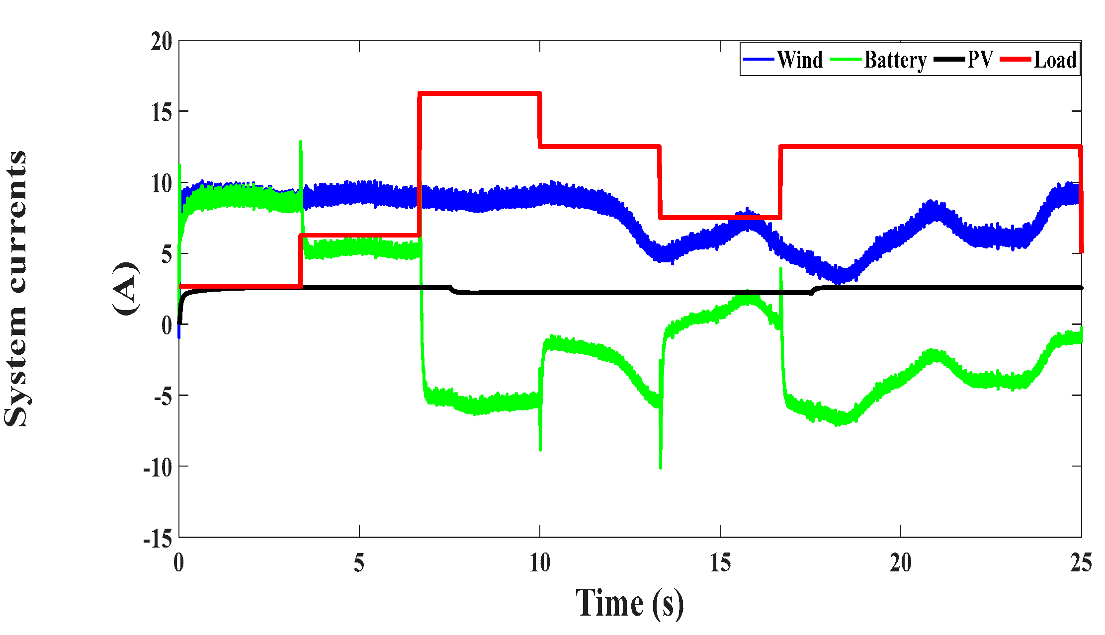
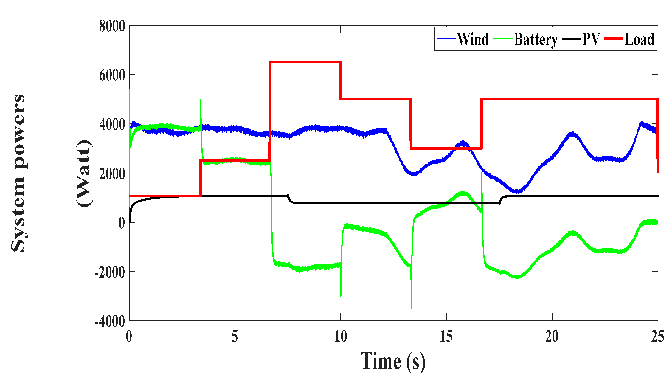
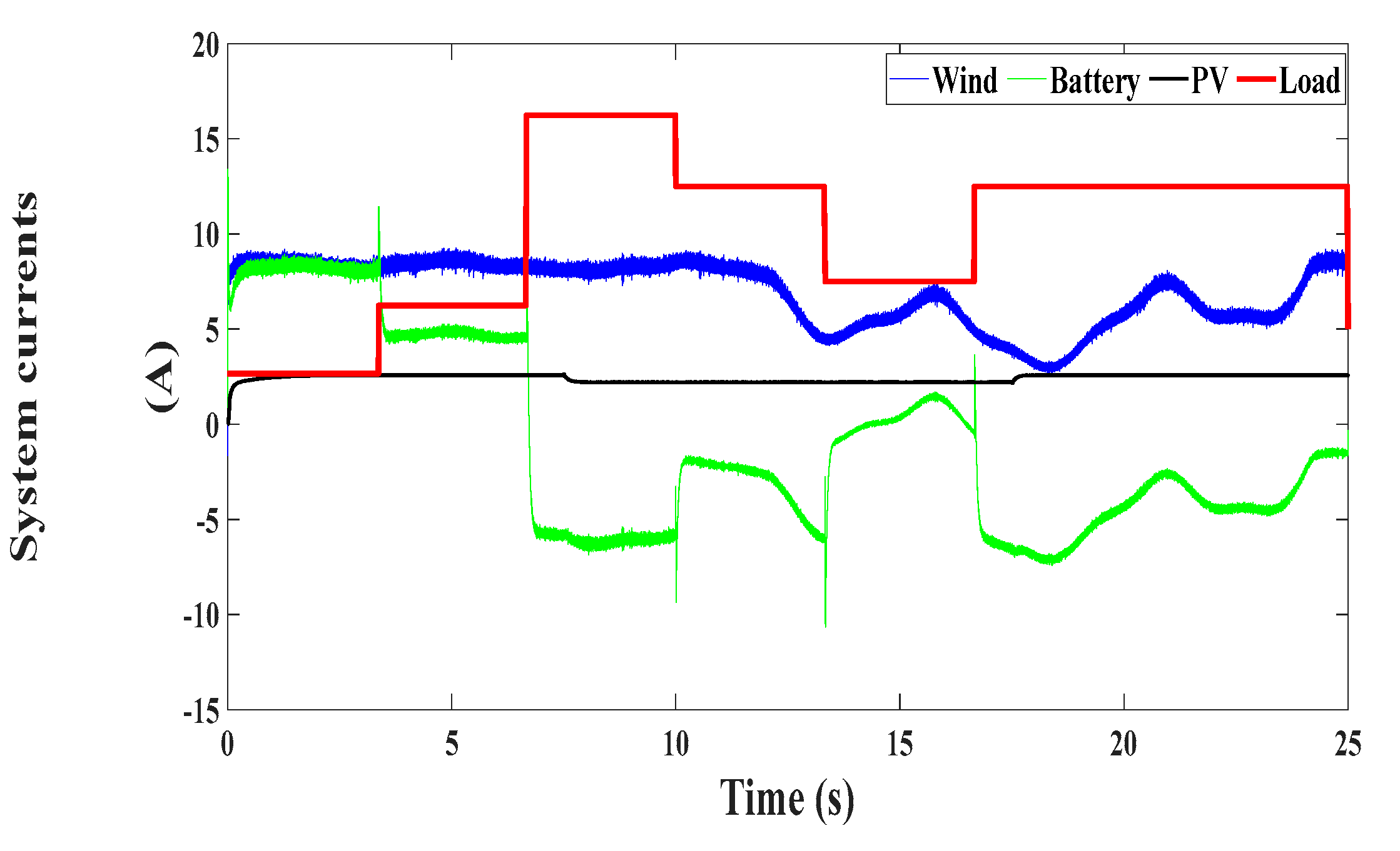
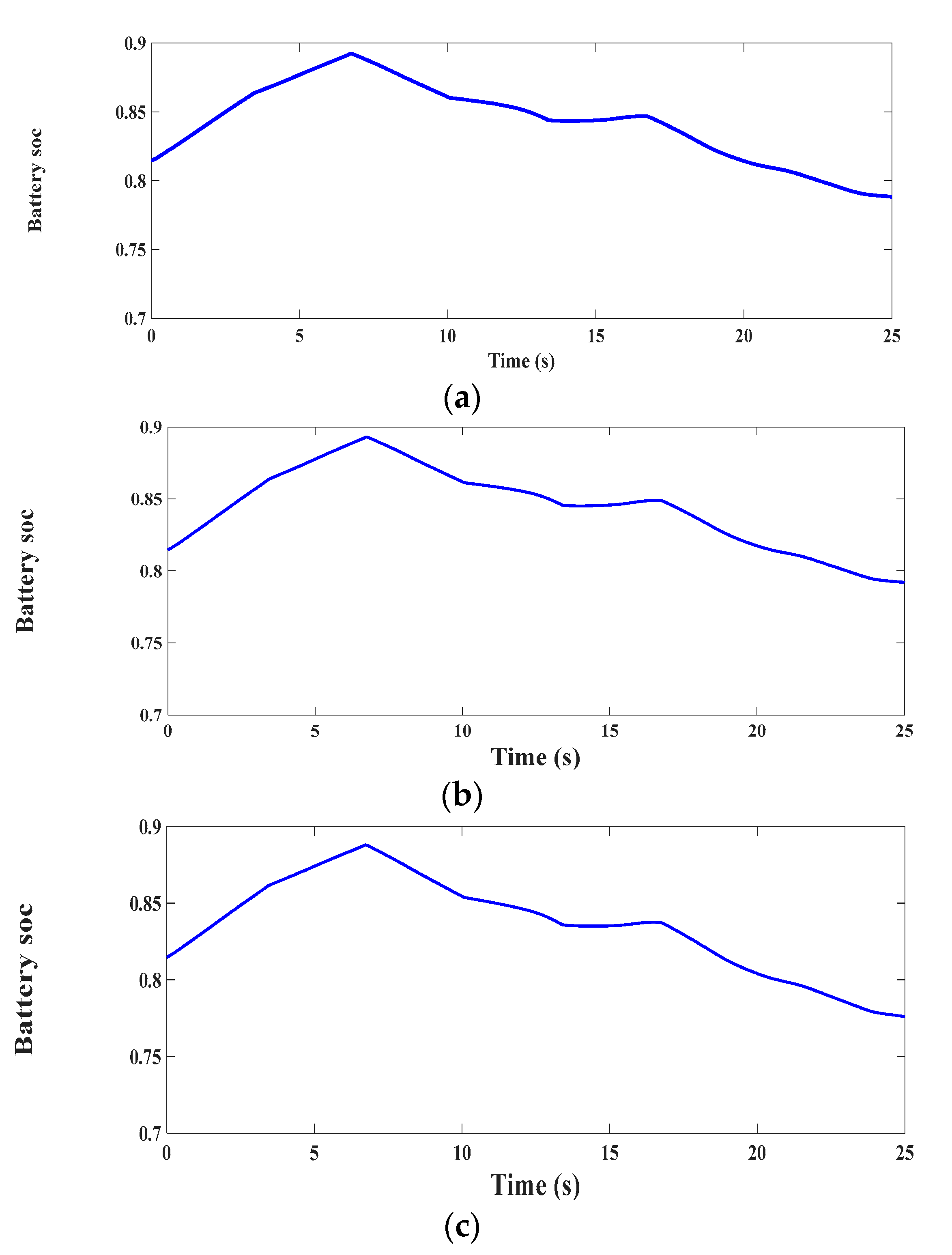
4. Power Management (PM) Topology for Standalone Operation

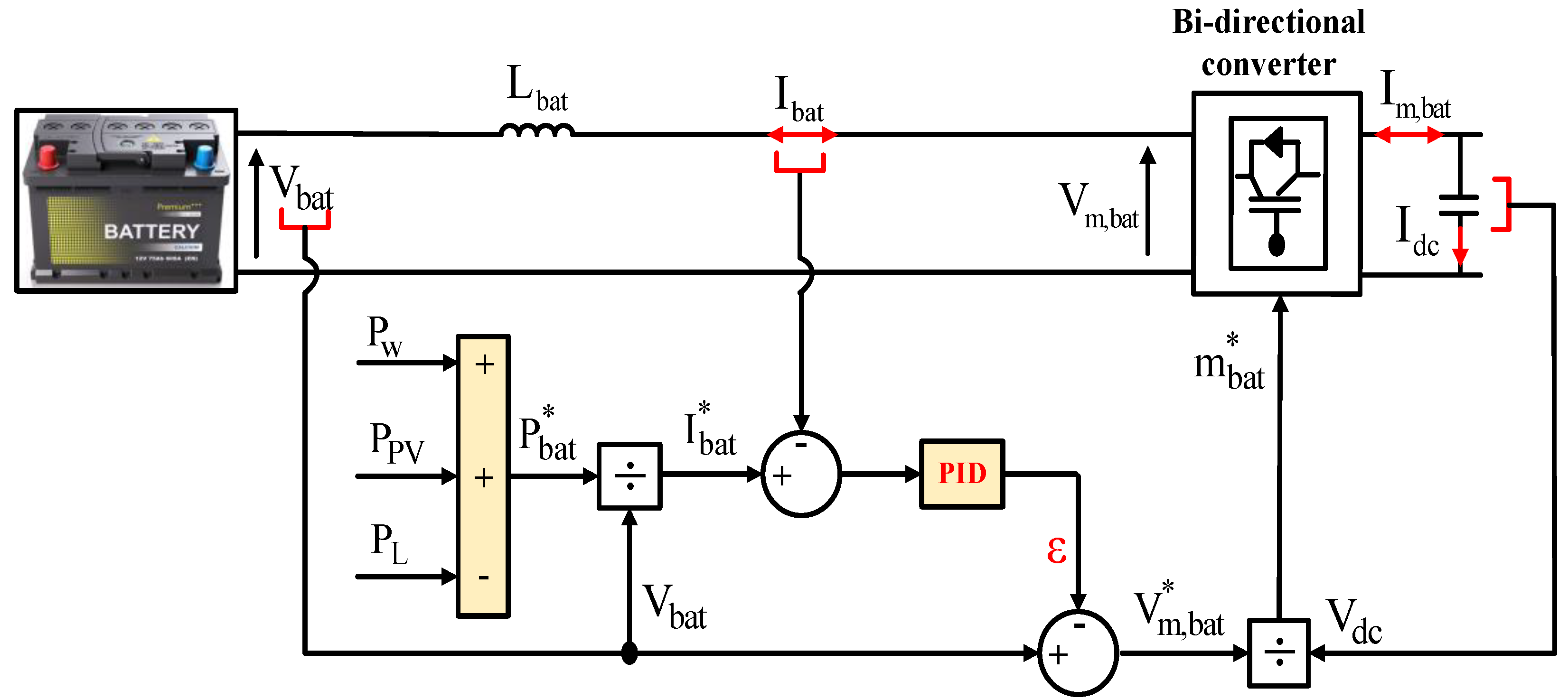
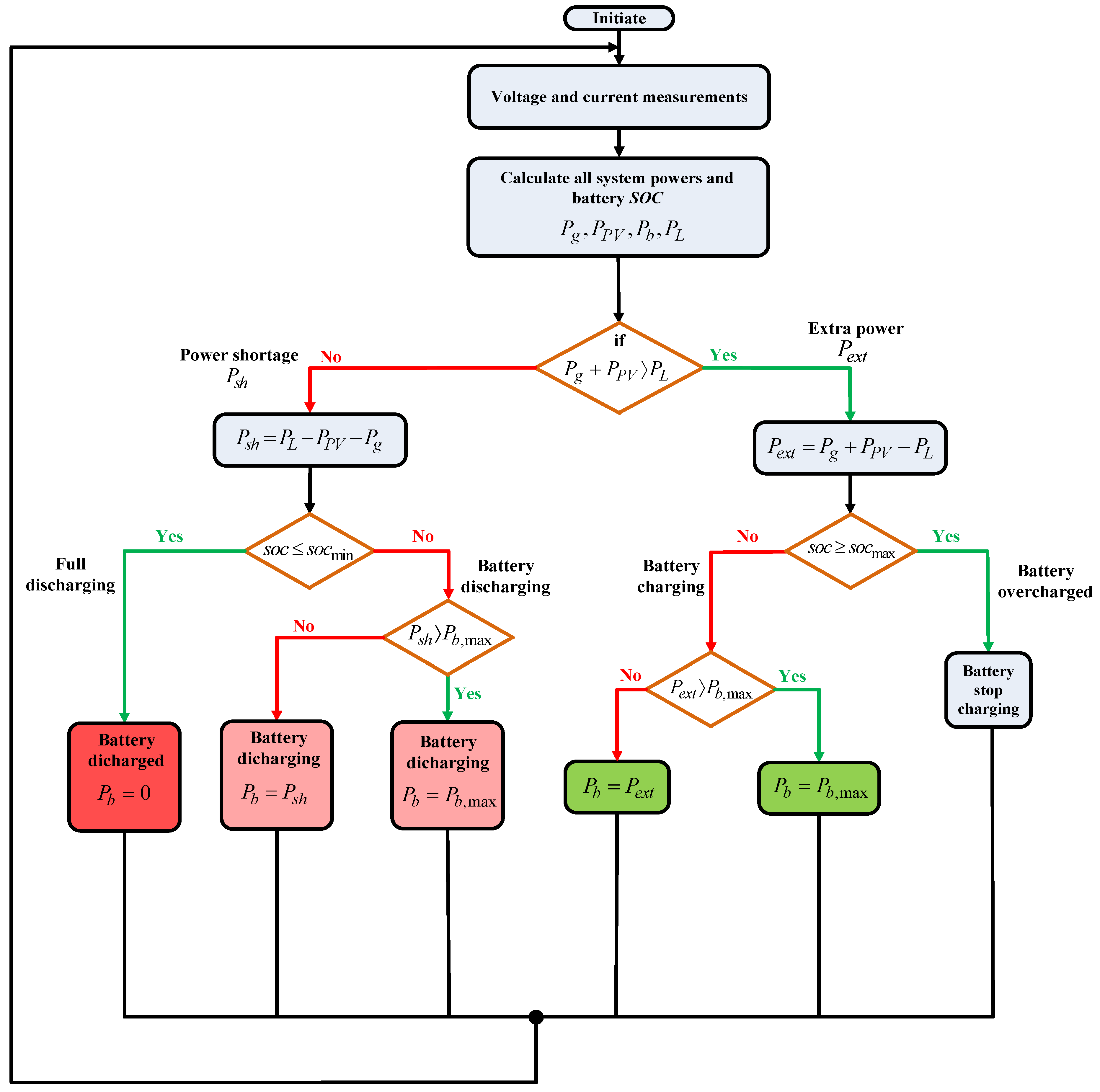
For the standalone operating mode, a particular PM topology is designed to process the solar and wind power systems at full capacity under a variety of environmental situations (i.e., weak wind speed and low irradiation levels). As a result, the PM plan is to balance the power exchange between wind and PV generation systems, battery storage systems, and loads. The PM also regulates the battery’s state of charge (SOC) to prolong battery life.

According to the power flow through the DC connection bus, the power may have various signs. As a result, the PM’s objective is to divide the electricity among these units fairly. The configured PM topology is viewed in Figure 7, and it is observed that when the extra power ${\mathrm{P}}_{\mathrm{ext}}>{\mathrm{P}}_{\mathrm{b},\max }$ is reached, the extra power ${\mathrm{P}}_{\mathrm{ext}}$ will enter the battery when the net power (${\mathrm{P}}_{\mathrm{g}}+{\mathrm{P}}_{\mathrm{PV}}$) exceeds the load power ${\mathrm{P}}_{\mathrm{L}}$ and the condition ${\mathrm{P}}_{\mathrm{ext}}\le {\mathrm{P}}_{\mathrm{b},\max }$ is achieved. When the battery is fully charged or ${\mathrm{P}}_{\mathrm{ext}}>{\mathrm{P}}_{\mathrm{b},\max }$, the extra power cannot be stored and should be restricted. If the produced power ${\mathrm{P}}_{\mathrm{g}}+{\mathrm{P}}_{\mathrm{PV}}$ is less than the load, there would be a power shortfall evaluated by ${\mathrm{P}}_{\mathrm{sh}}=\left[{\mathrm{P}}_{\mathrm{L}}-\left({\mathrm{P}}_{\mathrm{g}}+{\mathrm{P}}_{\mathrm{PV}}\right) \right]$. To counteract the shortage of electricity, the battery will discharge. Due to the finite capacitance, this condition can only be present for a limited period. Calculating the capacity should take into account periods when no energy is provided or when the amount of energy produced is reduced.

5. Evaluation Results

5.1. Results under Grid Connection Mode

The performance evaluation is performed for the grid connection case, in which only the wind generation system is connected to the grid. In this evaluation procedure, the turbine system dynamics are investigated, considering the MPPT and PAC controls. Moreover, the five-phase PMSG dynamics are evaluated using the three predictive schemes (traditional PTC, PFC, and a newly designed predictive scheme). Additionally, the PCC control is used to manage the operation of the GSC converter to ensure unity pf operation. Figure 8 provides the wind speed change ${\mathsf{\omega }}_{\mathrm{w}}$; while Figure 9 illustrates the shaft speed ${\mathsf{\omega }}_{\mathrm{g}}$. From Figure 9, it is confirmed that the shaft speed tracks the wind speed change properly. Figure 10 shows the turbine coefficient ${\mathrm{C}}_{\mathrm{p}}$ from which it is observed that its value changes at each instant that the wind speed overlaps its nominal values, which validates the adopted MPPT and pitch angle controls. This fact is also approved in Figure 11 and Figure 12, which respectively illustrate that the tip ratio $\mathsf{\gamma }$ is preserved at its optimum value (to ensure MPPT), while the balde angle β exhibits an increase each time the wind overlaps the nominal value. All system’s parameters are given in Appendix A.

After that, the five-phase PMSG dynamics are analyzed using the three predictive controllers to visualize the performance of each controller. In Figure 13, the generated powers are shown, from which it is confirmed that the new predictive controller provides reduced power oscillation compared to the classic PTC and PFC schemes, which enhances the quality of the delivered power. This is also ensured by the torque profile in Figure 14. The fact is confirmed in Figure 15, which provides the actual and reference values of generator currents d-q components. The currents are exhibiting reduced ripples using the designed controller compared with the other two predictive schemes. Moreover, it is noticed that the q- axis current emulates the change in the active power and torque profiles. Figure 16 illustrates the DC link voltage dynamics under the three controllers, from which it is clear that the designed control provides much less voltage fluctuation around its reference value. Figure 17 illustrates the grid power signals, from which it is approved that a unity pf operation is properly achieved, while the obtained values have lower ripples under the designed predictive controller. Figure 18, Figure 19 and Figure 20 present the generated five-phase currents under the three controllers. The generated currents are uniformly distributed sinusoidal currents with much fewer harmonics using the designed controller. The current THD analysis under the three controllers is recorded in

Table 1. THD analysis for the grid connection case.

Phase	Classic PTC [34]		PFC [48]		Designed Predictive Controller
	Fundamental	THD	Fundamental	THD	Fundamental	THD
‘a’	11.0326 A	2.85%	9.85307	2.27%	9.7225 A	2.03%
‘b’	10.2785 A	1.76%	9.87774 A	1.74%	9.64383 A	1.68%
‘c’	10.7394 A	2.4%	9.92996 A	2.15%	9.69451 A	1.89%
‘d’	10.7578 A	2.28%	9.76459 A	2.22%	9.69128 A	1.92%
‘e’	10.2665 A	1.86%	9.7734 A	1.81%	9.64583 A	1.67%

, which emphasizes the capability of newly designed controllers in comparison with classic controllers. Additionally, a comparison in terms of the number of computations is addressed in

Table 2. Number of commutations under three controllers.

Classic PTC [34]	PFC [48]	Designed Predictive Controller
1.45 × 104	1.35 × 104	1.04 × 104

, which confirms the superiority of the designed controller in reducing the computation time.

5.2. Results under Standalone Operation

In this test, the wind generation system is hybridized with a PV solar system and a battery to feed a separate load. The effectiveness of the controllers for the five-phase PMSG, DC boost converter, and bi-directional converter is investigated in detail. Additionally, the validity of power flow regulation is investigated. A wind speed variation similar to that adopted in the grid connection mode is adopted and illustrated in Figure 21. The generator’s performance are shown through Figure 22, Figure 23, Figure 24, Figure 25, Figure 26 and Figure 27, which illustrate respectively the generator active and reactive powers, the generator torque, the current components, and the generated five-phase currents using the three predictive controllers. From these illustrations, it is easy to distinguish the effectiveness of the new control in comparison with the traditional PTC and PFC schemes by achieving fewer power and torque fluctuations and fewer current harmonics as well. The PFC, of course, presents better performance than the PTC; however, it is still unable to beat the newly designed PVC. The DC link voltage is also presented in Figure 28. To analyze the current harmonics deeply, the THD analysis for the five-phase currents is presented numerically in

Table 3. THD analysis for standalone operation.

Phase	Classic PTC		PFC		Designed Predictive Controller
	Fundamental	THD	Fundamental	THD	Fundamental	THD
‘a’	10.4947 A	2.43%	10.6124 A	2.16%	9.6333 A	1.11%
‘b’	10.1032 A	1.69%	10.4282 A	1.31%	9.6534 A	1.02%
‘c’	10.2737 A	2.53%	10.5652 A	1.86%	9.5876 A	1.48%
‘d’	10.3919 A	1.96%	10.5726 A	1.25%	9.6739 A	0.74%
‘e’	10.0283 A	2.13%	10.4509 A	1.86%	9.6001 A	1.43%

. By analyzing the THD values, it is approved that the suggested PVC control succeeded in achieving lower current harmonics than the other two controllers. The validity of the designed controller for the PV converter is illustrated through Figure 29, Figure 30, Figure 31 and Figure 32, which show the solar irradiation, the delivered power from the converter, the delivered current, and the output voltage. The control system succeeded in maintaining smooth power tracking for the solar irradiation while maintaining MPPT operation. Additionally, the output voltage is kept properly at its reference value.

The validity of the power regulator and the battery charging/discharging system has been investigated in Figure 33, Figure 34, Figure 35, Figure 36, Figure 37 and Figure 38, which illustrate the power and current exchanges in the system considering the three predictive controllers with the five-phase PMSG. From these illustrations, the validity of the PM system is confirmed in achieving a balanced power flow in the system and preserving smooth charging/discharging processes for the battery. The illustrated power flow can be divided into intervals to give a detailed view of the transfer process, as shown in

Table 4. Power exchange in a hybrid system.

Period	$\left(0\to \frac{20}{6}\right) \mathbf{s}$	$\left(\frac{20}{6}\to \frac{40}{6}\right) \mathbf{s}$	$\left(\frac{40}{6}\to \frac{60}{6}\right) \mathbf{s}$	$\left(\frac{60}{6}\to \frac{80}{6}\right) \mathbf{s}$	$\left(\frac{80}{6}\to \frac{100}{6}\right) \mathbf{s}$	$\left(\frac{100}{6}\to 25\right) \mathbf{s}$
Power state	The load is almost covered from PV power and the battery is charging with a power almost equal to the wind power	The load is increased, and the battery is still charging but with a lower value than that in previous period. The load is covered from both the wind and PV powers.	The load is further increased, and the wind and solar powers together are not sufficient to cover it. Thus, the battery started to discharge to cover the power shortage.	The load Is slightly reduced in this period; however the generated powers are still not totally sufficient. Thus the battery continues to discharge but with a smaller rate than previous interval.	The load continues to decrease, and the combined wind and solar powers are now sufficient to cover the load. The battery as a result starts to recharge again.	The load has an increase again, and there is a shortage in the delivered power which is compensated through discharging the battery.

.

Finally, the charging/discharging processes can be investigated through the battery state charge profiles shown in Figure 39.

6. Conclusions

The presented study aims to enhance the dynamics of a renewable energy system that operates in two different modes: grid connection and standalone. A detailed description of all system units is provided. The system used for grid connection is constructed of a wind-driven five-phase PMSG connected to the grid via a rectifier/DC link/inverter configuration. Alternatively, the system used for standalone operation consisted of a combination of a wind energy system, a PV solar system, a storage battery, and an isolated load. A MPPT tracking strategy is utilized with the wind turbine to maximize its power. The dynamics of the five-phase generator are also enhanced using a newly designed predictive controller. A systematic design for the control of PV converter systems is provided using a combination of the incremental conductance algorithm and a designed regulator. The battery’s operation is regulated using an effective control system. An effective PM procedure is adopted to ensure a balanced power distribution among all units for standalone operation purposes. The evaluation results reveal and affirm the superiority of the proposed scheme in comparison with the classic predictive control. This has been approved by ensuring lower fluctuation in the controlled variables and fewer harmonics in the generated currents, which enhances the quality of the generated power. The results also confirm the validity of the adopted PM procedure under standalone operation. For future works, the designed predictive scheme can be applied for managing the operation of different categories of generators after adopting the operation theory of each topology. Additionally, artificial intelligence-based power management can be considered for balancing the power flow.

References

1. Al Hadi, A.; Silva, C.A.S.; Hossain, E.; Challoo, R. Algorithm for Demand Response to Maximize the Penetration of Renewable Energy. IEEE Access 2020, 8, 55279–55288. [Google Scholar] [CrossRef]
2. Nehrir, M.H.; Wang, C.; Strunz, K.; Aki, H.; Ramakumar, R.; Bing, J.; Miao, Z.; Salameh, Z. A Review of Hybrid Renewable/Alternative Energy Systems for Electric Power Generation: Configurations, Control, and Applications. IEEE Trans. Sustain. Energy 2011, 2, 392–403. [Google Scholar]
3. Hashimoto, J.; Ustun, T.S.; Suzuki, M.; Sugahara, S.; Hasegawa, M.; Otani, K. Advanced Grid Integration Test Platform for Increased Distributed Renewable Energy Penetration in Smart Grids. IEEE Access 2021, 9, 34040–34053. [Google Scholar] [CrossRef]
4. Nurunnabi, M.; Roy, N.K.; Hossain, E.; Pota, H.R. Size Optimization and Sensitivity Analysis of Hybrid Wind/PV Micro-Grids- A Case Study for Bangladesh. IEEE Access 2019, 7, 150120–150140. [Google Scholar] [CrossRef]
5. Sangwongwanich, A.; Yang, Y.; Blaabjerg, F. Development of flexible active power control strategies for grid-connected photovoltaic inverters by modifying MPPT algorithm. In Proceedings of the IEEE 3rd International Future Energy Electronics Conference and ECCE Asia, Kaohsiung, Taiwan, 3–7 June 2017; pp. 87–92. [Google Scholar]
6. Mohandes, B.; Wahbah, M.; Moursi, M.S.E.; El-Fouly, T.H.M. Renewable Energy Management System: Optimum Design and Hourly Dispatch. IEEE Trans. Sustain. Energy 2021, 12, 1615–1628. [Google Scholar]
7. Elmouatamid, A.; Bakhouya, M.; Ouladsine, R.; El kamoun, N.; Zine-Dine, K.; Khaidar, M.; Abid, R. Deployment and Experimental Evaluation of Micro-Grid Systems. In Proceedings of the 2018 6th International Renewable and Sustainable Energy Conference (IRSEC), Rabat, Morocco, 5–8 December 2018; pp. 1–6. [Google Scholar]
8. Mi, Y.; Song, Y.; Fu, Y.; Su, X.; Wang, C.; Wang, J. Frequency and Voltage Coordinated Control for Isolated Wind–Diesel Power System Based on Adaptive Sliding Mode and Disturbance Observer. IEEE Trans. Sustain. Energy 2018, 10, 2075–2083. [Google Scholar] [CrossRef]
9. Jing, W.; Lai, C.H.; Wallace, S.H.; Wong, M.L. Battery-supercapacitor hybrid energy storage system in standalone DC microgrids: A review. IET Renew. Power Gener. 2017, 11, 461–469. [Google Scholar]
10. Xu, X.; Mitra, J.; Wang, T.; Mu, L. Evaluation of Operational Reliability of a Microgrid Using a Short-Term Outage Model. IEEE Trans. Power Syst. 2014, 29, 2238–2247. [Google Scholar] [CrossRef]
11. Pradhan, S.; Murshid, S.; Singh, B.; Panigrahi, B.K. Performance Investigation of Multifunctional On-Grid Hybrid Wind–PV System With OASC and MAF-Based Control. IEEE Trans. Power Electron. 2019, 34, 10808–10822. [Google Scholar] [CrossRef]
12. Wu, Q.; Sun, Y.; Navid, Z.; Samir, K. Modeling and Modern Control of Wind Power; John Wiley & Sons: New York, NY, USA, 2018. [Google Scholar]
13. Kong, X.; Liu, X.; Ma, L.; Lee, K.Y. Hierarchical Distributed Model Predictive Control of Standalone Wind/Solar/Battery Power System. IEEE Trans. Syst. Man Cybern. Syst. 2019, 49, 1570–1581. [Google Scholar] [CrossRef]
14. Zhu, Y.; Zhao, R.; Zhao, J. Output power smoothing control for the PMSG based wind farm by using the allocation of the wind turbines. In Proceedings of the 20th International Conference on Electrical Machines and Systems (ICEMS), Sydney, NSW, Australia, 11–14 August 2017; pp. 1–6. [Google Scholar]
15. Gajewski, P.; Pieńkowski, K. Control of wind turbine system with PMSG for low voltage ride through. In Proceedings of the International Symposium on Electrical Machines, Andrychow, Poland, 10–13 June 2018; pp. 1–6. [Google Scholar]
16. Gul, W.; Gao, Q.; Lenwari, W. Optimal Design of a 5-MW Double-Stator Single-Rotor PMSG for Offshore Direct Drive Wind Turbines. IEEE Trans. Ind. Appl. 2019, 56, 216–225. [Google Scholar] [CrossRef]
17. Delavaripour, H.; Dehkordi, B.M.; Zarchi, H.A.; Adib, E. Increasing Energy Capture From Partially Shaded PV String Using Differential Power Processing. IEEE Trans. Ind. Electron. 2018, 66, 7672–7682. [Google Scholar] [CrossRef]
18. de Souza, A.C.; Melo, F.C.; Oliveira, T.L.; Tavares, C.E. Performance Analysis of the Computational Implementation of a Simplified PV Model and MPPT Algorithm. IEEE Lat. Am. Trans. 2016, 14, 792–798. [Google Scholar] [CrossRef]
19. Pragallapati, N.; Agarwal, V. Distributed PV Power Extraction Based on a Modified Interleaved SEPIC for Nonuniform Irradiation Conditions. IEEE J. Photovolt. 2015, 5, 1442–1453. [Google Scholar] [CrossRef]
20. Vanco, W.E.; Silva, F.B.; Goncalves, F.A.S.; Bissochi, C.A. Evaluation of the Capacitor Bank Design for Self-Excitation in Induction Generators. IEEE Lat. Am. Trans. 2018, 16, 482–488. [Google Scholar] [CrossRef]
21. Teng, K.; Lu, Z.; Long, J.; Wang, Y.; Roskilly, A.P. Voltage Build-Up Analysis of Self-Excited Induction Generator With Multi-Timescale Reduced-Order Model. IEEE Access 2019, 7, 48003–48012. [Google Scholar] [CrossRef]
22. Prince, M.K.K.; Arif, M.T.; Gargoom, A.; Oo, A.M.T.; Haque, M.E. Modeling, Parameter Measurement, and Control of PMSG based Grid-connected Wind Energy Conversion System. J. Mod. Power Syst. Clean Energy 2021, 9, 1054–1065. [Google Scholar]
23. Wang, X.; Sala, G.; Zhang, H.; Gu, C.; Buticchi, G.; Formentini, A.; Gerada, C.; Wheeler, P. Torque Ripple Reduction in Sectored Multi Three-Phase Machines Based on PWM Carrier Phase Shift. IEEE Trans. Ind. Electron. 2019, 67, 4315–4325. [Google Scholar] [CrossRef]
24. Rubino, S.; Bojoi, R.; Cittanti, D.; Zarri, L. Decoupled and Modular Torque Control of Multi-Three-Phase Induction Motor Drives. IEEE Trans. Ind. Appl. 2020, 56, 3831–3845. [Google Scholar] [CrossRef]
25. Mossa, M.A.; Quynh, N.V.; Echeikh, H.; Do, T.D. Deadbeat-Based Model Predictive Voltage Control for a Sensorless Five-Phase Induction Motor Drive. Math. Probl. Eng. 2020, 2020, 4164526. [Google Scholar] [CrossRef]
26. Li, G.; Hu, J.; Li, Y.; Zhu, J. An Improved Model Predictive Direct Torque Control Strategy for Reducing Harmonic Currents and Torque Ripples of Five-Phase Permanent Magnet Synchronous Motors. IEEE Trans. Ind. Electron. 2018, 66, 5820–5829. [Google Scholar] [CrossRef]
27. Mossa, M.A.; Echeikh, H.; Diab, A.A.Z.; HaesAlhelou, H.; Siano, P. Comparative Study of Hysteresis Controller, Resonant Controller and Direct Torque Control of Five-Phase IM under Open-Phase Fault Operation. Energies 2021, 14, 1317. [Google Scholar] [CrossRef]
28. Wu, S.; Tian, C.; Zhao, W.; Zhou, J.; Zhang, X. Design and Analysis of an Integrated Modular Motor Drive for More Electric Aircraft. IEEE Trans. Transp. Electrif. 2020, 6, 1412–1420. [Google Scholar] [CrossRef]
29. Rhaili, S.; Abbou, A.; Marhraoui, S.; El Hichami, N.; Hemeyine, A.V. Robustness investigation of Vector Control of Five-phase PMSG based Variable-Speed Wind Turbine under faulty condition. In Proceedings of the 2018 Renewable Energies, Power Systems & Green Inclusive Economy (REPS-GIE), Casablanca, Morocco, 23–24 April 2018; pp. 1–6. [Google Scholar]
30. Dieng, A.; Le Claire, J.C.; Mboup, A.B.; Benkhoris, M.F.; Ait-Ahmed, M. An improved torque control strategy of “five-phase PMSG-PWM rectifier” set for marine current turbine applications. In Proceedings of the 2019 IEEE 13th International Conference on Compatibility, Power Electronics and Power Engineering (CPE-POWERENG), Sonderborg, Denmark, 23–25 April 2019; pp. 1–6. [Google Scholar]
31. Mekri, F.; Ben Elghali, S.; Benbouzid, M.E.H. Fault-Tolerant Control Performance Comparison of Three- and Five-Phase PMSG for Marine Current Turbine Applications. IEEE Trans. Sustain. Energy 2012, 4, 425–433. [Google Scholar] [CrossRef] [Green Version]
32. Hoerner, M.; Wendel, S.; Dietz, A.; Karamanakos, P.; Kennel, R. Variable Switching Point Predictive Current Control for Multi-Phase Permanent Magnet Synchronous Drives. In Proceedings of the 2021 IEEE International Conference on Predictive Control of Electrical Drives and Power Electronics (PRECEDE), Jinan, China, 20–22 November 2021; pp. 184–189. [Google Scholar]
33. Yip, S.Y.; Yong, D.W.; Yiauw, K.H.; Tan, X.J.; Wong, J.Y.R. Model Predictive Direct Torque with Fault Tolerance Control for a Permanent Magnet Synchronous Generator Based on Vienna Rectifier. IEEE Access 2022, 10, 94998–95007. [Google Scholar] [CrossRef]
34. Jlassi, I.; Cardoso, A.J.M. Open-circuit fault-tolerant operation of permanent magnet synchronous generator drives for wind turbine systems using a computationally efficient model predictive current control. IET Electr. Power Appl. 2021, 15, 837–846. [Google Scholar] [CrossRef]
35. Alizadeh, O.; Yazdani, A. A Strategy for Real Power Control in a Direct-Drive PMSG-Based Wind Energy Conversion System. IEEE Trans. Power Deliv. 2013, 28, 1297–1305. [Google Scholar] [CrossRef]
36. Yip, S.Y.; Che, H.S.; Tan, C.P.; Chong, W.T. A Lookup Table Model Predictive Direct Torque Control of Permanent-Magnet Synchronous Generator Based on Vienna Rectifier. IEEE J. Emerg. Sel. Top. Power Electron. 2019, 8, 1208–1222. [Google Scholar] [CrossRef]
37. Mossa, M.A. Effective predictive current control for a sensorless five-phase induction motor drive. Int. J. Power Electron. 2021, 13, 502. [Google Scholar] [CrossRef]
38. Kamel, T.; Abdelkader, D.; Said, B.; Padmanaban, S.; Iqbal, A. Extended Kalman Filter Based Sliding Mode Control of Parallel-Connected Two Five-Phase PMSM Drive System. Electronics 2018, 7, 14. [Google Scholar] [CrossRef] [Green Version]
39. Hazari, R.; Jahan, E.; Mannan, M.A.; Das, N. Transient Stability Enhancement of a Grid-Connected Large-Scale PV System Using Fuzzy Logic Controller. Electronics 2021, 10, 2437. [Google Scholar] [CrossRef]
40. Memon, A.; Mustafa, M.W.; Aman, M.N.; Hafeez, A.; Ullah, M. Improving Transient Behavior of a Brushless Doubly Fed Induction Generator through Reactive Current Control of Grid-Side Converter. Electronics 2021, 10, 1413. [Google Scholar] [CrossRef]
41. Venkatesan, K.; Govindarajan, U. Optimal power flow control of hybrid renewable energy system with energy storage: A WOANN strategy. J. Renew. Sustain. Energy 2019, 11, 015501. [Google Scholar] [CrossRef]
42. Kucuker, A.; Kamal, T.; Hassan, S.Z.; Li, H.; Mufti, G.M.; Waseem, M. Design and control of photovoltaic/wind/battery based microgrid system. In Proceedings of the 2017 International Conference on Electrical Engineering (ICEE), Lahore, Pakistan, 2–4 March 2017; pp. 1–6. [Google Scholar] [CrossRef]
43. Bhangu, B.; Bentley, P.; Stone, D.; Bingham, C. Nonlinear Observers for Predicting State-of-Charge and State-of-Health of Lead-Acid Batteries for Hybrid-Electric Vehicles. IEEE Trans. Veh. Technol. 2005, 54, 783–794. [Google Scholar] [CrossRef] [Green Version]
44. Owusu-Nyarko, I.; Elgenedy, M.A.; Abdelsalam, I.; Ahmed, K.H. Modified Variable Step-Size Incremental Conductance MPPT Technique for Photovoltaic Systems. Electronics 2021, 10, 2331. [Google Scholar] [CrossRef]
45. Chankaya, M.; Hussain, I.; Malik, H.; Ahmad, A.; Alotaibi, M.A.; Márquez, F.P.G. Seamless Capable PV Power Generation System without Battery Storage for Rural Residential Load. Electronics 2022, 11, 2413. [Google Scholar] [CrossRef]
46. Mossa, M.A.; Gam, O.; Bianchi, N.; Quynh, N.V. Enhanced Control and Power Management for a Renewable Energy-Based Water Pumping System. IEEE Access 2022, 10, 36028–36056. [Google Scholar] [CrossRef]
47. Saavedra, J.L.; Baier, C.R.; Marciel, E.I.; Rivera, M.; Carreno, A.; Hernandez, J.C.; Melín, P.E. Comparison of FCS-MPC Strategies in a Grid-Connected Single-Phase Quasi-Z Source Inverter. Electronics 2023, 12, 2052. [Google Scholar] [CrossRef]
48. Fu, R. Robust Model Predictive Flux Control of PMSM Drive Using a Compensated Stator Flux Predictor. IEEE Access 2021, 9, 136736–136743. [Google Scholar] [CrossRef]
Figure 1. System under study: (a) grid connection case; (b) standalone operation.
Electronics 12 03408 g001
Figure 2. (a) Solar cell. (b) Solar array.
Electronics 12 03408 g002
Figure 3. Battery equivalent circuit.
Electronics 12 03408 g003
Figure 4. Control scheme of the battery bi-directional converter.
Electronics 12 03408 g004
Figure 5. MPPT system based on a combined ICA and PID controller.
Electronics 12 03408 g005
Figure 6. Schematic diagram of the newly designed predictive controller for five-phase PMSG.
Electronics 12 03408 g006
Figure 7. Power management topology for standalone operation.
Electronics 12 03408 g007
Figure 8. Wind speed profile.
Electronics 12 03408 g008
Figure 9. Generator speed.
Electronics 12 03408 g009
Figure 10. Turbine power coefficient.
Electronics 12 03408 g010
Figure 11. Tip ratio.
Electronics 12 03408 g011
Figure 12. Blade angle.
Electronics 12 03408 g012
Figure 13. Generated powers.
Electronics 12 03408 g013
Figure 14. Generator torque.
Electronics 12 03408 g014
Figure 15. Generator current d-q components (A).
Electronics 12 03408 g015
Figure 16. DC bus voltage.
Electronics 12 03408 g016
Figure 17. Grid powers.
Electronics 12 03408 g017
Figure 18. Generator currents under classic PTC.
Electronics 12 03408 g018
Figure 19. Generator currents under PFC.
Electronics 12 03408 g019
Figure 20. Generator currents under the proposed controller.
Electronics 12 03408 g020
Figure 21. Wind speed variation.
Electronics 12 03408 g021
Figure 22. Generated power for standalone operation.
Electronics 12 03408 g022
Figure 23. Developed generator torque.
Electronics 12 03408 g023
Figure 24. Generator current components (A).
Electronics 12 03408 g024
Figure 25. Five phase generated currents under PTC (A).
Electronics 12 03408 g025
Figure 26. Five phase generated currents under PFC (A).
Electronics 12 03408 g026
Figure 27. Five phase generated currents under proposed control (A).
Electronics 12 03408 g027
Figure 28. DC bus voltage for standalone operation (V).
Electronics 12 03408 g028
Figure 29. Solar irradiation.
Electronics 12 03408 g029
Figure 30. Delivered power from the PV system.
Electronics 12 03408 g030
Figure 31. Delivered current from the PV system.
Electronics 12 03408 g031
Figure 32. PV converter output voltage.
Electronics 12 03408 g032
Figure 33. System powers flow considering the PTC controller.
Electronics 12 03408 g033
Figure 34. System currents flow considering the PTC controller.
Electronics 12 03408 g034
Figure 35. System powers flow considering the PFC controller.
Electronics 12 03408 g035
Figure 36. System current flow considering the PFC controller.
Electronics 12 03408 g036
Figure 37. System powers flow considering the proposed controller.
Electronics 12 03408 g037
Figure 38. System currents flow considering the proposed controller.
Electronics 12 03408 g038
Figure 39. Battery SOC: (a) PTC, (b) PFC, and (c) Proposed.
Electronics 12 03408 g039