Low Cost PID Controller for Student Digital Control Laboratory Based on Arduino or STM32 Modules

Abstract

In the teaching process, it is important that students do not carry out exercises only by computer simulations, but also that they carry out research in real time. In times of distance learning during the COVID-19 pandemic, it would be necessary to find a solution so that the students can perform such exercises individually at home. Therefore, it has become necessary to develop cheap and simple modules of digital controllers along with analog objects with adjustable order and time constants. This paper describes a low-cost proportional–integral–derivative (PID) controller for teaching students control techniques and analog control objects in real time. The PID controller is based on the cheap and widely available microcontroller modules Arduino or STM32. The advantage of this solution is that the algorithm of the digital PID controller is calculated every constant period of time. Both the solutions presented in the paper have been successfully tested by students in practice during remote learning during the COVID-19 pandemic.

1. Introduction

The student digital control laboratory aims to teach the student how to design and implement automatic control systems. These systems have many practical uses, such as in cars, planes, robots, factories, processes, space structures, and more. The student starts by learning the basic software and hardware for control systems and the technologies for sensors and actuators. Then, the student creates a control system, tests it in one of the laboratory platforms, and checks whether it meets the design requirements.

Typically in the student digital control laboratory, programs such as Matlab, Matlab-Simulink, Octave, LabView, Psim, Pspice, etc., are used for simulation tests. Performing such simulation tests is a very good complement to the theoretical knowledge gained during lectures. In the course of further research, it is necessary to supplement the knowledge related to the implementation of digital control algorithms in real control systems.

My many years of teaching practice show that during the process of teaching about automatic control systems, the contact of students with a live automatic control system is also important. Such contact works better on the imagination of students and allows a better understanding of the theoretical dependencies specific to automatic control systems.

For this purpose, ready-made modules specially designed for this type of laboratory are used. For example, these can be modules from National Instruments NI myRIO [1] or Speedgoat systems [2]. Unfortunately, such systems are quite expensive and it is difficult to persuade students to use them in the case of distance learning, as was the case during the COVID-19 pandemic.

A cheaper solution is to use modules with microcontrollers and implement digital control algorithms using C/C++. For this purpose, a module with a microcontroller could be used, such as AVR, ARM, TMS320F28xxx, PIC, ADUC84x, etc. [3,4,5,6]. In the case of 8-bit AVR microcontrollers, the most popular is the Arduino platform [7], while for 32-bit ARM micro-controllers, the most popular platforms such as Rasberry Pi, BeagleBone, STM32, and also Arduino can be used [7,8,9,10].

Attention should also be paid to entire families of microcontrollers from Microchip to 8-bit PIC MCUs, 16-bit MCUs, dsPIC33 digital signal controllers and 32-bit MCUs [11]. For student activities, one can also use the Microchip University Program [12]. For rapid prototyping, Microchip has prepared the Curiosity Nano Platform [13]. A good implementation of the PID controller can be found in [14].

Among the cheapest of these are Arduino and STM32, which is why they were chosen. The low prices of microcontroller modules allow the adoption of a solution in which each student has his/her own module with a microcontroller. There is an advantage to using Arduino modules, i.e., the use of a simplified programming environment. This makes it easier to work with students for whom computer science is not their main field of study, for example, students of electrical engineering. However, Arduino software, due to its simplifications, does introduce some limitations.

In the case of modules with STM32 microcontrollers, the manufacturer’s software STM32CubeIDE can be used [10]. The STM32CubeIDE is an advanced C/C++ development platform with peripheral configuration, code generation, code compilation, and debugging capabilities for STM32 microcontrollers and microprocessors. It is based on the Eclipse^®/CDT™ framework, and the GCC toolchain for development and GDB for debugging [10]. The development platform is no longer so simple for students, and requires them to be more involved. It should be noted, however, that the capabilities of ARM microcontrollers are much greater than those of AVR.

The paper focuses on the implementation of the proportional–integral–derivative (PID) controller using Arduino Uno and STM32. On the Arduino website one can find many functions with ready-made programs to implement the PID controller [15,16,17,18,19,20,21,22,23,24,25,26,27,28]. All of these execute the PID algorithm in the main loop of the program, and the sampling period is variable and depends on the complexity of the main program. For the correct determination of the integral and differential, the system time is taken and the time since the last call of the PID algorithm is calculated. This is only acceptable for slowly-varying simple control objects. For more demanding control objects such as power electronics, circuits, quadcopters, etc., this solution cannot be used.

The proposed solution uses a fixed sampling period. Thanks to this, the big value of jitter and the formation of beating output signals can be avoided, which significantly improves the quality of control. In this way, students also learn the correct methods of programming systems working in real time.

Another problem to be solved is the realization of the controlled systems. It was assumed that the time constants of controlled systems would be from one to several seconds, and from one to several orders. For simplicity, it was also assumed that the controlled systems will be powered directly by the microcontroller module. Adopting such a solution is safe because students do not always cope well with systems powered by many sources. In the simplest solution, simple passive RC systems were used as an object. It is also possible to use the active version of the controlled system, using rail-to-rail operational amplifiers, also powered by the microcontroller module. This solution allows for the implementation of a wider range of transmittance compared to passive systems.

During the tests, it is also necessary to measure and record signals; for this purpose, one of the cheap USB oscilloscopes can be used. The Serial Analyzer can be used if an Arduino module is being used [7].

In Section 2, an example of converting the analog PID controller to a digital version is presented. Simple object simulators are described in Section 3. Section 4 is devoted to the implementation of the digital PID controller using the Arduino Uno module. Examples of laboratory test results are also shown. Section 5 is devoted to the implementation of the digital PID controller using the STM32 microcontroller. Also, in this case, sample results of laboratory tests are shown. Section 6 briefly discusses the methods for selecting the parameters of the PID controller.

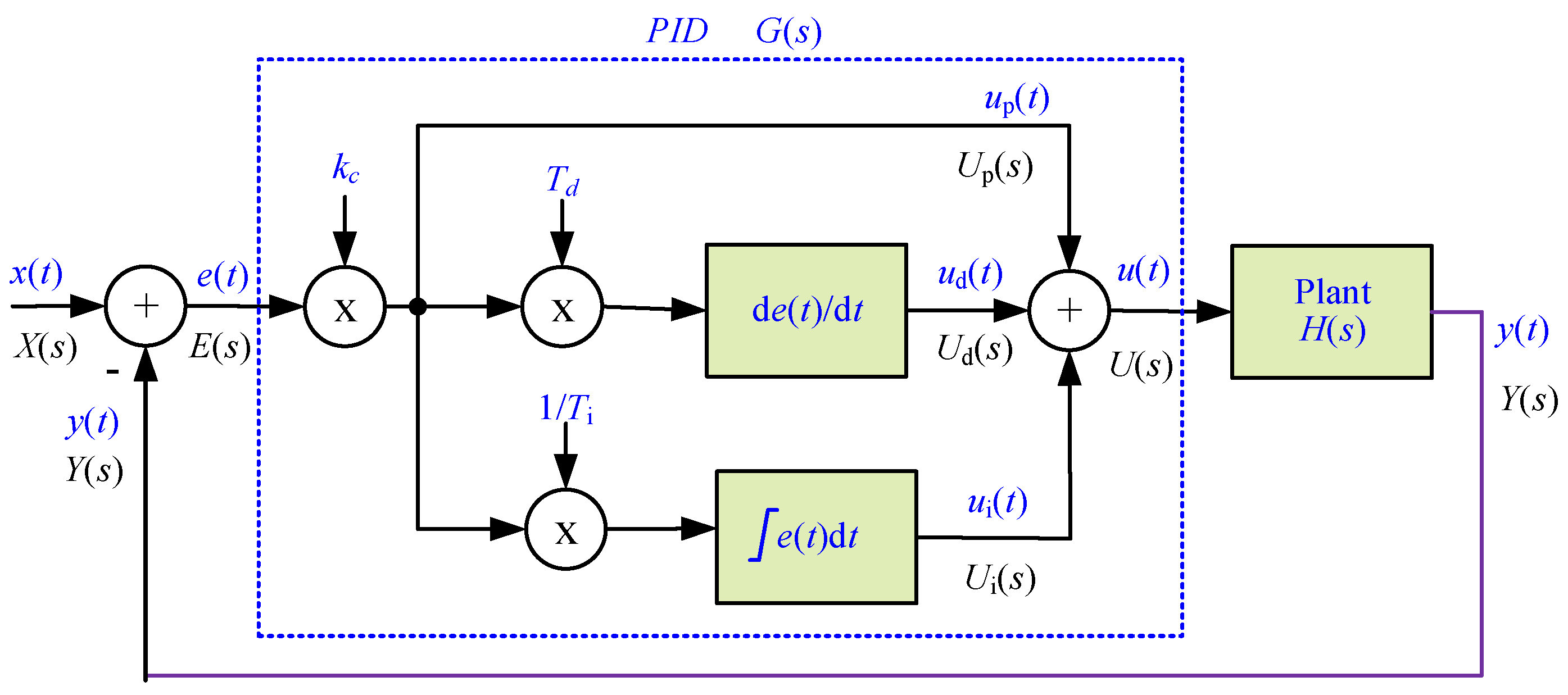
2. Realization of Digital PID Controller

A block diagram of the automatic control system is shown in Figure 1. The system consists of a controller with transfer function G(s) of an object (plant, controlled system, system) with transfer function H(s) and a summation node in which the setpoint X(s) is compared with the output signal Y(s) [29,30,31,32,33,34].

For this control system, a system of equations can be written,

$$\left\{\begin{array}{c}Y\left(s\right)=E\left(s\right)G\left(s\right)H\left(s\right)\\ E\left(s\right)=X\left(s\right)-Y\left(s\right) ,\end{array}\right.$$

(1)

where the following pertains:

• X(s)—desired process value or setpoint;
• E(s)—error value as the difference between a desired setpoint X(s) and the measured process value Y(s), E(s) = X(s) − Y(s);
• G(s)—controller transfer function;
• H(s)—transfer function of controlled system (plant);
• Y(s)—measured process value;
• U(s)—control variable.

From the system of Equation (1) it is possible to determine the transfer function of a closed loop control system

$$\frac{Y\left(s\right)}{X\left(s\right)}=\frac{G\left(s\right)H\left(s\right)}{1+G\left(s\right)H\left(s\right)}$$

(2)

The block diagram of a PID controller is shown in Figure 1. The transfer function of the analog PID controller transmittance of the regulator is determined by the equation

$$G\left(s\right)=\frac{U\left(s\right)}{E\left(s\right)}=k_c\left(1+\frac{1}{T_i}\frac{1}{s}+T_{d}s\right)$$

(3)

where the following pertains:

• k_c—controller gain, a tuning parameter;
• T_d—derivative time, a tuning parameter;
• T_i—integral time, a tuning parameter.

For a PID controller, the control value U(s) consists of three terms: U_p(s)—proportional term, U_i(s)—integral term, U_d(s)—derivative term. The value of the PID controller control variable can be determined using the equation

$$U\left(s\right)=\stackrel{U_p\left(s\right)}{\overbrace{E\left(s\right)k_c}}+\stackrel{U_i\left(s\right)}{\overbrace{\frac{k_c}{T_i}\frac{1}{s}E\left(s\right)}}+\stackrel{U_d\left(s\right)}{\overbrace{k_c{T}_{d}E\left(s\right)s}}$$

(4)

Integral term (4) is transferred into digital form using bilinear transformation

$$s=\frac{T_s}{2}\frac{z+1}{z-1}$$

(5)

where T_s is the sampling period.

$$U_i\left(z\right)=\stackrel{U_i\left(z\right)}{\overbrace{k_c\frac{T_s}{2T_i}\left(E\left(z\right)+E\left(z\right)z^{-1}\right)+U_i\left(z\right)z^{-1}}}$$

(6)

The derivative term is transferred to digital form using backward difference transformation

$$s=\frac{z-1}{T_{s}z}$$

(7)

$$U_d\left(z\right)=\stackrel{U_d\left(z\right)}{\overbrace{k_c\frac{T_d}{T_s}\left(E\left(z\right)-E\left(z\right)z^{-1}\right)}}$$

(8)

Finally, the digital control variable can be determined from the equation

$$U\left(z\right)=\stackrel{U_p\left(z\right)}{\overbrace{E\left(z\right)k_c}}+\stackrel{U_i\left(z\right)}{\overbrace{k_c\frac{T_s}{2T_i}\left(E\left(z\right)+E\left(z\right) z^{-1}\right)+U_i\left(z\right)z^{-1}}}+\stackrel{U_d\left(z\right)}{\overbrace{k_c\frac{T_d}{T_s}\left(E\left(z\right)-E\left(z\right)z^{-1}\right)}}$$

(9)

while the value of the digital control variable can be calculated using the difference equation

$$\begin{array}{cc}u\left(n\right)=\stackrel{u_p\left(n\right)}{\overbrace{k_{c}e\left(n\right)}}+& \stackrel{u_i\left(n\right)}{\overbrace{k_c\frac{T_s}{2T_i}\left(e\left(n\right)+e\left(n-1\right)\right)+u_i\left(n-1\right)}}\hfill \\ & +\stackrel{u_d\left(n\right)}{\overbrace{k_c\frac{T_d}{T_s}\left(e\left(n\right)-e\left(n-1\right)\right)}}\hfill \end{array}$$

(10)

The block diagram of such a digital PID controller is depicted in Figure 2.

It was assumed that in order to simplify the implementation, the PID controller algorithm will be implemented using floating point arithmetic. A range of variability of variables of −1.0…1.0 was also assumed. In addition, saturation of the variables u_i(n) and u(n) has been added to the algorithm.

The digital control variable u(n) is typically converted to an analog form by a D/A converter. Often, as in this case, a PWM modulator is also used as a D/A converter. Before D/A conversion, the control variable u(n) should be scaled to the range of the D/A converter and cast to the integer type

$$u_N\left(n\right)=\left(\mathrm{int}\right)\left(\left(1+u\left(n\right)\right)0.5N_L\right)$$

(11)

where N_L is the number of states of the digital PWM modulator or D/A converter.

The variable range u_N(n) is 0 … N_L − 1. The block diagram of the digital PID controller with saturation, and with a PWM modulator on the output, is shown in Figure 3. This variant of the regulator was adopted for implementation using microcontrollers. Of course, in the literature, it is possible to find many other implementations [29,30,31,32,33,34] of the digital PID controller that can be used here.

For example, by performing a simple modification of the algorithm, one can eliminate the effect of changing the setpoint on the derivative term. The block diagram of such a solution is shown in Figure 4.

It was assumed that the sampling frequency of f_s signals is constant and that the algorithm of the digital PID controller is calculated with the same frequency.

3. Controlled System Simulators

It was assumed that the regulator together with the controlled system must be resistant to assembly errors, easy to implement, and cheap. Therefore, it was assumed that the controlled system should be powered by the microcontroller module. Therefore, the simplest RC systems were used to simulate dynamic objects. Figure 5 shows a two-stage RC network that forms a second-order controlled system. This circuit is limited because its quality factor Q is always less than 0.5, with R₁ = R₂ and C₁ = C₂, Q = 1/3. In this circuit, Q approaches the maximum value of 1/2 when the impedance of the second RC stage is much larger than the first.

The transfer function of the two-stage RC network can also be expressed in

$$H\left(s\right)=\frac{1}{1+s\left(R_1{C}_1+R_2{C}_2+R_1{C}_2\right)+s^2\left(R_1{C}_1{R}_2{C}_2\right)}$$

(12)

Larger values of the quality factor Q are attainable using a positive feedback amplifier. Figure 6 shows an operational amplifier used in this manner. Capacitor C₁, no longer connected to the ground, provides a positive feedback path. These circuits were described in 1955 by R. P. Sallen and E. L. Key, and hence they are generally known as Sallen–Key filters [35,36]. The operational amplifier is a rail-to-rail input–output, and is supplied by a microcontroller module (+5 V for Arduino, and 3.3 V for STM32).

The transfer function of the second-order active object simulator for the position of the switch S₁ in the on position is

$$H\left(s\right)=\frac{\stackrel{k}{\overbrace{\frac{R_3+R_4}{R_3}}}}{1+s\left(R_1{C}_2+R_2{C}_2+R_1{C}_1\left(-\frac{R_4}{R_3}\right)\right)+s^2\left(R_1{C}_1{R}_2{C}_2\right)}$$

(13)

where k—is the plant gain.

Using the circuits shown above, it is possible to build higher-order systems.

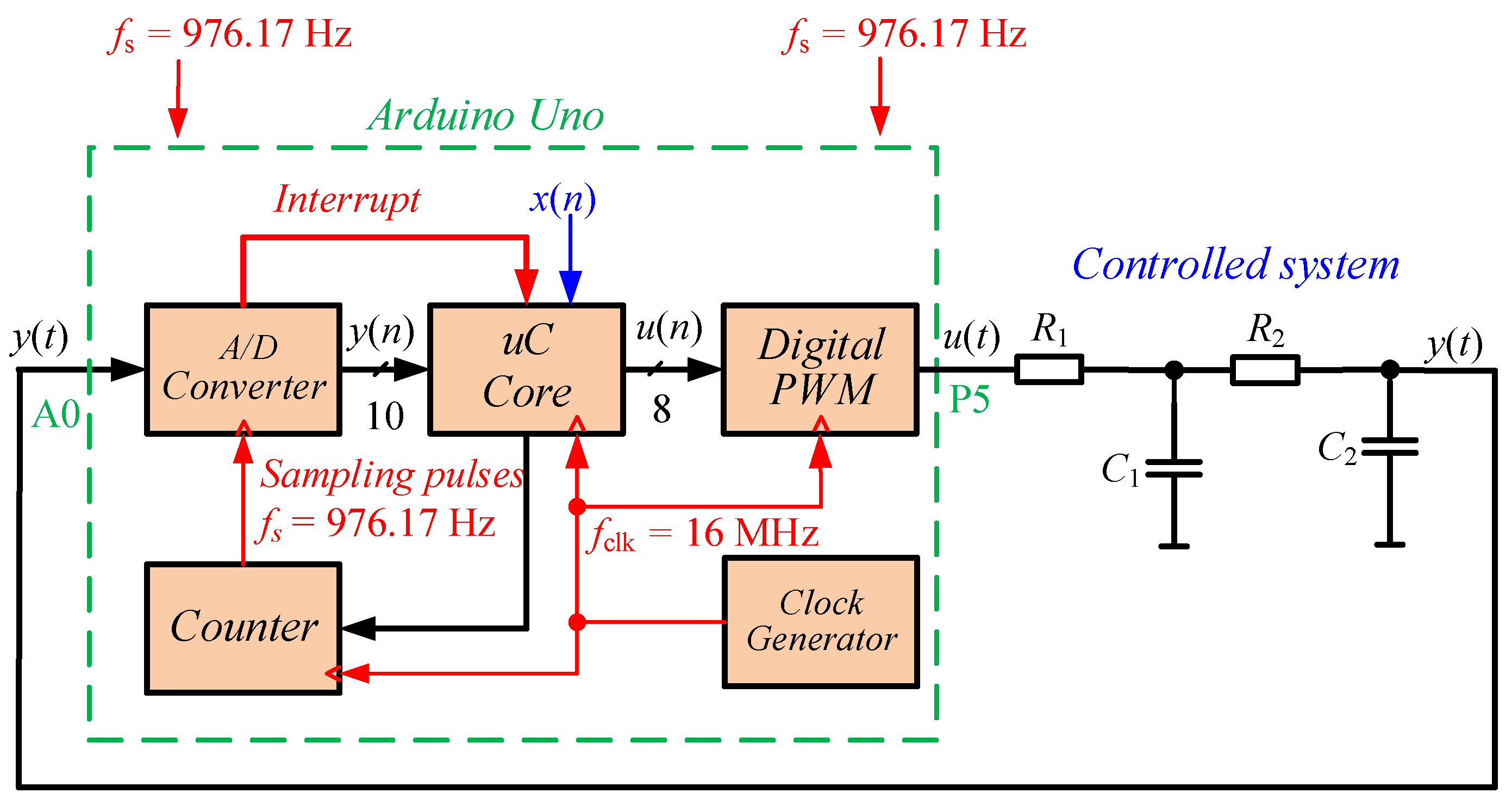
4. Realization of Digital PID Controller Using Arduino Module

The most popular Arduino Uno [7] module was used to implement the digital PID controller. An internal 10-bit A/D converter is used to convert the y(t) signal and a PWM modulator was used as an 8-bit D/A converter to convert the u(t) control variable signal.

The basic source of information about the Arduino system is the webpage arduino.cc [7], but other sites are also worth viewing, for example, Gammon Forum contains a lot of interesting solutions for Arduino modules [37].

In a “standard” C/C++ program, a “main” function should be present. This main function will be called invoked, and from there, one calls up other functions and executes the functionalities of the program. In Arduino, there is no main function. This is replaced by two the functions setup() and loop() [7]. These two functions must be present in every Arduino sketch. Other functions must be created outside the brackets of those two functions. The setup() function will only run once, after each powerup or reset of the Arduino board. It is used to initialize variables, pin modes, start using libraries, etc., whereas function loop() loops consecutively. In the function loop(), the main program should be written, with the understanding that the initialization is already done. In this function, one must always keep in mind that the last line is followed by the first line. In this solution, the frequency of invoking the loop() function depends on its length, and it is also important that this frequency is not constant. Depending on (6) for the calculation of the control variable, there is a sampling period T_s.

As previously mentioned in paragraph 1, all functions found on the page Arduino.cc that implement the digital PID controller are invoked in the loop() function, where a constant sampling period cannot be ensured [15,16,17,18,19,20,21,22,23,24,25,26,27,28,29,37,38,39,40,41,42,43,44,45,46,47,48,49,50,51]. Typically, the period value is determined based on the system time reading. This solution results in a very high-value jitter and worsens the parameter qualities of the processed signals [52,53,54,55,56,57].

To solve this problem, a solution is proposed that provides a constant sampling period of T_s. A sampling period equal to the period of the PWM modulator for pin 5 is assumed, and this period is equal to 1.024 ms. The A/D converter is directly triggered by the microcontroller counter, and an interrupt is generated when the conversion is complete. In this interrupt, the entire algorithm of the regulator is calculated and a new value of u(n) is sent to the PWM modulator. The timing diagram of data flow in the digital PID controller is depicted in Figure 7. The advantage of this solution is that the algorithm of the digital PID controller is calculated every constant period of time.

The block diagram of the controller based on Arduino Uno is depicted in Figure 8. A skeleton version of the program that implements the PID controller is shown in Listing 1, while a detailed version of the program is included in Appendix A. The setup() function includes the initialization of all hardware. The entire program of the PID controller has been placed in the function ISR (ADC_vect), which handles the interrupt generated by the A/D converter. The loop() function, in this case, can be left empty. The ISR (ADC_vect) function can be used instead of loop(), but it must be kept in mind that the time it takes to execute the entire algorithm cannot be longer than the sampling period. Therefore, one should check the execution time with an oscilloscope.

Listing 1. A skeleton version of the program that implements the PID controller.

void   setup()   {      // Pin initialization      // timer initialization      // ADC initialization      // interrupt initialization } ISR   (ADC_vect) // ADC interrupt, fs= 976.165 Hz  {      // ADC reading      // PID controller calculation      // PWM update } EMPTY_INTERRUPT   (TIMER1_COMPB_vect); void   loop()   { // empty main loop  }

Figure 9 shows the time waveform for pin 13 of the microcontroller; it is set to logic one at the beginning of the interrupt handling procedure and reset at the end. It shows that despite the use of a floating point for calculations, the entire interrupt handling procedure takes about one-fifth of the sampling period.

Figure 10 shows a simplified schematic diagram of the experimental control system. In the system, a cascade connection of two RC networks was used as a controlled system. Both networks have the ability to adjust the time constant using potentiometers. Additionally, a second PWM modulator (pin 6) and R₃C₃ network have been used as an additional analog output. In this case, the PWM modulator is used to image the e(t) signal. The view of the control system is shown in Figure 11. It should be noted that the entire system is supplied with a DC voltage of +5 V; therefore, all signals are in the range of 0…+5 V.

An example of experimental time waveforms using a PI controller (closed-loop) with a first-order object for a step change of setpoint x(t) from 0.2 to 0.8 is shown in Figure 12, which shows the time waveforms of the controller error e(t) and the measured value of the process y(t).

By modifying the program from Listing A1, it can also be used to identify the parameters of the controlled system; for example, performing a test for a step response of an open-loop system.

For programming and debugging, the typical Arduino IDE 2 (Integrated Development Environment) is used. Among the many useful features of this environment, the Serial Plotter function should be mentioned [7]. It allows us to visualize the variables sent by the serial port. Figure 13 shows the step response of the controlled system. With the Serial Plotter function, it is possible to test the control systems without an oscilloscope. A skeleton version of the program for Serial Plotter visualization of the open-loop system step response is described in Listing 2.

Listing 2. A skeleton version of the program for Serial Plotter visualization of the open-loop system step response.

// fsk – Serial Plotter sampling frequency #define fsk 10 const   float fs=976.165; // sampling frequency const   int Nk=fs/fsk; ISR   (ADC_vect) // ADC interrupt, fs= 976.165 Hz  {      // ADC reading      U=1;      // PWM update      if (counter++>Nk) {      Serial.println(y);      counter=0;      } }

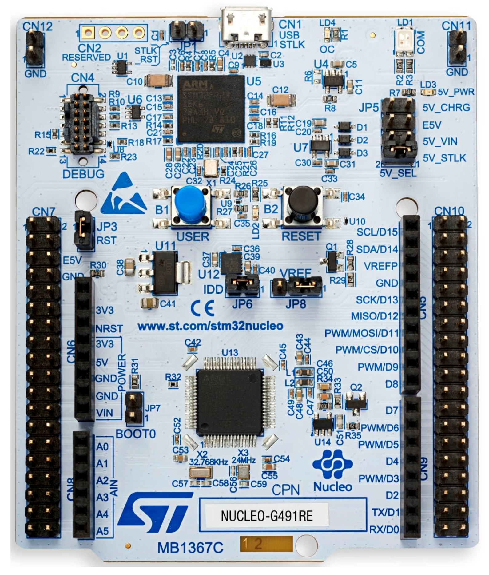
5. Realization of Digital PID Controller Using STM32G491RE-Nucleo

The STM32 family of 32-bit microcontrollers is based on the ARM Cortex^®-M processor from the STMicroelectronics company. STM32 microcontrollers combine very high performance, real-time capabilities, digital signal processing, low power and connectivity, while maintaining full integration and ease of development [10].

The company’s offer includes a whole range of development boards [10]. A low-cost module equipped with a 12-bit A/D converter and a 12-bit D/A converter, STM32G491RE-Nucleo, was chosen to implement the digital PID controller. The STM32 Nucleo-64 development board with STM32G491RE microcontroller supports Arduino and ST morpho connectivity [10,58]. Figure 14 shows the view of the STM32G491RE-Nucleo board.

For programming and debugging, the typical STM32CubeIDE ver. 1.11.2. (Integrated Development Environment) is used. STM32Cube includes STM32CubeMX, a graphical software configuration tool that allows the generation of C initialization code using graphical wizards, according to the hardware configuration of our board. For example, if we have the STM32G491RE-Nucleo, which is based on the STM32G491RE microcontroller, and we want to use its user LED (marked as LD2 on the board), then STM32CubeMX will automatically generate all source files containing the C code required to configure the microcontroller (clock, peripheral ports, and so on) and the GPIO connected to the LED.

The block diagram of the digital PID controller based on STM32G491RE-Nucleo is depicted in Figure 15. The microcontroller is powered by +3.3 V, so all signals in the system are in the range of 0… +3.3 volts.

As in the case of the implementation of the digital controller using Arduino, the entire algorithm is executed when handling the interrupt from the A/D converter. Due to the assumed sampling frequency of f_s = 10 kHz, the time available for calculations is less than 100 µs. A timing diagram of data flow in the digital PID controller based on STM32G491RE-Nucleo is shown in Figure 16.

The following is a list of hardware initialization of the digital PID controller based on STM32G491RE for STM32CubeMX during the generation of C initialization code:

• Initialization of A/D converter—single-ended input pin PA0, Triger Conversion Source, Timer 3, Triger Out event, ADC1 and ADC2 global interrupt;
• GPIO—GPIO_Output PA10, Output Push Pull;
• D/A converter—OUT1 mode, Connected to external pin only;
• Timer 3—Clock source, Internal Clock, Channel1, Output Compare No Output, Counter period, 16000-1, auto-reload preload, enable, Trigger Event Selection TRGO—Update Event;
• Initialization of interrupt system.

The STM32CubeMX interface for pin assignment of the STM32G491RE microcontroller is depicted in Figure 17.

As with Arduino, a digital PID controller has been implemented. A simplified skeleton version of the program that implements the PID controller is shown in Listing 3. However, it should be noted that using the STM32CubeMX development environment is more complex than in the case of Arduino, and despite creating precise instructions on how to configure the microcontroller, it sometimes causes problems for students. Unfortunately, the listing of such a program containing the necessary initialization of the microcontroller hardware is several pages long, and it is easy to get lost in it.

Listing 3. A simplified skeleton version of the program that implements the PID controller.

// // Global variable initialization Int   main(void)    {     // Pin initialization     // timer initialization     // ADC initialization     // interrupt initialization     /* Infinite loop */     while (1)     {     // empty loop     } } Void   HAL_ADC_ConvCpltCallback(ADC_HandleTypeDef *hadc)  // ADC interrupt, fs= 10kHz  {      // ADC reading      // PID controller calculation      // DAC update }

Figure 18 shows the time waveforms for the case of processing a sinusoidal input signal y(t) with a frequency of 1 kHz and an amplitude of 1 V (the input signal has a +1.5 V offset) to an analog output u(t).

As in the case of the Arduino module, the program has been modified to determine the step response of the open-loop system. The open-loop step response of the second-order object is depicted in Figure 19. If the student does not have an oscilloscope, the capabilities of the Development Environment STM32CubeIDE can be used for imaging variables y(n).

Examples of experimental time waveforms of a PI controller (closed-loop) with a second-order object for a step change of setpoint x(t) from 0.2 to 0.7 are shown in Figure 20, Figure 21 and Figure 22. They show the time waveforms of the control variable u(t) and the measured value of the process y(t) for different controller parameters.

6. Tuning the PID Controller

After successfully implementing a digital PID controller, the first question is how to tune a PID controller. That is, what should be the values of the three basic parameters of the regulator k_c, T_i and T_d. Probably the first, and certainly the best known, are the Zeigler–Nichols rules. Published in 1942 [59], Zeigler and Nichols described two methods of tuning a PID loop. Over several decades of using regulators, many rules have been created to address the question of how to tune a PID controller. This problem is so ubiquitous that thousands of publications on this subject can be found in the literature [30,31,32,33,34,54,60]. The description of even the most important ones would exceed the scope of this publication many times, which is why only one very simple method will be presented.

One of the simpler methods of determining digital PID controller parameters is the method called Direct Synthesis tuning rules [61], based on first-order model approximation. In this method, it is necessary to know the gain of the object in the open loop k_p and the time constant τ_p. The excitation value of the regulator k_c is determined from the equation

$$k_c=\frac{1}{k_p{\tau }_{ratio}}$$

(14)

where τ_ratio defines the speed of response.

While the value of the integral time T_i parameter is τ_p, the value of derivative time T_d = 0. Depending on the requirements, the value of τ_ratio is selected from the range 1 to 4. For a value of 1, the response of a closed system will be the fastest, and for a value of 4, the response will be the slowest. For the control objects under consideration, the usefulness of this method has been confirmed in practice.

7. Students Tasks

The primary purpose of the automatic control laboratories is to provide students enrolled in the fundamental automatic control course with a practical understanding of feedback control principles, especially in the real-time process. Through hands-on experimentation, students will learn how to determine the dynamic properties of real systems and adjust the PID controllers accordingly. It is possible to find examples of laboratory tasks on the web pages of many universities, for example [62,63,64], or in some papers [44,45,46,47,48,49,50,51], [65,66,67,68,69].

Typically, student assignments are divided into five basic stages: identification of the process, calculation of the PID controller parameters, implementation of the PID controller, testing of the closed-loop with PID controller, and analysis of the results.

7.1. Identification of the Process

At the beginning of the laboratory exercise, the task of students is to identify the parameters of the tested object, which are determined by the gain of the object in the open-loop k_p and the time constant τ_p, and time delay τ_d. These parameters are determined from a unit-step response of the process. Examples of object step responses are shown in Figure 13 and Figure 19.

My didactic practice shows that in order to deepen the knowledge of students, it is required that they also implement a simple hysteresis regulator, as shown in Figure 23. Examples of waveforms for such a controller are shown in Figure 24.

7.2. Calculation of the PID Controller Parameters

In the next step, the student’s task is to calculate the values of the PID controller parameters k_c, k_i and k_d for the given control parameters and the selected method. They are also encouraged to check the obtained results by performing simulation tests, for example using Matlab or Matlab-Simulink.

7.3. The PID Controller Implementation

The PID controller is implemented by students based on algorithms presented in Section 2, Section 3, Section 4 and Section 5. Students are also encouraged to create their implementations of the PID controller. For the more talented students, it is recommended they implement the PID controller with autotuning.

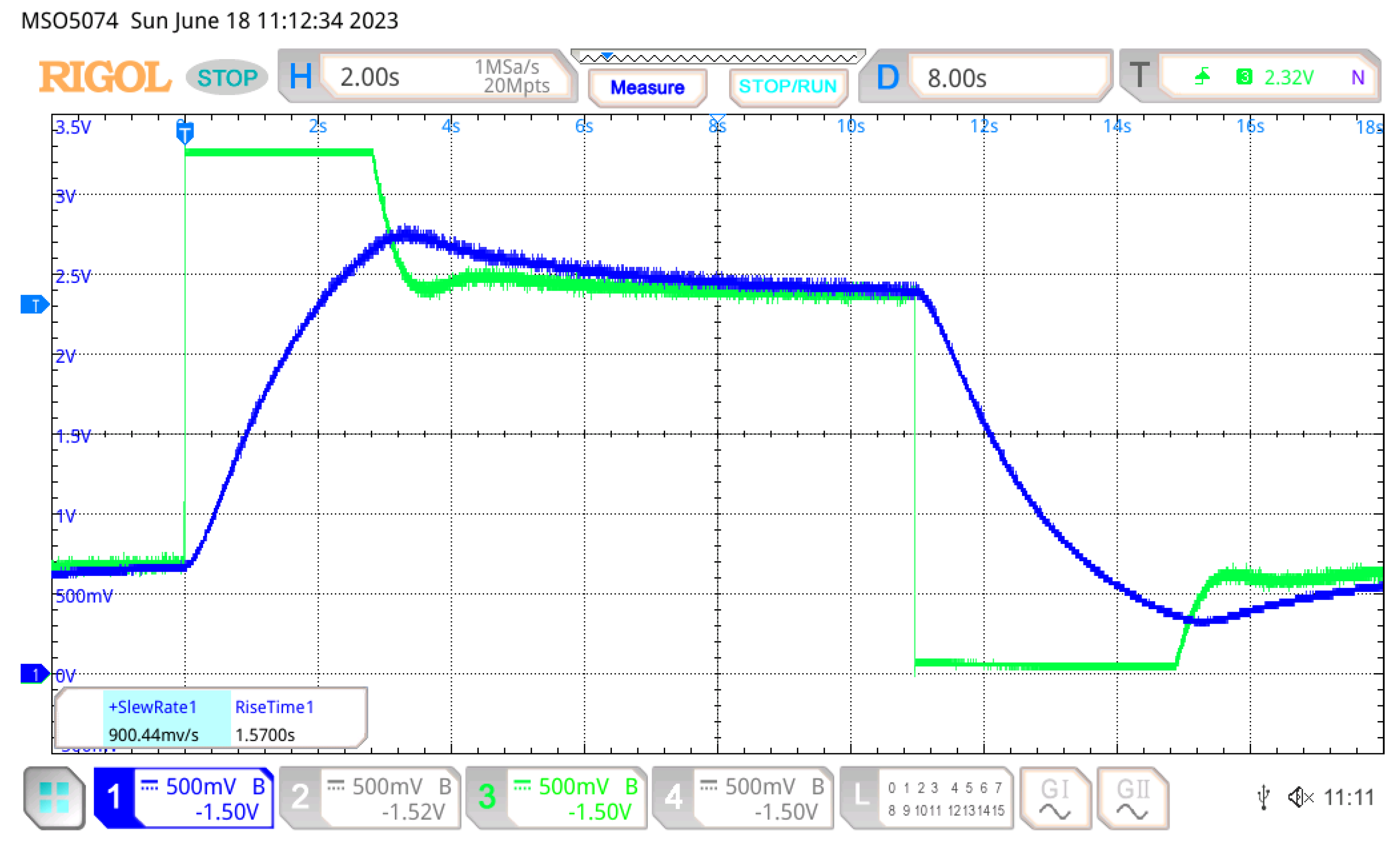
7.4. Testing of Close Loop with PID Controller

During the tests of the closed-loop system, the quality parameters of the regulation are examined, such as rise time, overshoot, settling time, steady-state error, stability, etc. Typically, these parameters are determined from a unit-step response of a closed-loop system.

7.5. Analysis of the Results

Finally, students are required to prepare a written report on the research carried out and an analysis of the research results obtained.

The solutions presented in the paper have been successfully tested in practice during distance learning during the COVID-19 pandemic. These methods were used during the distance learning of the classes in Design of Industrial Control Systems, Digital Signal Processors and Microcontrollers, and Foundations of Digital and Microprocessor Engineering, and they were successfully used by over one hundred graduate or undergraduate students. Currently, these laboratory tasks are conducted under on-site conditions.

The laboratory also serves students specializing in systems identification, providing them with practical experience in evaluating the strengths and weaknesses of various methods for modeling real dynamic systems.

In addition to regular instruction, the automatic control laboratory continuously supports master’s and bachelor’s thesis research, as well as student projects.

8. Conclusions

In the paper, the original implementation of the digital PID controller using the most popular and simple Arduino Uno module is presented. The developed systems are a cheap alternative to more expensive professional systems designed for the implementation of control systems.

The proposed system removes the main disadvantage of the available implementations of the digital PID controller for Arduino modules, which is the variable sampling period. The advantage of this solution is that the algorithm of the digital PID controller is calculated every constant period of time. An identical solution was presented for STM32 modules on the example of the STM32G491RE module.

Of course, the solutions shown in the paper can be successfully used to test other control algorithms. For example, both implementations of Arduino and STM32 were used to test the control system with a hysteresis regulator.

When using Arduino Uno modules with an 8-bit AVR microcontroller, it can only be used to control slow-variable processes with a time constant of the order of seconds. However, when using STM32 modules, the capabilities of ARM processors are much greater, and they can be applied to objects with a time constant of milliseconds.

It should be emphasized that using the Arduino IDE development environment is very simple and does not cause problems for students.

Both the solutions presented in the paper have been successfully tested in practice by students during remote learning during the COVID-19 pandemic. It should be noted that even after the end of the pandemic, the developed solutions remain very useful in the process of teaching students automatic control techniques.

The solutions presented in the paper can also be successfully applied to other applications, such as motor control, digital signal processing, power electronics, etc.

References

1. National Instruments, myRIO. Available online: https://www.ni.com/pl-pl/shop/hardware/products/myrio-student-embedded-device.html (accessed on 13 June 2023).
2. Speedgoat. Available online: https://www.speedgoat.com (accessed on 13 June 2023).
3. 8-Bit AVR MCUs, Microchip. Available online: https://www.microchip.com/en-us/products/microcontrollers-and-microprocessors/8-bit-mcus/avr-mcus (accessed on 13 June 2023).
4. ARM MCUs, ARM. Available online: https://www.arm.com/ (accessed on 13 June 2023).
5. C2000 Real-Time Microcontrollers, Texas Instruments. Available online: https://www.ti.com/microcontrollers-mcus-processors/c2000-real-time-control-mcus/overview.html (accessed on 13 June 2023).
6. ADUC84x MCUs. Available online: https://www.analog.com/en/index.html (accessed on 13 June 2023).
7. Arduino. Available online: https://www.arduino.cc/ (accessed on 13 June 2023).
8. Raspberry Pi. Available online: https://www.raspberrypi.org/ (accessed on 13 June 2023).
9. BeagleBone. Available online: https://beagleboard.org/black (accessed on 13 June 2023).
10. STM32 32-Bit Arm Cortex MCUs, STMicroelectronics. Available online: https://www.st.com/en/microcontrollers-microprocessors/stm32-32-bit-arm-cortex-mcus.html (accessed on 13 June 2023).
11. Available online: https://www.microchip.com/en-us/products/microcontrollers-and-microprocessors (accessed on 1 July 2023).
12. Available online: https://mu.microchip.com/ (accessed on 1 July 2023).
13. Available online: https://mu.microchip.com/rapid-prototyping-with-the-curiosity-nano-platform (accessed on 1 July 2023).
14. Ghassoul, M. Design of Three-Term Controller Using a PIC18F452 Microcontroller. In Renewable Energy; Taner, T., Tiwari, A., Ustun, T., Eds.; IntechOpen: Rijeka, Croatia, 2020; Chapter 17. [Google Scholar] [CrossRef] [Green Version]
15. Sun, L.; You, F. Machine Learning and Data-Driven Techniques for the Control of SmartPower Generation Systems: An Uncertainty Handling Perspective. Engineering 2021, 7, 1239–1247. [Google Scholar] [CrossRef]
16. Beauregard, B. PID Controller, Arduino, PID-1.2.0.zip. Available online: https://www.arduino.cc/reference/en/libraries/pid/ (accessed on 1 April 2023).
17. Daniel, PID Controller, Arduino, PIDController-0.0.1.zip. Available online: https://www.arduino.cc/reference/en/libraries/pidcontroller/ (accessed on 1 April 2023).
18. Tillaart, R. PID_RT, Arduino, PID_RT-0.1.6.zip. Available online: https://www.arduino.cc/reference/en/libraries/pid_rt/ (accessed on 1 April 2023).
19. Pribičević, Z. mrm-pid, Arduino, mrm_pid-0.0.4.zip. Available online: https://www.arduino.cc/reference/en/libraries/mrm-pid/ (accessed on 1 April 2023).
20. Falcons, A. Custom PID, Arduino, Custom_PID-1.0.0.zip. Available online: https://www.arduino.cc/reference/en/libraries/custom-pid/ (accessed on 1 April 2023).
21. Beauregard, B. PID_v2, Arduino, PID_v2-2.0.1.zip. Available online: https://www.arduino.cc/reference/en/libraries/pid_v2/ (accessed on 1 April 2023).
22. Adjal, A. Embedded Type-C PID, Arduino, Embedded_Type_C_PID-1.1.3.zip. Available online: https://www.arduino.cc/reference/en/libraries/embedded-type-c-pid/ (accessed on 1 April 2023).
23. Forrest, D. PID_v1_bc, Arduino, PID_v1_bc-1.2.7.zip. Available online: https://www.arduino.cc/reference/en/libraries/pid_v1_bc/ (accessed on 1 April 2023).
24. Thomas, K. PID Controllers Modular Professional Arduino, PID_Controllers_Modular_Professional-1.0.2.zip. Available online: https://www.arduino.cc/reference/en/libraries/pid-controllers-modular-professional/ (accessed on 1 April 2023).
25. Lloyd, D. QuickPID, Arduino, QuickPID-3.1.8.zip. Available online: https://www.arduino.cc/reference/en/libraries/quickpid/ (accessed on 1 April 2023).
26. Matera, M. FastPID, Arduino, FastPID-1.3.1.zip. Available online: https://www.arduino.cc/reference/en/libraries/fastpid/ (accessed on 1 April 2023).
27. cjmccjmccjmc, ControlLoop, Arduino, ControlLoop-1.0.2.zip. Available online: https://www.arduino.cc/reference/en/libraries/controlloop/ (accessed on 1 April 2023).
28. Downing, R. AutoPID, Arduino, AutoPID-1.0.3.zip. Available online: https://www.arduino.cc/reference/en/libraries/autopid/ (accessed on 1 April 2023).
29. Bruere-Terreault, J. TimedPID, Arduino, TimedPID-1.0.0.zip. Available online: https://www.arduino.cc/reference/en/libraries/timedpid/ (accessed on 1 April 2023).
30. Astrom, K.J.; Wittenmark, B. Computer-Controlled System, Theory and Design, 3rd ed.; Prentice Hall, Inc.: Englewood Cliffs, NJ, USA, 2013. [Google Scholar]
31. Williamson, D. Digital Control and Implementation; Prentice Hall, Inc.: Englewood Cliffs, NJ, USA, 1991. [Google Scholar]
32. Stokes, J.; Sohie, G.R.L. Implementation of PID Controllers on the Motorola DSP56000/DSP56001; Motorola Digital Signal Processors, APR5.pdf; Motorola: Schaumburg, IL, USA, 1996. [Google Scholar]
33. Ahmed, I. Implementation of PID and Deadbeat Controllers with the TMS320 Family; Application Report: SPRA083.pdf; Texas Instruments: Dallas, TX, USA, 1997. [Google Scholar]
34. Aström, K.J.; Murray, R.M. Feedback Systems; Princeton University Press: Princeton, NJ, USA, 2009. [Google Scholar]
35. Sallen, R.P.; Key, E.L. A Practical Method of Designing RC Active Filters. IRE Trans. Circuit Theory 1955, 2, 74–85. [Google Scholar] [CrossRef]
36. Karki, J. Active Low-Pass Filter Design; Application Note, SLOA049D; Texas Instruments: Princeton, NJ, USA, 2023. [Google Scholar]
37. Gammon Forum. Available online: https://gammon.com.au/forum/index.php?bbtopic_id=123 (accessed on 1 July 2023).
38. Catalbas, B.; Uyanik, I. A Low-cost Laboratory Experiment Setup for Frequency Domain Analysis for a Feedback Control Systems Course. IFAC PapersOnLine 2017, 50, 15704–15709. [Google Scholar] [CrossRef]
39. Li, J.H. Control System Laboratory with Arduino. In Proceedings of the 2018 International Symposium on Computer, Consumer and Control (IS3C), Taichung, Taiwan, 6–8 December 2018; pp. 181–184. [Google Scholar] [CrossRef]
40. Alleyne, A.G.; Block, D.J.; Meyn, S.P.; Perkins, W.R.; Spong, M.W. An interdisciplinary, interdepartmental control systems laboratory. IEEE Control Syst. Mag. 2005, 25, 50–55. [Google Scholar] [CrossRef]
41. Jitthammapirom, P.; Chayratsami, P.; Somha, W. Development of Remote Laboratory for Feedback Control System Class. In Proceedings of the 2021 6th International STEM Education Conference (iSTEM-Ed), Pattaya, Thailand, 10–12 November 2021; pp. 1–4. [Google Scholar] [CrossRef]
42. McLoone, S.C.; Maloco, J. A cost-effective hardware-based laboratory solution for demonstrating PID control. In Proceedings of the 2016 UKACC 11th International Conference on Control (CONTROL), Belfast, UK, 29 August 2016; pp. 1–6. [Google Scholar] [CrossRef]
43. Khan, I.; Żmuda, M.; Konopka, P.; Gustavsson, I.; Håkansson, L. Enhancement of remotely controlled laboratory for Active Noise Control and acoustic experiments. In Proceedings of the 2014 11th International Conference on Remote Engineering and Virtual Instrumentation (REV), Porto, Portugal, 26–28 February 2014; pp. 285–290. [Google Scholar] [CrossRef]
44. Shoureshi, R. A course on microprocessor-based control systems. IEEE Control Syst. Mag. 1992, 12, 39–42. [Google Scholar] [CrossRef]
45. Li, X.; Yu, H.; Zeng, P.; Zang, C.; Sun, L.; Yuan, M. A design method of optimal PI controller with saturation characteristic for second-order processes. In Proceedings of the 2015 IEEE International Conference on Cyber Technology in Automation, Control, and Intelligent Systems (CYBER), Shenyang, China, 8–12 June 2015; pp. 1634–1639. [Google Scholar] [CrossRef]
46. Zhou, L.; Ma, A.; Liu, L.; Zhu, N. The analysis of optimal sampling period on output multi-rate predictive control system. In Proceedings of the 2010 Chinese Control and Decision Conference, Xuzhou, China, 26–28 May 2010; pp. 1102–1105. [Google Scholar] [CrossRef]
47. Huba, M.; Chamraz, S.; Bistak, P.; Vrancic, D. Making the PI and PID Controller Tuning Inspired by Ziegler and Nichols Precise and Reliable. Sensors 2021, 21, 6157. [Google Scholar] [CrossRef] [PubMed]
48. Ho, T.-J.; Chang, C.-H. Robust Speed Tracking of Induction Motors: An Arduino-Implemented Intelligent Control Approach. Appl. Sci. 2018, 8, 159. [Google Scholar] [CrossRef] [Green Version]
49. Meng, Z.; Zhang, L.; Li, H.; Zhou, R.; Bu, H.; Shan, Y.; Ma, X.; Ma, R. Design and Application of Liquid Fertilizer pH Regulation Controller Based on BP-PID-Smith Predictive Compensation Algorithm. Appl. Sci. 2022, 12, 6162. [Google Scholar] [CrossRef]
50. Zarzycki, K.; Ławryńczuk, M. Fast Real-Time Model Predictive Control for a Ball-on-Plate Process. Sensors 2021, 21, 3959. [Google Scholar] [CrossRef] [PubMed]
51. de Moura Oliveira, P.B.; Hedengren, J.D.; Solteiro Pires, E.J. Swarm-Based Design of Proportional Integral and Derivative Controllers Using a Compromise Cost Function: An Arduino Temperature Laboratory Case Study. Algorithms 2020, 13, 315. [Google Scholar] [CrossRef]
52. Sozanski, K. Digital Signal Processing in Power Electronics Control Circuits, 2nd ed.; Springer: London, UK, 2017. [Google Scholar]
53. Azeredo-Leme, C. Clock jitter effects on sampling: A tutorial. IEEE Circuits Syst. Mag. 2011, 3, 26–37. [Google Scholar] [CrossRef]
54. Brannon, B. Sampled Systems and the Effects of Clock Phase Noise and Jitter; Application Note AN-756, Technical Report; Analog Devices, Inc.: Norwood, MA, USA, 2004. [Google Scholar]
55. Brannon, B.; Barlow, A. Aperture Uncertainty and ADC System Performance; Application Note AN-501, Technical Report; Analog Devices, Inc.: Norwood, MA, USA, 2006. [Google Scholar]
56. Redmayne, D.; Trelewicz, E.; Smith, A. Understanding the Effect of Clock Jitter on High Speed ADCs; Design Note 1013, Technical Report; Linear Technology, Inc.: Milpitas, CA, USA, 2006. [Google Scholar]
57. Mota, M. Understanding Clock Jitter Effects on Data Converter Performance and How to Minimize Them; Technical Report; Synopsis Inc.: Mountain View, CA, USA, 2010. [Google Scholar]
58. Noviello, C. Mastering STM32, 2nd ed.; Leanpub: Victoria, BC, Canada, 2022; Available online: https://leanpub.com/mastering-stm32-2nd (accessed on 18 July 2023).
59. Ziegler, J.G.; Nichols, N.B. Optimum Settings for Automatic Controllers. Trans. ASME 1942, 64, 759–768. [Google Scholar] [CrossRef]
60. O’Dwyer, A. Handbook of PI and PID Controller Tuning Rules, 3rd ed.; Imperial College Press: London, UK, 2009. [Google Scholar]
61. Starr, K.D. Single Loop Control Methods; ABB: Zurich, Switzerland, 2015. [Google Scholar]
62. Control Laboratory, RWTH Aachen University. Available online: https://www.irt.rwth-aachen.de/cms/IRT/Studium/Lehre-Bachelor/~jdce/Regelungstechnisches-Labor/?lidx=1 (accessed on 18 July 2023).
63. Automatic Control, Lund University. Available online: https://www.control.lth.se/ (accessed on 18 July 2023).
64. Control Tutorials, University of Michigan. Available online: https://ctms.engin.umich.edu/CTMS/index.php?aux=Home (accessed on 18 July 2023).
65. Wilson, D. Teaching Your PI Controller to Behave; Texas Instruments: Dallas, TX, USA, 2015; Available online: https://e2e.ti.com/blogs_/b/industrial_strength/posts/teaching-your-pi-controller-to-behave-part-i (accessed on 18 July 2023).
66. Mohammed, A.K.; Zoghby HM El Elmesalawy, M.M. Remote Controlled Laboratory Experiments for Engineering Education in the Post-COVID-19 Era: Concept and Example. In Proceedings of the 2020 2nd Novel Intelligent and Leading Emerging Sciences Conference (NILES), Giza, Egypt, 24–26 October 2020; pp. 629–634. [Google Scholar] [CrossRef]
67. Uğur, M.; Savaş, K.; Erdal, H. An internet-based real-time remote automatic control laboratory for control education. Procedia Soc. Behav. Sci. 2010, 2, 5271–5275. [Google Scholar] [CrossRef] [Green Version]
68. Rossiter, J.A.; Dormido, S.; Vlacic, L.; Jones, B.L.; Murray, R.M. Opportunities and good practice in control education: A survey. IFAC Proc. Vol. 2014, 47, 10568–10573. [Google Scholar] [CrossRef]
69. Barber, R.; Horra, M.; Crespo, J. Control Practices using Simulink with Arduino as Low Cost Hardware. IFAC Proc. Vol. 2013, 46, 250–255. [Google Scholar] [CrossRef]
Figure 1. A feedback loop with standard analog PID controller.
Electronics 12 03235 g001
Figure 2. The block diagram of the digital PID controller.
Electronics 12 03235 g002
Figure 3. The block diagram of the digital PID controller with saturation, and with the PWM modulator on the output.
Electronics 12 03235 g003
Figure 4. The block diagram of the digital PID controller with modified derivative term connection.
Electronics 12 03235 g004
Figure 5. Second-order passive controlled system simulator.
Electronics 12 03235 g005
Figure 6. Second-order active controlled system simulator.
Electronics 12 03235 g006
Figure 7. Timing diagram of data flow in the digital PID controller.
Electronics 12 03235 g007
Figure 8. The block diagram of controller based on Arduino Uno.
Electronics 12 03235 g008
Figure 9. Time waveform of pin 13, Arduino UNO, A/D interrupt, 976.76 Hz.
Electronics 12 03235 g009
Figure 10. A simplified schematic diagram of the experimental control system.
Electronics 12 03235 g010
Figure 11. The view of the control system.
Electronics 12 03235 g011
Figure 12. Time waveforms of the PI controller, closed-loop step response of first-order object, e(t)—green, y(t)—red, for x(t) = 0.2 → 0.8, Ti = 3.0, kc = 2.0.
Electronics 12 03235 g012
Figure 13. Time waveform of step response of second-order controlled system y(t), drawn by Serial Plotter for fsk = 10 Hz.
Electronics 12 03235 g013
Figure 14. A view of the STM32G491RE-Nucleo module.
Electronics 12 03235 g014
Figure 15. The block diagram of the digital PID controller based on STM32G491RE-Nucleo.
Electronics 12 03235 g015
Figure 16. Timing diagram of data flow in the digital PID controller based on STM32G491RE-Nucleo.
Electronics 12 03235 g016
Figure 17. STM32CubeMX interface for pin assignment of the STM32G491RE microcontroller.
Electronics 12 03235 g017
Figure 18. Time waveforms of the STM32G491RE-Nucleo module, y(t) orange curve, u(t) blue curve.
Electronics 12 03235 g018
Figure 19. Time waveforms of the open-loop step response of the second-order object, u(t)—green, y(t)—blue.
Electronics 12 03235 g019
Figure 20. Time waveforms of the PI controller, closed-loop step response of second-order object, u(t)—green, y(t)—blue, for x(t) = 0.2 → 0.7, Ti = 3.0, kc = 1.0.
Electronics 12 03235 g020
Figure 21. Time waveforms of the PI controller, closed-loop step response of second-order object, u(t)—green, y(t)—blue, x(t) = 0.2 → 0.7, Ti = 0.5, kc = 2.0.
Electronics 12 03235 g021
Figure 22. Time waveforms of the PI controller, closed-loop step response of second-order object, u(t)—green, y(t)—blue, x(t) = 0.2 → 0.7, Ti = 3.0, kc = 5.0.
Electronics 12 03235 g022
Figure 23. The block diagram of the hysteresis controller based on Arduino Uno.
Electronics 12 03235 g023
Figure 24. Time waveforms of the hysteresis controller, closed-loop step response of the first-order object, u(t)—green, y(t)—purple.
Electronics 12 03235 g024
Disclaimer/Publisher’s Note: The statements, opinions and data contained in all publications are solely those of the individual author(s) and contributor(s) and not of MDPI and/or the editor(s). MDPI and/or the editor(s) disclaim responsibility for any injury to people or property resulting from any ideas, methods, instructions or products referred to in the content.