
Lightweight Tunnel Defect Detection Algorithm Based on Knowledge Distillation

Abstract
:1. Introduce
- (1)
- Create a deep pooling residual structure to pool and weight feature information deeply
- (2)
- Use MobileNetv3 to optimize the network backbone for improved model lightweight
- (3)
- Construct a method for multidimensional knowledge extraction that can extract information from both the feature layer and the output layer.
2. Related Work
2.1. YOLO Method
2.2. Knowledge Distillation
3. Improving the Model
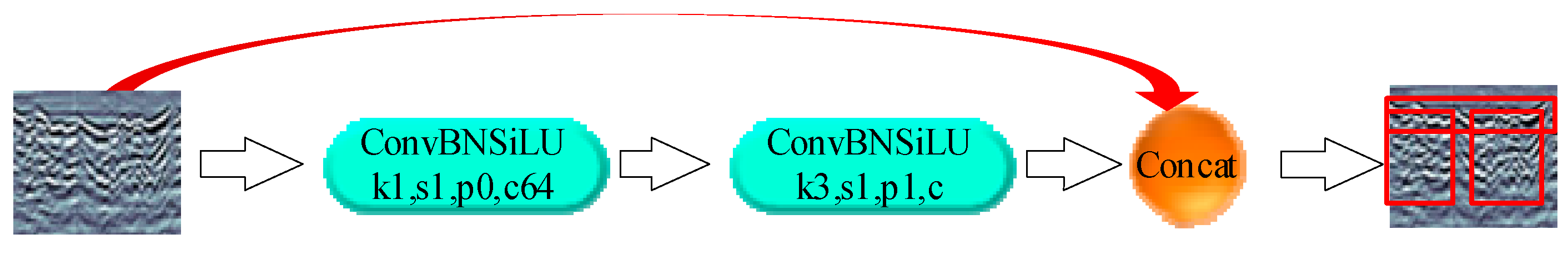
3.1. Deep Pooling of Residual Structures
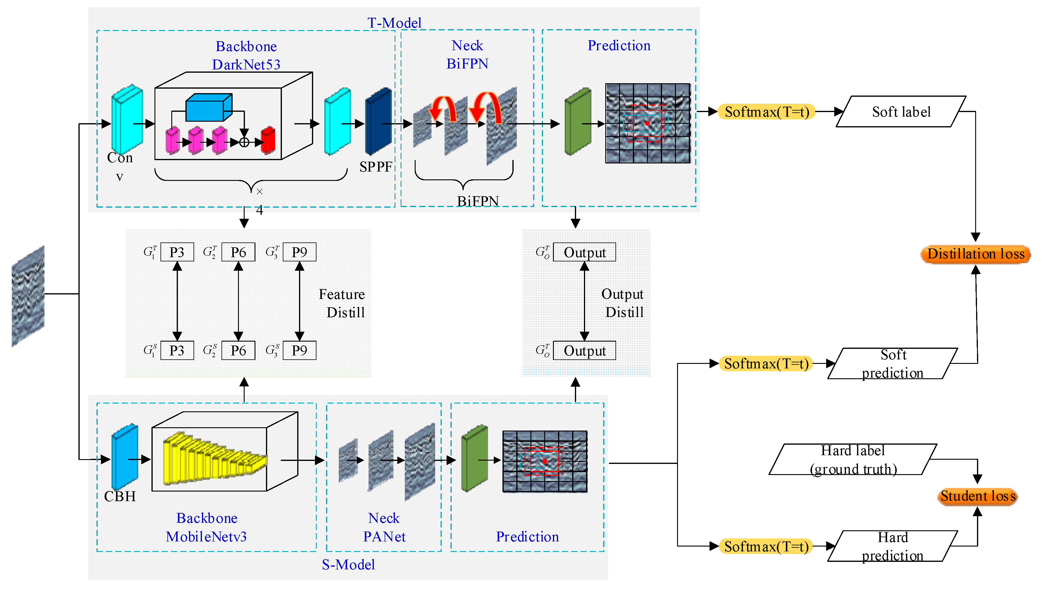
3.2. Multidimensional Knowledge Distillation
4. Experimental Studies
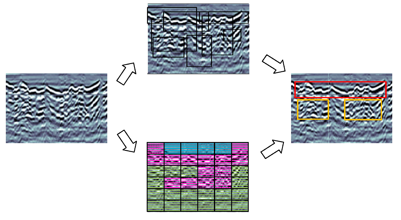
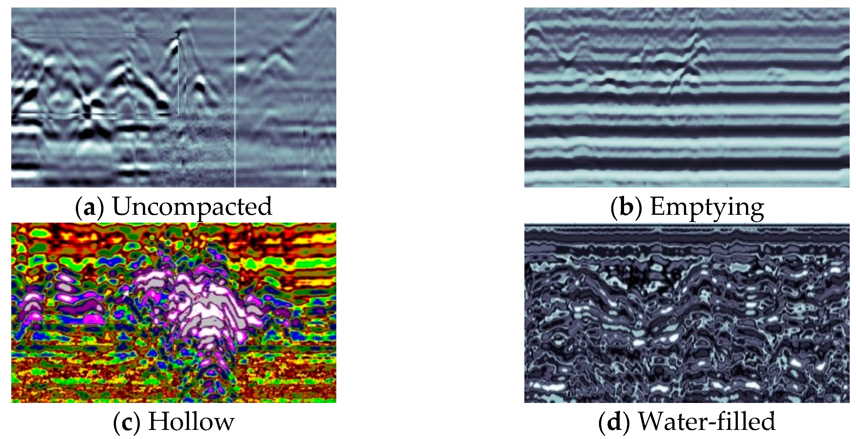
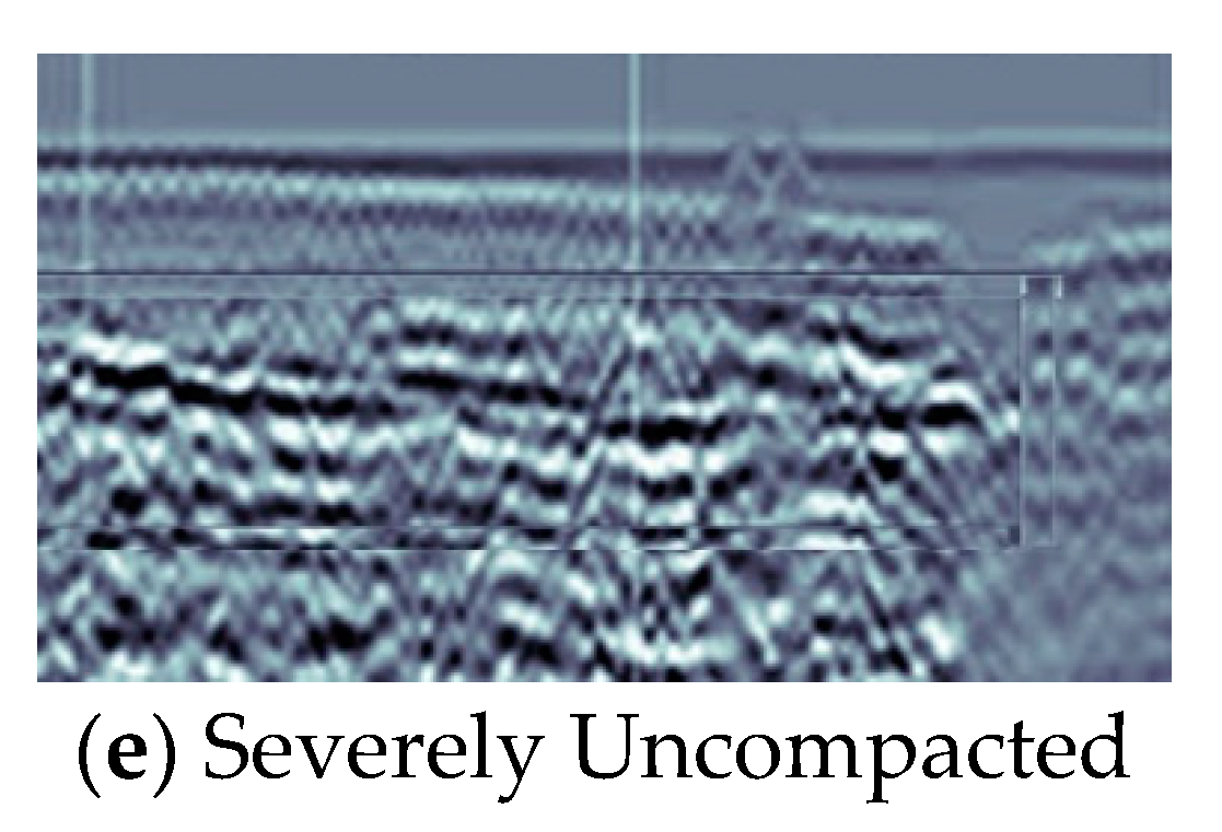
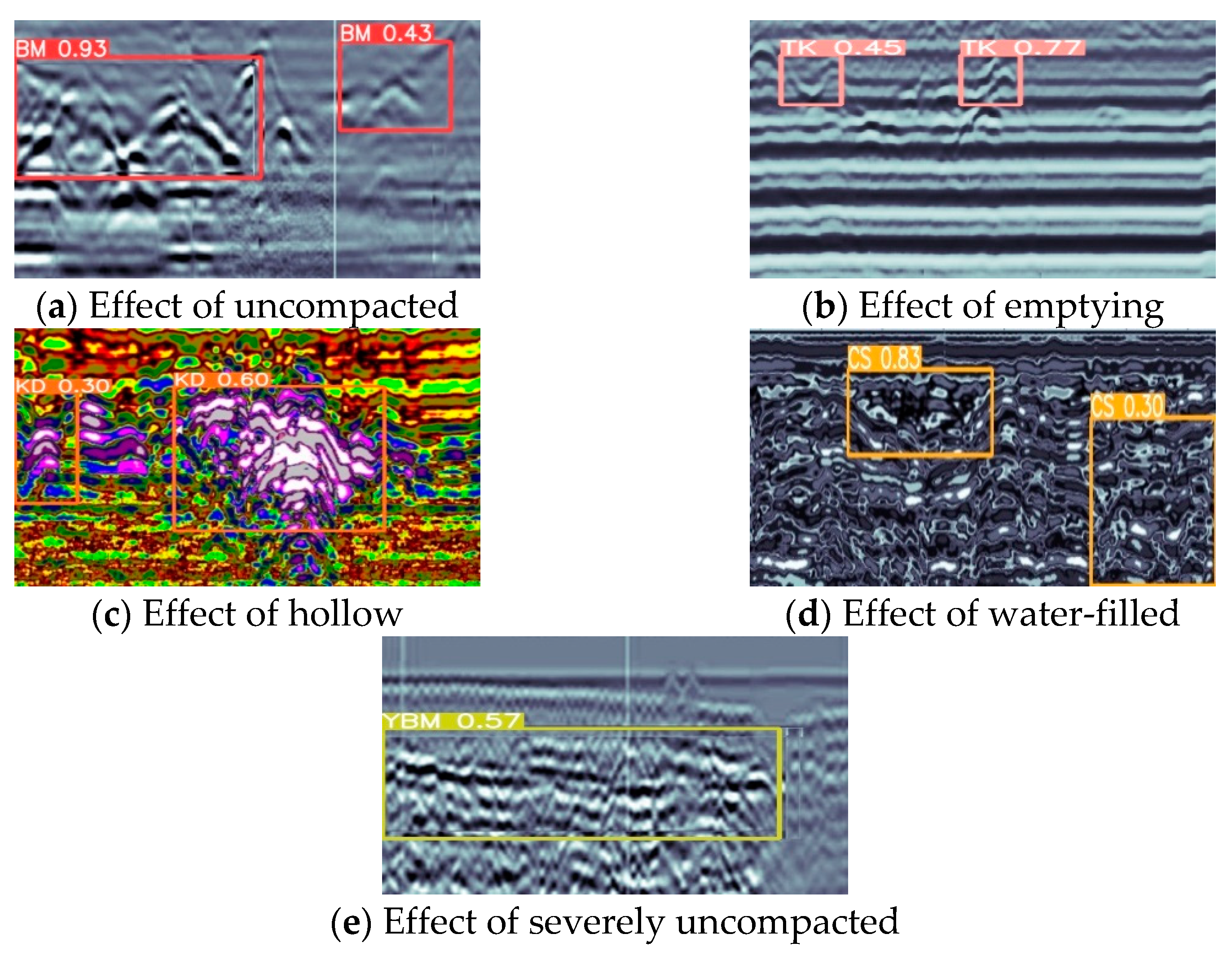
4.1. Data Processing
4.2. Experimental Procedure
4.2.1. Experimental Configuration
4.2.2. Evaluation Indicators
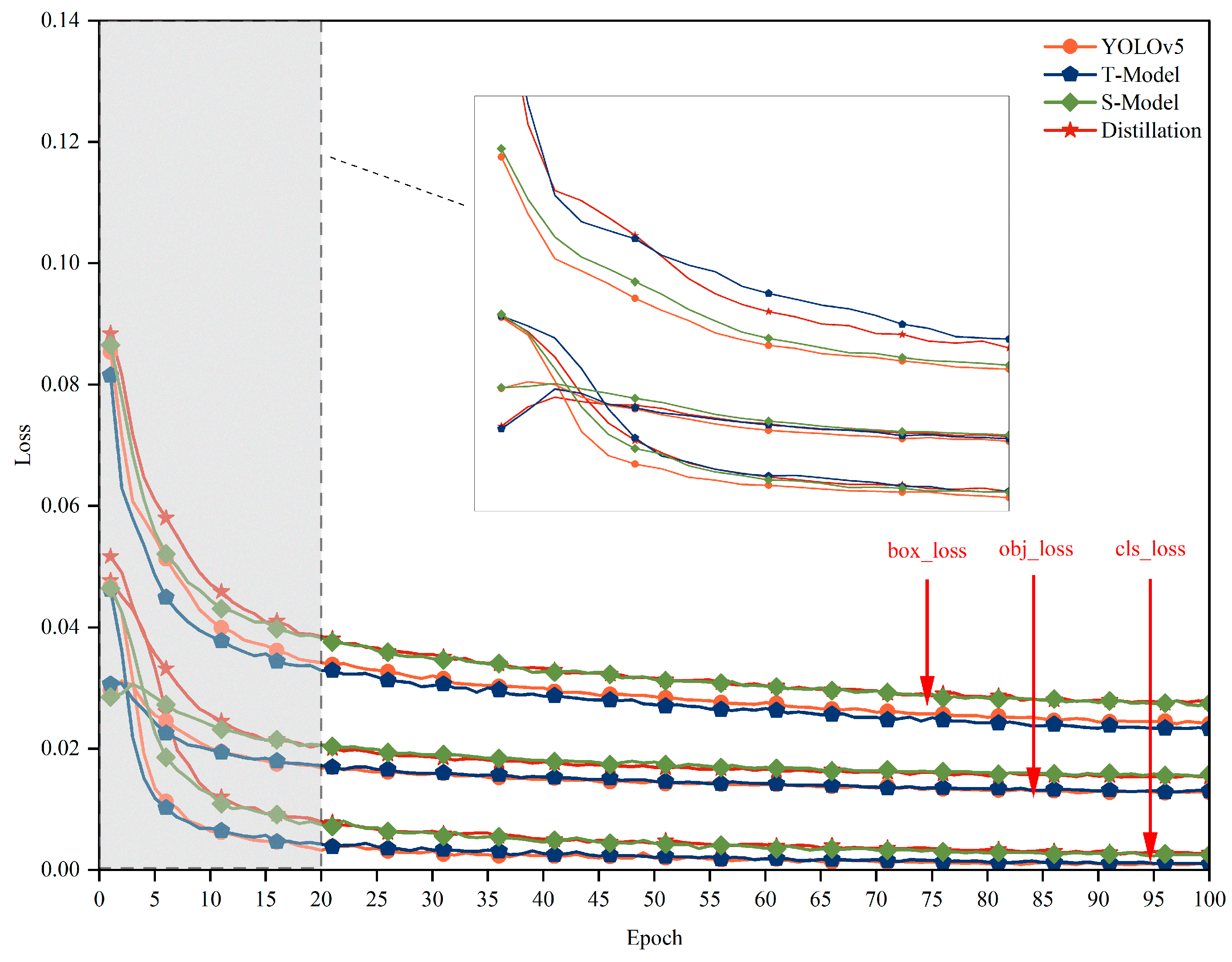
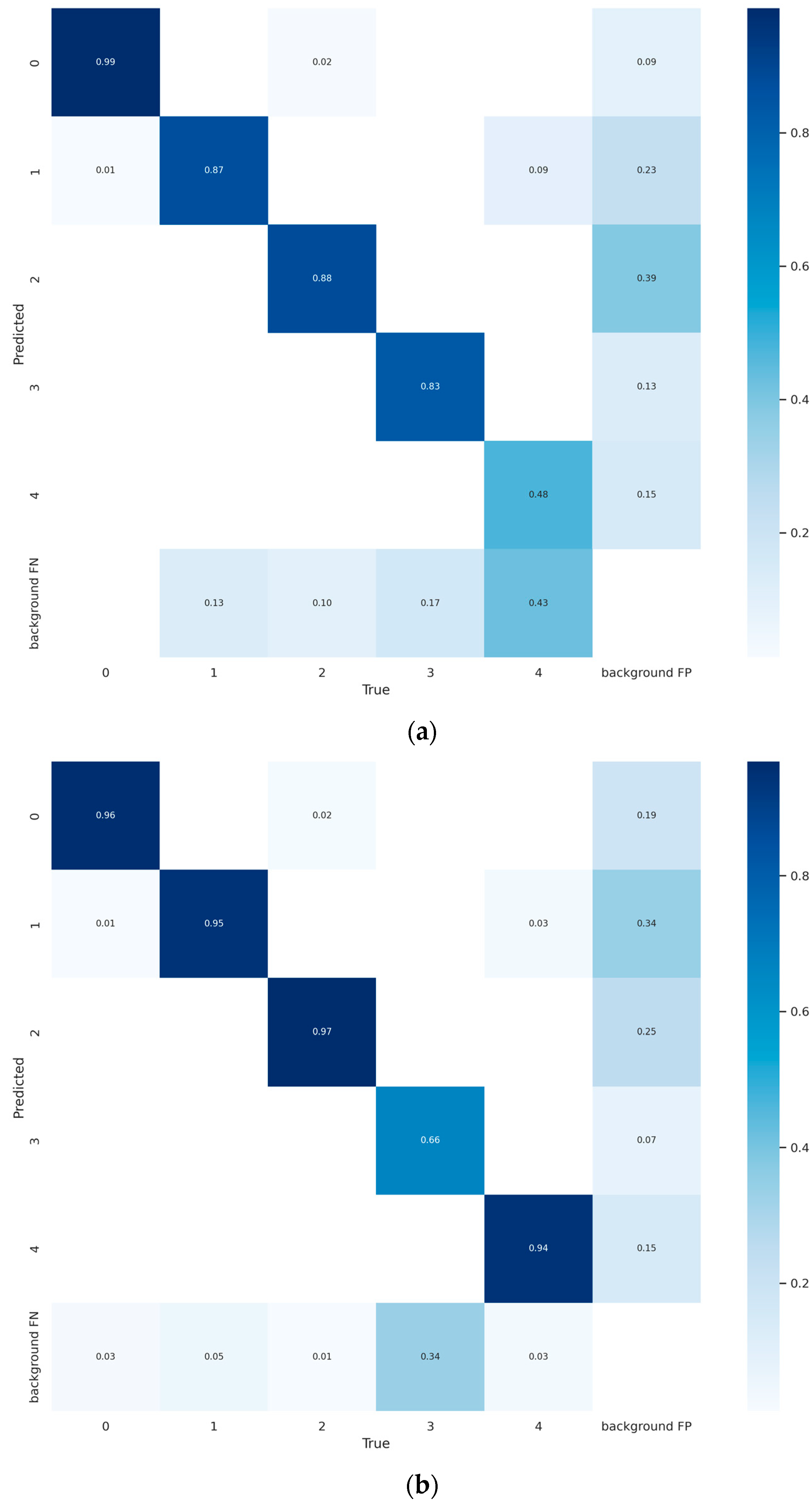
5. Experimental Results
6. Conclusions
Author Contributions
Funding
Data Availability Statement
Conflicts of Interest
References
- Minardo, A.; Catalano, E.; Coscetta, A.; Zeni, G.; Zhang, L.; Di Maio, C.; Vassallo, R.; Coviello, R.; Macchia, G.; Picarelli, L. Distributed fiber optic sensors for the monitoring of a tunnel crossing a landslide. Remote Sens. 2018, 10, 1291. [Google Scholar] [CrossRef] [Green Version]
- Monsberger, C.M.; Lienhart, W. Distributed fiber optic shape sensing of concrete structures. Sensors 2021, 21, 6098. [Google Scholar] [CrossRef] [PubMed]
- Afshani, A.; Kawakami, K.; Konishi, S.; Akagi, H. Study of infrared thermal application for detecting defects within tunnel lining. Tunn. Undergr. Space Technol. 2019, 86, 186–197. [Google Scholar] [CrossRef]
- Dong, Y.; Wang, J.; Wang, Z.; Zhang, X.; Gao, Y.; Sui, Q.; Jiang, P. A deep-learning-based multiple defect detection method for tunnel lining damages. IEEE Access 2019, 7, 182643–182657. [Google Scholar] [CrossRef]
- Xue, Y.; Li, Y. A fast detection method via region-based fully convolutional neural networks for shield tunnel lining defects. Comput.-Aided Civ. Infrastruct. Eng. 2018, 33, 638–654. [Google Scholar] [CrossRef]
- Zhou, Z.; Zhang, J.; Gong, C. Automatic detection method of tunnel lining multi-defects via an enhanced You Only Look Once network. Comput.-Aided Civ. Infrastruct. Eng. 2022, 37, 762–780. [Google Scholar] [CrossRef]
- Liu, Z.; Wu, W.; Gu, X.; Li, S.; Wang, L.; Zhang, T. Application of combining YOLO models and 3D GPR images in road detection and maintenance. Remote Sens. 2021, 13, 1081. [Google Scholar] [CrossRef]
- Zhu, A.; Chen, S.; Lu, F.; Ma, C.; Zhang, F. Recognition Method of Tunnel Lining Defects Based on Deep Learning. Wirel. Commun. Mob. Comput. 2021, 2021, 9070182. [Google Scholar] [CrossRef]
- Zhu, A.; Ma, C.; Chen, S.; Wang, B.; Guo, H. Tunnel Lining Defect Identification Method Based on Small Sample Learning. Wirel. Commun. Mob. Comput. 2022, 2022, 1096467. [Google Scholar] [CrossRef]
- Liu, M.; Liu, C.; Chen, Y.; Yan, Z.; Zhao, N. Radio frequency fingerprint collaborative intelligent blind identification for green radios. IEEE Trans. Green Commun. Netw. 2022, 7, 940–949. [Google Scholar] [CrossRef]
- Liu, M.; Zhang, Z.; Chen, Y.; Ge, J.; Zhao, N. Adversarial attack and defense on deep learning for air transportation communication jamming. IEEE Trans. Intell. Transp. Syst. 2023, 1–14. [Google Scholar] [CrossRef]
- Huang, Q. Weight-quantized squeezenet for resource-constrained robot vacuums for indoor obstacle classification. AI 2022, 3, 180–193. [Google Scholar] [CrossRef]
- Hu, W.; Che, Z.; Liu, N.; Li, M.; Tang, J.; Zhang, C.; Wang, J. Channel Pruning via Class-Aware Trace Ratio Optimization. IEEE Trans. Neural Netw. Learn. Syst. 2023, 1–13. [Google Scholar] [CrossRef]
- Zhang, S.; Qiang, B.; Yang, X.; Wei, X.; Chen, R.; Chen, L. Human Pose Estimation via an Ultra-Lightweight Pose Distillation Network. Electronics 2023, 12, 2593. [Google Scholar] [CrossRef]
- Zhao, Z.; Su, S.; Wei, J.; Tong, X.; Gao, W. Lightweight Infrared and Visible Image Fusion via Adaptive DenseNet with Knowledge Distillation. Electronics 2023, 12, 2773. [Google Scholar] [CrossRef]
- Hinton, G.; Vinyals, O.; Dean, J. Distilling the knowledge in a neural network. arXiv 2015, arXiv:1503.02531. [Google Scholar]
- Romero, A.; Ballas, N.; Kahou, S.E.; Chassang, A.; Gatta, C.; Bengio, Y. Fitnets: Hints for thin deep nets. arXiv 2014, arXiv:1412.6550. [Google Scholar]
- Zagoruyko, S.; Komodakis, N. Paying more attention to attention: Improving the performance of convolutional neural networks via attention transfer. arXiv 2016, arXiv:1612.03928. [Google Scholar]
- Redmon, J.; Divvala, S.; Girshick, R.; Farhadi, A. You only look once: Unified, real-time object detection. In Proceedings of the IEEE Conference on Computer Vision and Pattern Recognition, Las Vegas, NV, USA, 26 June–1 July 2016; pp. 779–788. [Google Scholar]
- Zhang, J.; Chen, H.; Yan, X.; Zhou, K.; Zhang, J.; Zhang, Y.; Jiang, H.; Shao, B. An Improved YOLOv5 Underwater Detector Based on an Attention Mechanism and Multi-Branch Reparameterization Module. Electronics 2023, 12, 2597. [Google Scholar] [CrossRef]
- de Moraes, J.L.; de Oliveira Neto, J.; Badue, C.; Oliveira-Santos, T.; de Souza, A.F. Yolo-Papaya: A Papaya Fruit Disease Detector and Classifier Using CNNs and Convolutional Block Attention Modules. Electronics 2023, 12, 2202. [Google Scholar] [CrossRef]
- Liu, Y.; Chu, H.; Song, L.; Zhang, Z.; Wei, X.; Chen, M.; Shen, J. An improved tuna-YOLO model based on YOLO v3 for real-time tuna detection considering lightweight deployment. J. Mar. Sci. Eng. 2023, 11, 542. [Google Scholar] [CrossRef]
- Xiao, P.; Xu, T.; Xiao, X.; Li, W.; Wang, H. Distillation Sparsity Training Algorithm for Accelerating Convolutional Neural Networks in Embedded Systems. Remote Sens. 2023, 15, 2609. [Google Scholar] [CrossRef]
- Hou, S.; Tuerhong, G.; Wushouer, M. UsbVisdaNet: User Behavior Visual Distillation and Attention Network for Multimodal Sentiment Classification. Sensors 2023, 23, 4829. [Google Scholar] [CrossRef]
- Wang, L.; Zhang, Y.; Xu, Y.; Yuan, R.; Li, S. Residual Depth Feature-Extraction Network for Infrared Small-Target Detection. Electronics 2023, 12, 2568. [Google Scholar] [CrossRef]
- He, K.; Zhang, X.; Ren, S.; Sun, J. Deep residual learning for image recognition. In Proceedings of the IEEE Conference on Computer Vision and Pattern Recognition, Las Vegas, NV, USA, 26 June–1 July 2016; pp. 770–778. [Google Scholar]
- Wu, X.; Shi, H.; Zhu, H. Fault Diagnosis for Rolling Bearings Based on Multiscale Feature Fusion Deep Residual Networks. Electronics 2023, 12, 768. [Google Scholar] [CrossRef]
- Muhammad, W.; Bhutto, Z.; Ansari, A.; Memon, M.L.; Kumar, R.; Hussain, A.; Shah, S.A.R.; Thaheem, I.; Ali, S. Multi-path deep CNN with residual inception network for single image super-resolution. Electronics 2021, 10, 1979. [Google Scholar] [CrossRef]


| Defect Type | Training Set | Validation Set | Test Set | Tags |
|---|---|---|---|---|
| BM | 1301 | 114 | 76 | 0 |
| TK | 1815 | 127 | 139 | 1 |
| KD | 904 | 78 | 254 | 2 |
| CS | 1136 | 80 | 197 | 3 |
| YBM | 1175 | 111 | 107 | 4 |
| Name | Configure |
|---|---|
| Equipment Model | TGRI-GPR200 |
| Center Frequency | 200 MHz |
| Operating Bandwidth | 100 MHz–500 MHz |
| Depth of detection | 10 m |
| Dynamic Range | 40 dB |
| Name | Configure |
|---|---|
| Operating System | Linux |
| Video Card | NVIDIA RTX3090 |
| Video Memory | 24G |
| Processor | Intel(R) Core i3-8100 |
| Programming Language | Python |
| Deep training framework | PyTorch |
| Programming Platforms | Pycharm |
| Name | Value |
|---|---|
| Pixel | 640 × 640 |
| Epoch | 100 |
| Batch size | 32 |
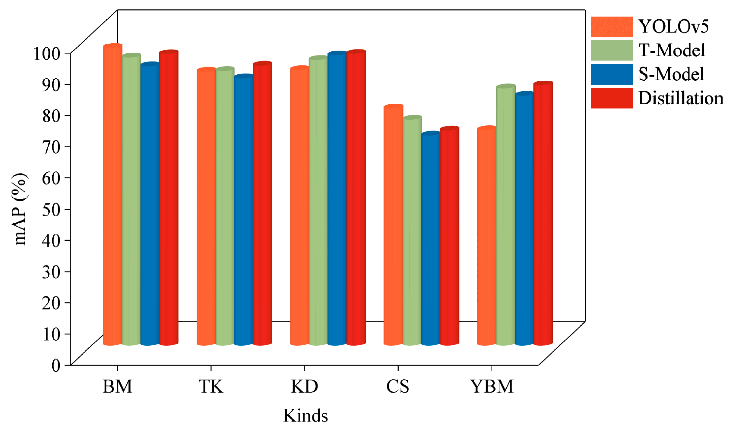
| Type | Average Accuracy Rate/% | ||||
|---|---|---|---|---|---|
| Models | BM | TK | KD | CS | YBM |
| Yolov5 | 95.6 | 87.9 | 88.4 | 76.1 | 69.1 |
| T-Model | 92.4 | 88.1 | 91.6 | 72.4 | 82.5 |
| S-Model | 89.6 | 85.8 | 93.1 | 67.4 | 80.2 |
| Distillation | 93.5 | 89.8 | 93.6 | 69.0 | 83.5 |
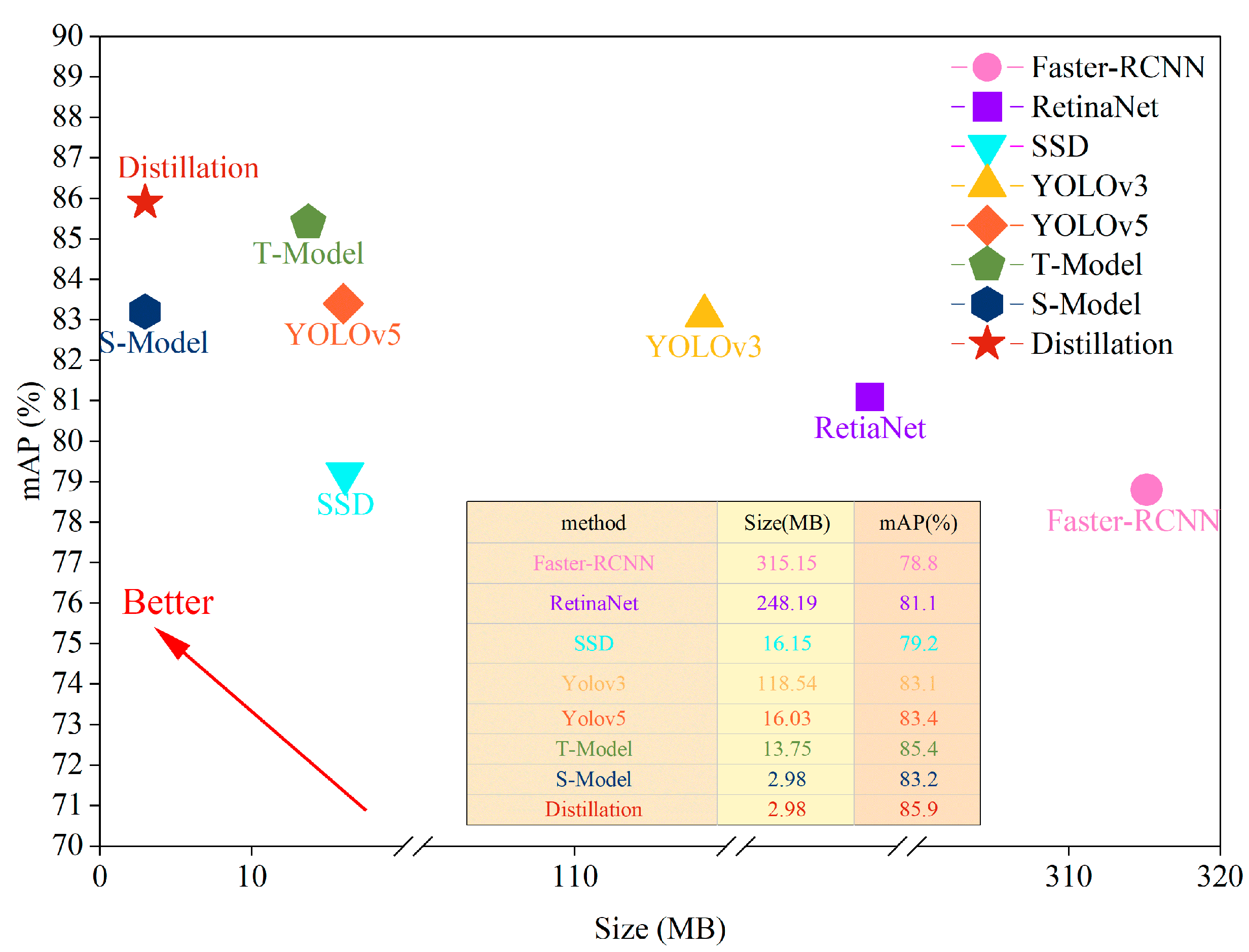
| Model | mAP@0.5 (%) | mAP@0.5:0.95 (%) | Precision (%) | Recall (%) | GFLOPS (G) | Size (MB) |
|---|---|---|---|---|---|---|
| Faster-RCNN | 78.8 | 48.8 | 78.6 | 80.2 | 88.2 | 315.15 |
| RetinaNet | 81.1 | 49.8 | 79.7 | 81.3 | 70.3 | 248.19 |
| SSD | 79.2 | 47.0 | 75.2 | 82.1 | 15.2 | 16.15 |
| Yolov3 | 83.1 | 49.1 | 80.3 | 81.6 | 154.6 | 118.54 |
| Yolov5 | 83.4 | 47.9 | 75.4 | 82.4 | 16.8 | 16.03 |
| T-Model | 85.4 | 49.6 | 76.3 | 80.3 | 15.8 | 13.75 |
| S-Model | 83.2 | 46.7 | 74.8 | 80.9 | 2.3 | 2.98 |
| Distillation | 85.9 | 50.3 | 77.4 | 83.1 | 2.3 | 2.98 |
Disclaimer/Publisher’s Note: The statements, opinions and data contained in all publications are solely those of the individual author(s) and contributor(s) and not of MDPI and/or the editor(s). MDPI and/or the editor(s) disclaim responsibility for any injury to people or property resulting from any ideas, methods, instructions or products referred to in the content. |
© 2023 by the authors. Licensee MDPI, Basel, Switzerland. This article is an open access article distributed under the terms and conditions of the Creative Commons Attribution (CC BY) license (https://creativecommons.org/licenses/by/4.0/).
Share and Cite
Zhu, A.; Wang, B.; Xie, J.; Ma, C. Lightweight Tunnel Defect Detection Algorithm Based on Knowledge Distillation. Electronics 2023, 12, 3222. https://doi.org/10.3390/electronics12153222
Zhu A, Wang B, Xie J, Ma C. Lightweight Tunnel Defect Detection Algorithm Based on Knowledge Distillation. Electronics. 2023; 12(15):3222. https://doi.org/10.3390/electronics12153222
Chicago/Turabian StyleZhu, Anfu, Bin Wang, Jiaxiao Xie, and Congxiao Ma. 2023. "Lightweight Tunnel Defect Detection Algorithm Based on Knowledge Distillation" Electronics 12, no. 15: 3222. https://doi.org/10.3390/electronics12153222