
Multi-Time Interval Dynamic Optimization Model of New Energy Output Based on Multi-Energy Storage Coordination
Abstract
:1. Introduction
- (1)
- To realize the dynamic optimization of new energy output, the optimal solution of new energy output is discretized to form a continuous function in time.
- (2)
- A dynamic optimization strategy is designed, which regards the multi-energy energy storage device and the new energy unit as a whole. By controlling the state of charge of the energy storage device, the output fluctuation of the new energy is suppressed.
- (3)
- Considering the adjustment cost of multiple types of regulating equipment connected to multi-energy power systems, the objective function of new energy output optimization of multi-energy power systems is established, and the model is solved based on distributed graph theory.
2. Multi-Energy Storage Model
2.1. Electrothermal Energy Storage Model
2.2. Battery Characteristic Model
2.3. Electro-Hydrogen Energy Storage Characteristic Model
3. Dynamic Optimization Strategy of New Energy Output Based on Multi-Energy Storage Control
3.1. Discretization Optimization of New Energy Output
3.2. Dynamic Optimization Strategy for New Energy Output
3.2.1. New Energy Unit Output Matrix Considering Multi-Energy Storage Control and Uncertainty Disturbance
3.2.2. Dynamic Optimization of New Energy Output Combination Matrix
4. Optimization Model for New Energy Output from Multi-Energy Grids
4.1. Objective Function
4.2. Constraints
4.2.1. Multi-Energy Power System New Energy Output Regulation Range Trade-Off Constraint
4.2.2. Constraints on the Regulation Characteristics of Thermal and Hydropower Units
4.2.3. Multi-Energy Storage Regulation Characteristics Constraints
4.2.4. Multi-Energy Regulation Balance Constraints
4.2.5. Multi-Energy Power System Network Constraints
4.3. Solving Algorithm
5. Example Analysis
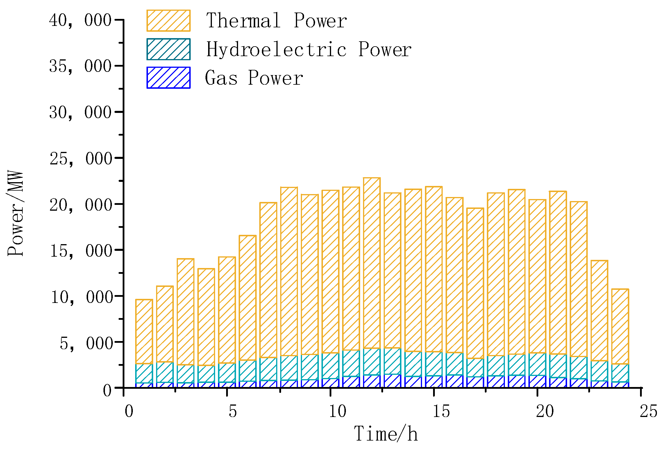
5.1. The Influence of Energy Storage Configuration on the Optimization Results
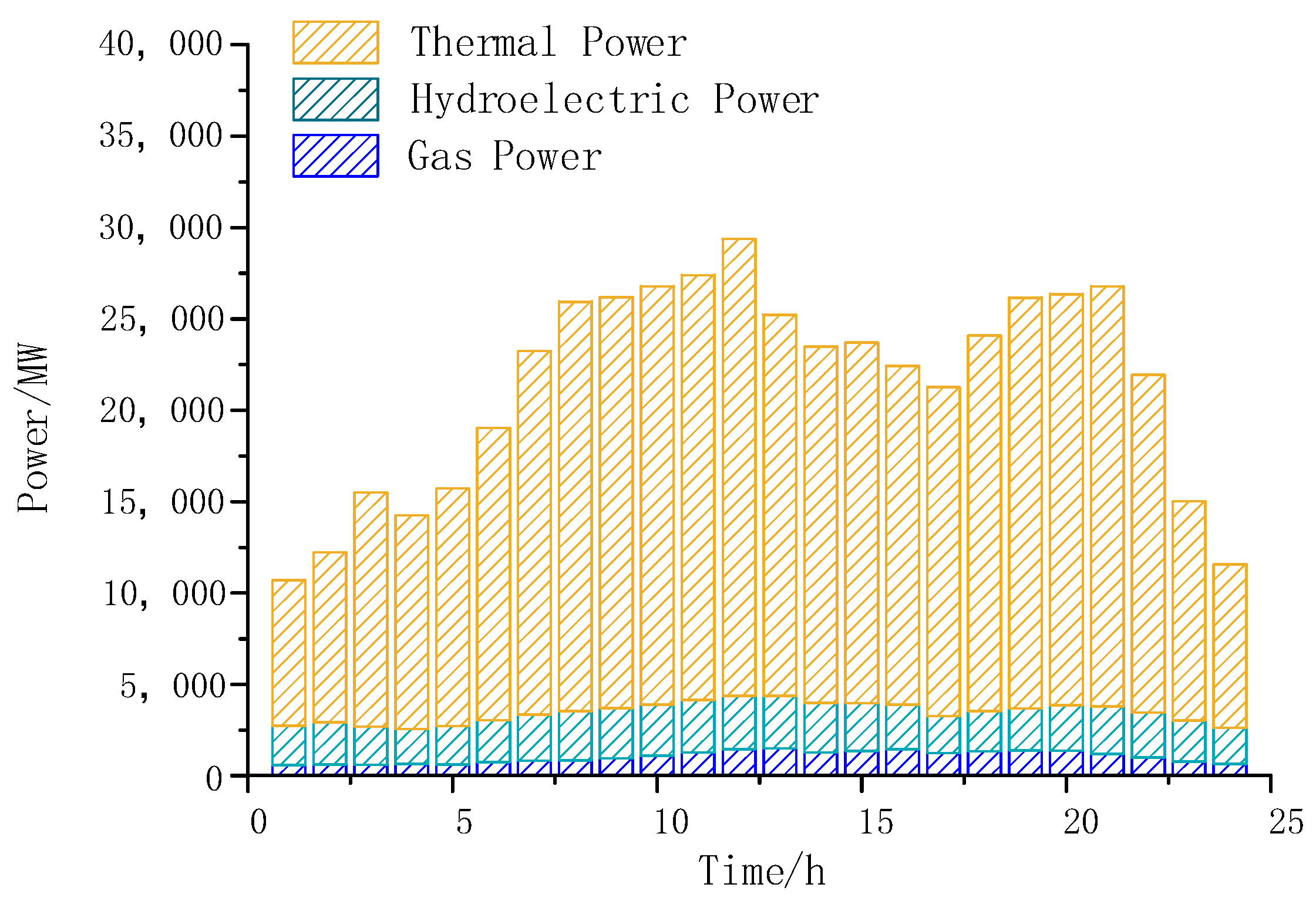
5.2. The Influence of New Energy Output Uncertainty on the Optimization Results
5.3. Comparison of Optimization Results under Another Solving Algorithm
6. Conclusions and Prospects
- (1)
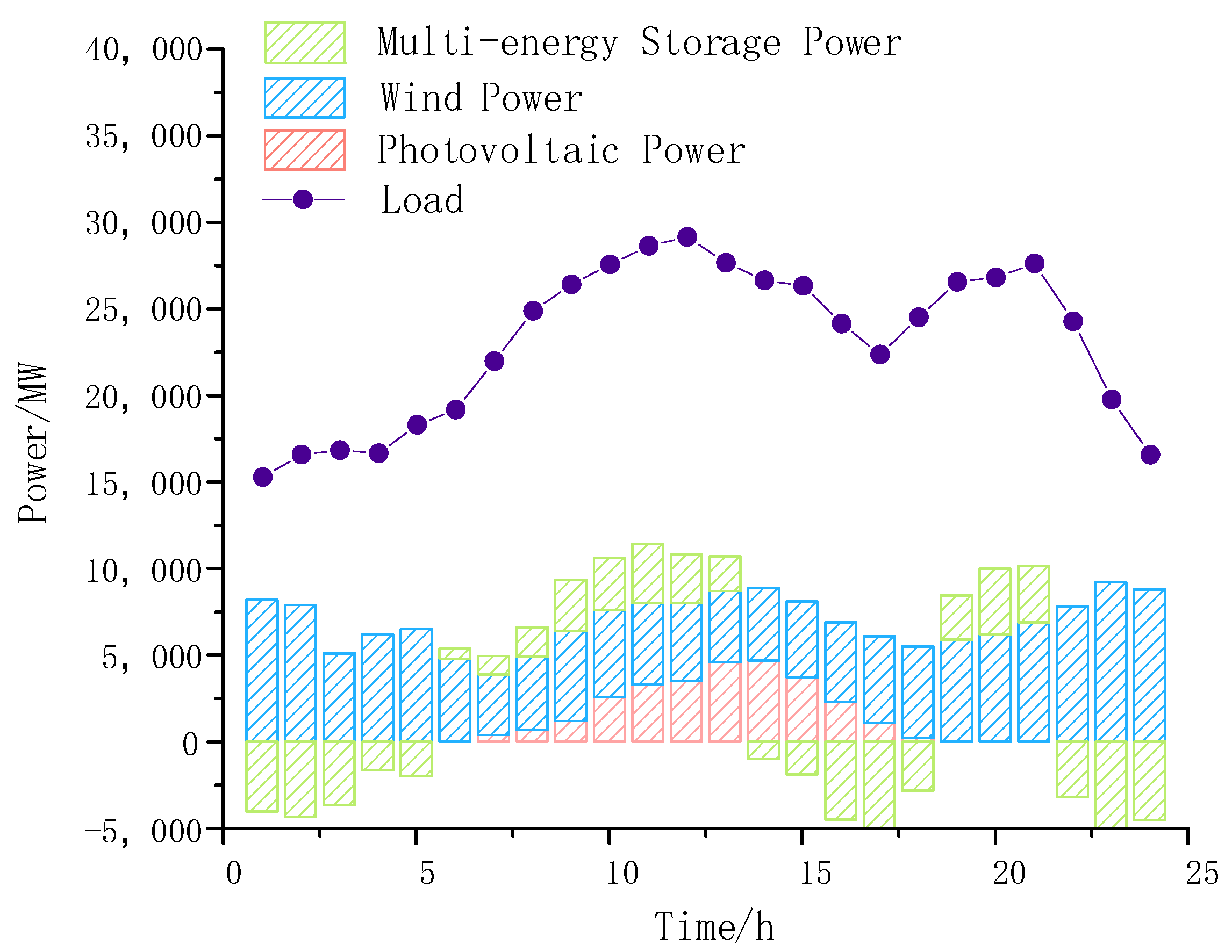
- In the process of optimizing new energy output based on multi-energy storage devices, each energy storage device participates in regulation, which can fully unleash the charging and discharging potential of the energy storage device and effectively suppress fluctuations in new energy output.
- (2)
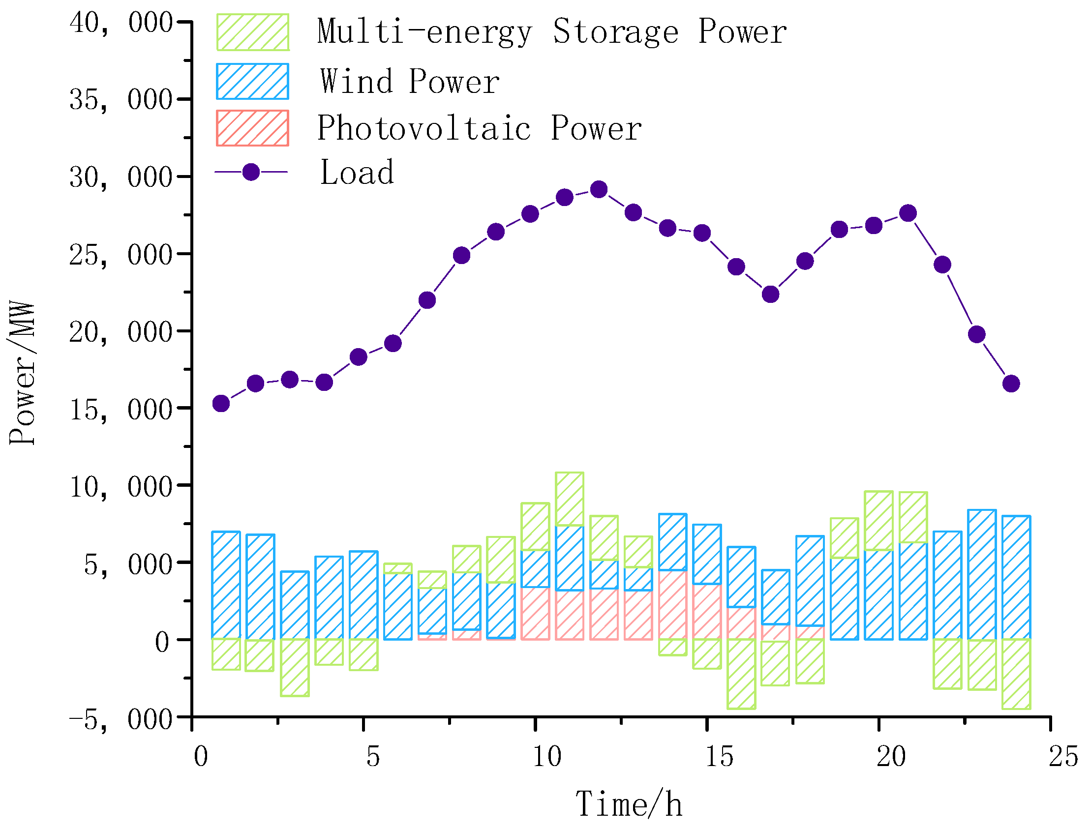
- The enhancement of uncertainty in the output of new energy will inevitably lead to an increase in the system’s peak-shaving pressure and cost. However, using the dynamic optimization algorithm proposed in this article allows multi-energy systems to still provide sufficient load reserve and temporary stable reserve even when traditional power generation units use smaller start-up methods, reducing the system’s peak-shaving pressure.
- (3)
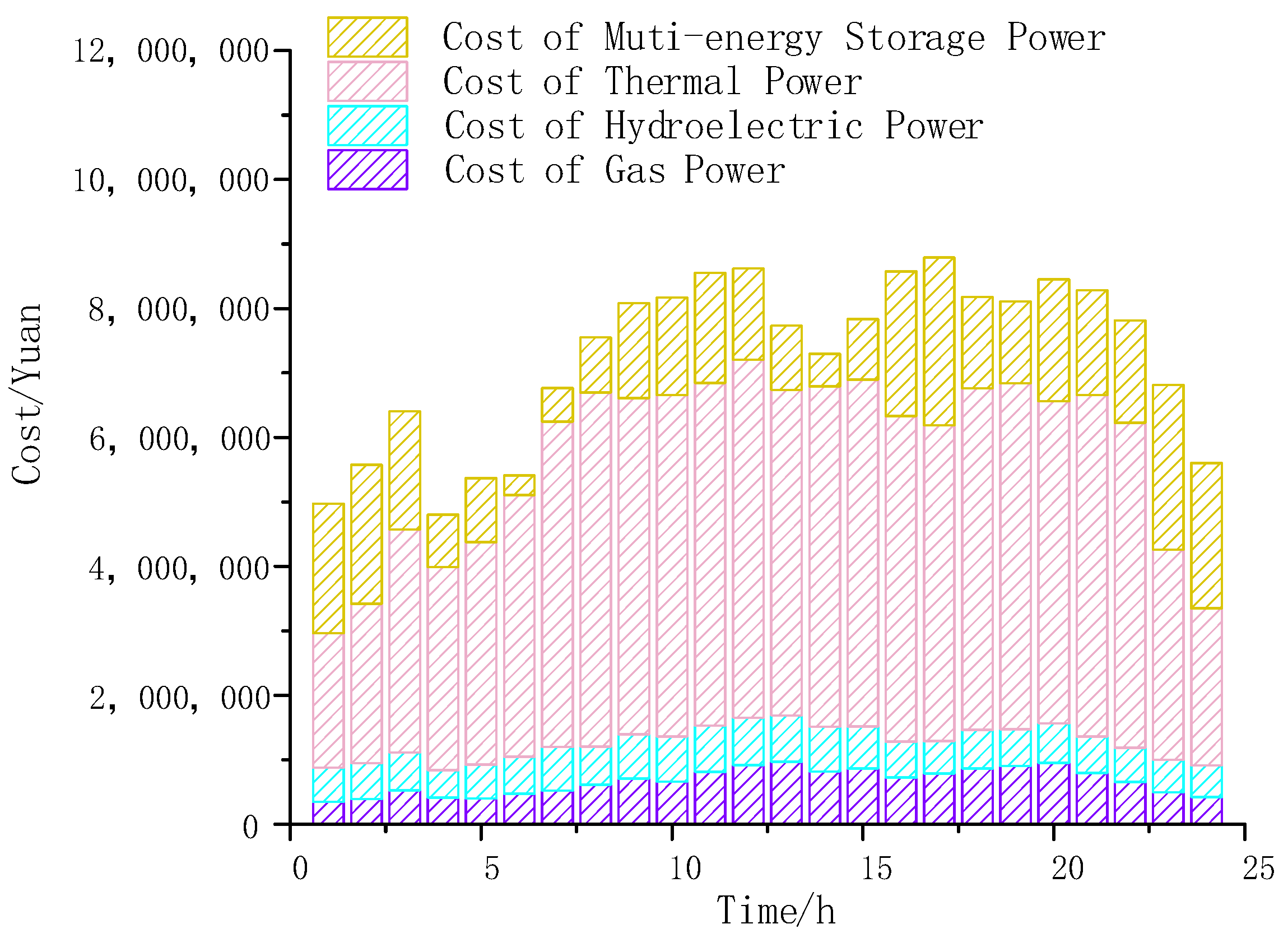
- In terms of peak-shaving costs, the method proposed in this article can suppress the uncertainty of new energy output at a lower cost and improve the operational economy of multi-energy systems.
Author Contributions
Funding
Data Availability Statement
Conflicts of Interest
References
- Li, Y.; Zhang, H.; Liang, X.; Huang, B. Event-triggered based distributed cooperative energy management for multi-energy systems. IEEE Trans. Ind. Inf. 2019, 15, 2008–2022. [Google Scholar] [CrossRef]
- Luo, S.; Peng, K.; Hu, C.; Ma, R. Consensus-Based Distributed Optimal Dispatch of Integrated Energy Microgrid. Electronics 2023, 12, 1468. [Google Scholar] [CrossRef]
- Gao, F.; Gao, J.; Huang, N.; Wu, H. Optimal Configuration and Scheduling Model of a Multi-Park Integrated Energy System Based on Sustainable Development. Electronics 2023, 12, 1204. [Google Scholar] [CrossRef]
- Zhang, J.; Li, H.; Li, W.; Zhang, H.; Wang, B. Discussion on the pathways of China’s electrification polices to pursue the carbon neutralization target. Electr. Power Constr. 2022, 43, 47–53. [Google Scholar]
- Li, Y.; Gao, D.W.; Gao, W.; Zhang, H.; Zhou, J. Double-Mode Energy Management for Multi-Energy System via Distributed Dynamic Event-Triggered Newton-Raphson Algorithm. IEEE Trans. Smart Grid 2020, 11, 5339–5356. [Google Scholar] [CrossRef]
- Li, Y.; Gao, D.W.; Gao, W.; Zhang, H.; Zhou, J. A Distributed Double-Newton Descent Algorithm for Cooperative Energy Management of Multiple Energy Bodies in Energy Internet. IEEE Trans. Ind. Inf. 2021, 17, 5993–6003. [Google Scholar] [CrossRef]
- Jin, H.; Teng, Y.; Zhang, T.; Wang, Z.; Deng, B. A locational Marginal Price-Based Partition Optimal Economic Dispatch Model of Multi-Energy Systems. Front. Energy Res. 2021, 9, 694983. [Google Scholar] [CrossRef]
- Hu, H.; Sun, X.; Zeng, B.; Gong, D.; Zhang, Y. Enhanced evolutionary multi-objective optimization-based dispatch of coal mine integrated energy system with flexible load. Appl. Energy 2022, 307, 118130. [Google Scholar] [CrossRef]
- Lei, Y.; Chen, X.; Jiang, K.; Li, H.; Zou, Z. A Novel Methodology for Electric-Thermal Mixed Power Flow Simulation and Transmission Loss Analysis in Multi-Energy Micro-Grids. Front. Energy Res. 2021, 8, 620259. [Google Scholar] [CrossRef]
- Wei, J.; Zhang, Y.; Wang, J.; Cao, X.; Khan, M.A. Multi-period planning of multi-energy microgrid with multi-type uncertainties using chance constrained information gap decision method. Appl. Energy 2020, 260, 114188. [Google Scholar] [CrossRef]
- Jiang, Y.; Wan, C.; Chen, C.; Shahidehpour, M.; Song, Y. A Hybrid Stochastic-Interval Operation Strategy for Multi-Energy Microgrids. IEEE Trans. Smart Grid 2019, 11, 440–456. [Google Scholar] [CrossRef]
- Wang, R.; Sun, Q.; Hu, W.; Li, Y.; Ma, D.; Wang, P. SoC-Based Droop Coefficients Stability Region Analysis of the Battery for Stand-Alone Supply Systems with Constant Power Loads. IEEE Trans. Power Electron. 2021, 36, 7866–7879. [Google Scholar] [CrossRef]
- Si, F.; Han, Y.; Zhao, Q.; Wang, J. Cost-effective operation of the urban energy system with variable supply and demand via coordination of multi-energy flows. Energy 2020, 203, 117827. [Google Scholar] [CrossRef]
- Azimi, M.; Salami, A. A new approach on quantification of flexibility index in multi-carrier energy systems towards optimally energy hub management. Energy 2021, 232, 120973. [Google Scholar] [CrossRef]
- Sun, P.; Teng, Y.; Chen, Z. Robust coordinated optimization for multi-energy systems based on multiple thermal inertia numerical simulation and uncertainty analysis. Appl. Energy 2021, 296, 116982. [Google Scholar] [CrossRef]
- Feng, L.; Jian, Q.; Tian, H.; Zhao, L.; Liu, R.; Zhao, E. Optimal dispatch and economic evaluation of zero carbon park considering capacity attenuation of shared energy storage. Electr. Power Constr. 2022, 43, 112–121. [Google Scholar]
- Yan, J.; Teng, Y.; Chen, Z. Optimization of Multi-energy Microgrids with Waste Process Capacity for Electricity-hydrogen Charging Services. CSEE J. Power Energy Syst. 2021, 8, 380–391. [Google Scholar]
- Weng, C.; Hu, Z.; Zhang, C.; Li, X.; Wang, F. Distributed planning model of renewable vehicle energy supply station considering seasonal hydrogen storage. Electr. Power Constr. 2022, 43, 37–46. [Google Scholar]
- Shi, Y.; Jin, L.; Li, S.; Li, J.; Qiang, J.; Gerontitis, D.K. Novel Discrete-Time Recurrent Neural Networks Handling Discrete-Form Time-Variant Multi-Augmented Sylvester Matrix Problems and Manipulator Application. IEEE Trans. Neural Netw. Learn. Syst. 2022, 33, 587–599. [Google Scholar] [CrossRef]
- Mei, J.; Ren, W.; Chen, J. Distributed Consensus of Second-Order Multi-Agent Systems with Heterogeneous Unknown Inertias and Control Gains Under a Directed Graph. IEEE Trans. Autom. Control 2015, 61, 2019–2034. [Google Scholar] [CrossRef]
- Teng, Y.; Sun, P.; Luo, H.; Chen, Z. Autonomous Optimization Operation Model for Multi-source Microgrid Considering Electrothermal Hybrid Energy Storage. Proc. CSEE 2019, 39, 5316–5324+5578. [Google Scholar]


| Node Number | Power Source Type | Capacity (MW) |
|---|---|---|
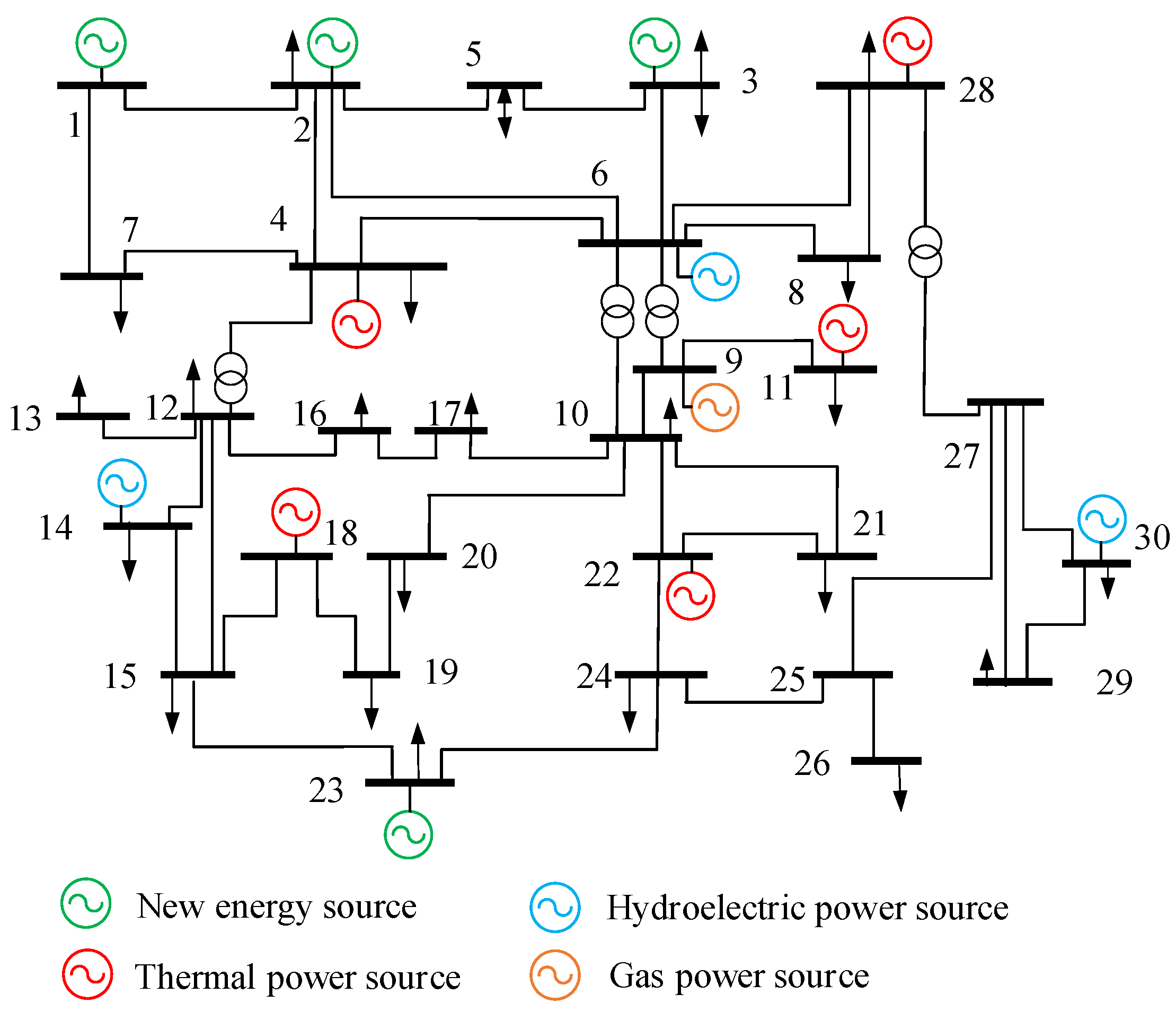
| 1, 3, 23 | Wind power | 11,000 |
| 2 | Photovoltaic power | 4800 |
| 4, 11, 18, 22, 28 | Thermal power | 36,500 |
| 14, 6, 30 | Hydroelectric power | 3000 |
| 9 | Gas power | 1500 |
| Node Number | Power Source Type | Capacity (MWh) |
|---|---|---|
| 8, 9 | Electric heating and heat storage equipment | 11,000 |
| 5 | Electric hydrogen production, hydrogen storage equipment, and hydrogen cell | 4800 |
| 7, 24 | Chemical battery | 1500 |
| Simulation Scenario | Whether the Energy Storage Device Is Involved in Regulation | New Energy Output Uncertainty | Algorithm |
|---|---|---|---|
| S1 | NO | 5% | Proposed algorithm |
| S2 | YES | 5% | Proposed algorithm |
| S3 | YES | 20% | Proposed algorithm |
| S4 | YES | 20% | Multi-objective differential algorithm |
Disclaimer/Publisher’s Note: The statements, opinions and data contained in all publications are solely those of the individual author(s) and contributor(s) and not of MDPI and/or the editor(s). MDPI and/or the editor(s) disclaim responsibility for any injury to people or property resulting from any ideas, methods, instructions or products referred to in the content. |
© 2023 by the authors. Licensee MDPI, Basel, Switzerland. This article is an open access article distributed under the terms and conditions of the Creative Commons Attribution (CC BY) license (https://creativecommons.org/licenses/by/4.0/).
Share and Cite
Wang, Q.; Cheng, S.; Ma, S.; Chen, Z. Multi-Time Interval Dynamic Optimization Model of New Energy Output Based on Multi-Energy Storage Coordination. Electronics 2023, 12, 3056. https://doi.org/10.3390/electronics12143056
Wang Q, Cheng S, Ma S, Chen Z. Multi-Time Interval Dynamic Optimization Model of New Energy Output Based on Multi-Energy Storage Coordination. Electronics. 2023; 12(14):3056. https://doi.org/10.3390/electronics12143056
Chicago/Turabian StyleWang, Qiwei, Songqing Cheng, Shaohua Ma, and Zhe Chen. 2023. "Multi-Time Interval Dynamic Optimization Model of New Energy Output Based on Multi-Energy Storage Coordination" Electronics 12, no. 14: 3056. https://doi.org/10.3390/electronics12143056