Frequency Support Control of Multi-Terminal Direct Current System Integrated Offshore Wind Farms Considering Direct Current Side Stability

Abstract

The frequency stability of modern power systems is challenged due to widespread application of large-scale renewable energy systems, of which the offshore wind farm (OWF) is one of the dominant resources. The OWFs are usually integrated into the grid by multi-terminal direct current (MTDC) transmission systems, which makes the energy flow complicated and the frequency control design challenging. A frequency support control method of MTDC system integrated OWFs (referred to as the OWF-MTDC system) is proposed in this paper. First, the wind turbine generation system (WTGS) is controlled to reserve a certain amount of available power according to the real-time wind speed for more comprehensive frequency regulation. Then, the frequency support control of OWFs is designed, and they can release the rotor kinetic energy and reserved power to support the onshore grid frequency. In addition, the virtual inertia control of a modular multi-level converter (MMC) is designed, which can also provide frequency support in an emergency by use of the DC capacitor. To ensure that the frequency control of the OWF-MTDC system does not degrade the stability of the system, a detailed DC impedance model of the MMC-based MTDC systems is developed, considering the constant power control and DC voltage control. Based on the impedance model, the impact of the frequency control coefficients on the DC side stability of the MTDC system is analyzed. Simulation results validate the stability analysis and verify the proposed frequency control method, which can effectively provide frequency support to the onshore power grid.

1. Introduction

Offshore wind farms (OWFs) are developing rapidly and have attracted considerable attention in the field of renewable energy grid integration research due to their remarkable advantages, such as small footprint and high annual operating hours [1]. Due to the large scale of OWFs and the long distance between OWFs and onshore grids, voltage source converter-based multi-terminal direct current (VSC-MTDC) transmission technology is considered to be the most suitable option to integrate OWFs into the grid [2,3], making the OWF-MTDC system widely applied. The increasing penetration of wind power and other renewable energy sources significantly reduces the grid inertia, but the OWFs do not respond to grid frequency fluctuation under the conventional control scheme, which threatens the grid frequency stability [4]. To ensure safe and stable operation of the power system, research on frequency support control of OWF-MTDC systems is necessary and urgent.

The research on frequency control usually focuses on microgrids at first. For instance, the authors of [5] proposed a distributed event-triggered secondary control for frequency/voltage restoration and power sharing in cyber-physical microgrids. However, this approach may result in zero internal execution time, which leads to an accumulation of event times, also known as the Zeno phenomenon. In [6], the grid situational awareness system is analyzed, and the smart grid situational awareness model and conceptual design is presented, based on which the event-triggered strategy naturally excludes the Zeno phenomenon. As for the frequency control of OWFs for large-scale grid support, some attempts have been made to explore the assistance from the energy storage system (ESS) with its flexible charge–discharge capability [7], but the ESS will bring in nonnegligible cost. Moreover, the MTDC system in charge of integrating OWFs into the grid can provide frequency support as well. In [8], a frequency support strategy was developed for AC grids connected by an MTDC system, where the frequency of the disturbed grid can be restored by dispersing the disturbance to all interconnected grids. However, this may lead to severe frequency drops in other AC grids, and the frequency regulation capabilities of MMCs have not been fully utilized. Although the above control methods achieve a certain frequency support performance, they barely explore the potential frequency regulation capability of OWFs.

The wind turbine generation system (WTGS) typically operates in maximum power point tracking (MPPT) mode, and its output power is decoupled from the grid frequency. To realize grid frequency support, the WTGSs can emulate the inertia or frequency damping characteristics of synchronous generators. To emulate the inertia characteristic, the rate of change of frequency (RoCoF) signal can be transferred to the rotor side converter (RSC) of an OWF to release rotor kinetic energy and output required power when frequency events occur [9,10,11]. Notably, the rotor kinetic energy that the WTGS can release for frequency support is determined by the real-time wind speed and rotor speed [12]. A low wind speed corresponds to a low rotor speed, indicating less kinetic energy stored in the rotor. In this case, if the WTGS overexploits the kinetic energy of the rotor, it may trigger low-speed disconnection of the WTGS [13], which would result in serious consequences. On the other hand, the virtual inertia provided by the rotor kinetic energy mainly supports the grid during a short period after a fault, while the WTGS may even absorb power from the grid during the rotor speed recovery period, which will threaten the long-term frequency stability. To address this issue, power reserve control (PRC) can be employed to operate the WTGS away from the maximum power point, i.e., to reserve a certain amount of available output power to provide stable active power support when the frequency drops [14]. Considering the difference in operating wind speeds among different OWFs, the reserve power of WTGSs should be reasonably set according to the real-time maximum available power, and the additional power required for frequency regulation should also be manipulated fairly based on the operating status of each WTGS. A distributed framework is proposed in [15] to issue uniform torque and pitch angle instructions of wind turbines for equal distribution of power reserve requirements. Moreover, a dynamic power reserve strategy is proposed in [16] to coordinate OWFs under different wind speed zones and analyze the feasibility of rotor overspeed control to achieve variable virtual inertia. Although the discussed research can realize frequency support from OWFs, the coordination with MMCs in the MTDC system has not been discussed.

Notably, the DC capacitors in the MMCs of MTDC systems can also be utilized to provide virtual inertia, which is realized by releasing electrostatic energy from the capacitor in emergencies [17]. A simplified approach is to convert frequency changes into a DC voltage reference value through droop control, thereby controlling the charging and discharging of the DC capacitor [18,19]. However, the frequency–voltage droop control alters the control framework of the MMC, which may threaten the stability of the MTDC system or lead to resonance instability due to the coupling effect between the capacitive MMC and inductive DC lines [20]. In the literature, the droop coefficient is usually set directly according to the frequency deviation and voltage deviation thresholds, without considering the impact of the droop coefficient on system stability. Therefore, to avoid large-scale stability issues, it is necessary to analyze the resonance stability of the MTDC system when providing frequency support.

In order to analyze the resonance stability of the MTDC system, the models of MMCs should first be developed. Among the existing techniques, the impedance analysis method has a clear physical meaning and relatively simple calculation, so it is widely used in the resonance analysis of high-voltage direct current (HVDC) systems [21]. The internal dynamic characteristics of the MMC are complex, and its impedance model is difficult to derive. References [22,23] obtain an accurate impedance model of MMCs based on the harmonic state space and harmonic linearization method, but the order of the model is high, which is not conducive to the analysis of multi-terminal system stability. References [24,25,26] proposed several different DC side impedance models for the flexible DC transmission system based on the two-level voltage source converter, and these models were used for DC side resonance analysis. However, although the literature has achieved results on the modeling of MMCs and OWFs when participating in frequency regulation, the impact of frequency control coefficients of MMCs on the stability of MTDC systems has not been measured with a detailed analysis, and the design of the frequency control of OWFs and MTDC systems lacks supportive instruction.

To address the above issues, this paper proposes the frequency support control of OWF-MTDC systems considering the coordination of OWFs and MMCs in frequency regulation. Then, this paper develops the impedance model of the OWF-MTDC system with frequency support control, based on which the impact of frequency control coefficients on the stability of the MTDC system is analyzed. It further supports the design of frequency control coefficients in the OWF-MTDC system. The rest of the paper is organized as follows. The power reserve control and additional power control for WTGSs as well as the virtual inertia control of DC capacitors in MMCs are designed in Section 2. Then, the equivalent impedance model of MMCs and further the model of the MTDC system are developed in Section 3, based on which the impact of frequency control on the stability of the MTDC system is analyzed, providing the design basis for the frequency control coefficient of MMCs proposed in Section 2. Section 4 describes the case study in PSCAD/EMTDC software, which validates the performance of the control method and the stability analysis results. Section 5 concludes this paper.

2. Frequency Support Control of OWF-MTDC Systems

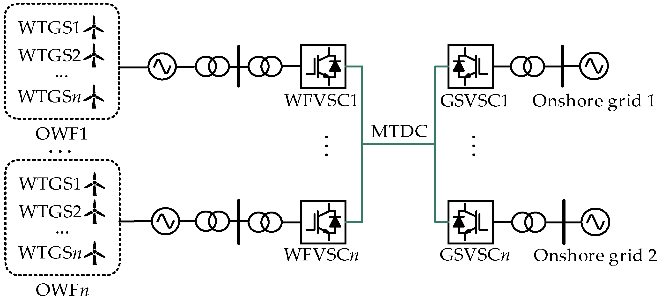
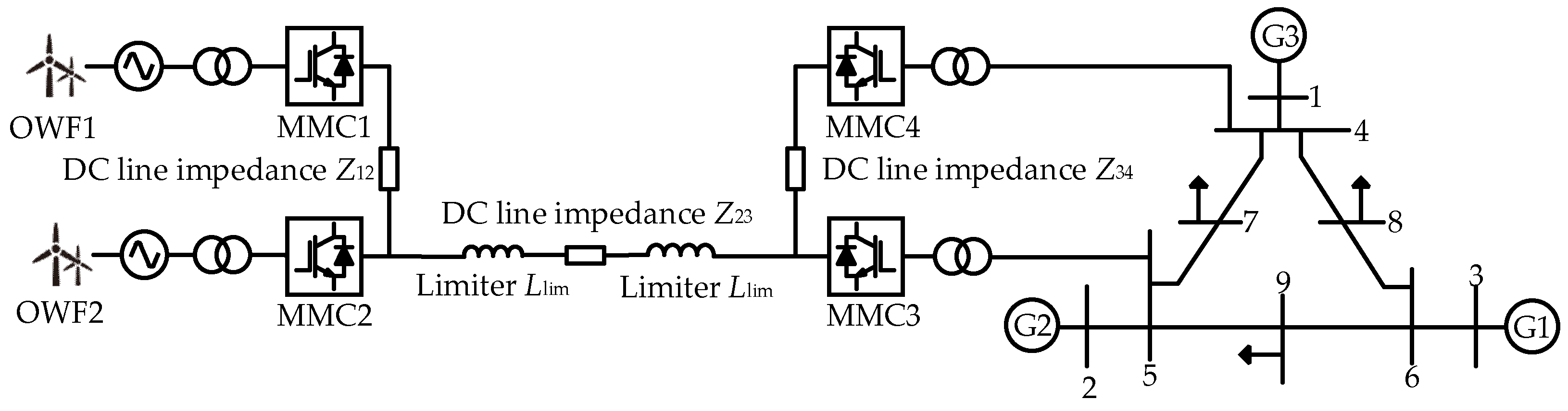
2.1. Configuration of OWF-MTDC System

The typical configuration of an OWF-MTDC system is radial topology [27], as shown in Figure 1. The power generated by the OWFs is transferred to the wind farm voltage source converter (WFVSC), then transferred to the grid side voltage source converter (GSVSC) via DC cables, and finally integrated into the onshore power grid. The WFVSC usually adopts island control to regulate the (OWF side) grid frequency and AC voltage, forming the AC grid of OWFs. The GSVSC usually adopts DC voltage control and active power control to maintain the DC voltage and manipulate power supply.

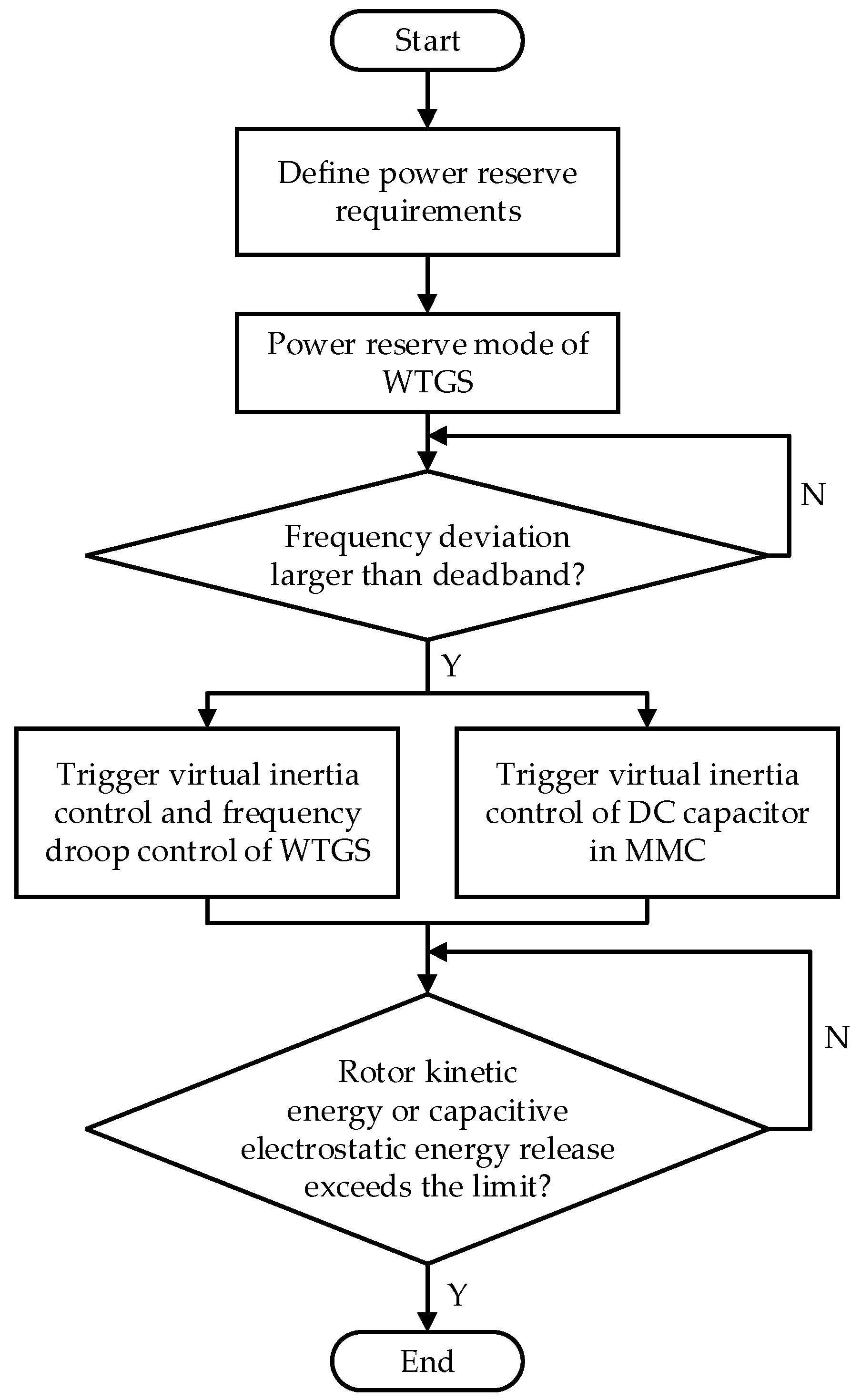
2.2. Power Reserve Control of WTGS

WTGSs usually operate in MPPT mode to output the maximum available power under real-time wind speed. The maximum available power of a WTGS is given by [28]

$$P_{\mathrm{opt}}=k_{\mathrm{opt}}{\omega }_{\mathrm{r}}^3$$

(1)

where P_opt is the maximum available output power of the WTGS, w_r is the rotor speed of the wind turbine, and k_opt is the power tracking curve coefficient of the WTGS when operating in MPPT mode, which is given by

$$k_{\mathrm{opt}}=\frac{\pi \rho R^5{C}_{\mathrm{p}}^{\max }}{2{\lambda }_{\mathrm{opt}}^3}$$

(2)

where ρ is the air density, R is the radius of the blade, $C_{\mathrm{p}}^{\max }$ is the maximum wind energy utilization coefficient, λ_opt is the optimal tip speed ratio.

In conventional control, the power reference obtained by the MPPT algorithm is transferred to the active power control of the RSC of WTGS. This allows the WTGS to adjust its rotor speed in time to capture the maximum available power, while the grid side converter (GSC) of the WTGS is responsible for maintaining DC voltage. Obviously, the WTGS operating in MPPT mode cannot supply excess power to the grid when the grid is experiencing power shortage, and the underfrequency event will then occur. Thus, for the WTGS to provide stable and continuous frequency support to the grid, it is necessary to reserve a certain amount of power in advance, i.e., to adopt PRC (also known as de-loading control). The PRC methods include overspeed control and pitch angle control. Both methods can cause the WTGS to deviate from its optimal operating point [29]. By setting a constant power reserve rate (d%) for all the WTGSs in an OWF, the WTGSs operating at high wind speeds will perform more power reserve and primary frequency regulation tasks. By inputting the power reference obtained from the reserved power curve into the RSC, the WTGS can operate at the power reserve point. The MPPT curve and d% reserved power curve of the WTGS at different wind speeds are shown in Figure 2, where v_a and v_b are the cut-in wind speed the rated wind speed of the WTGS.

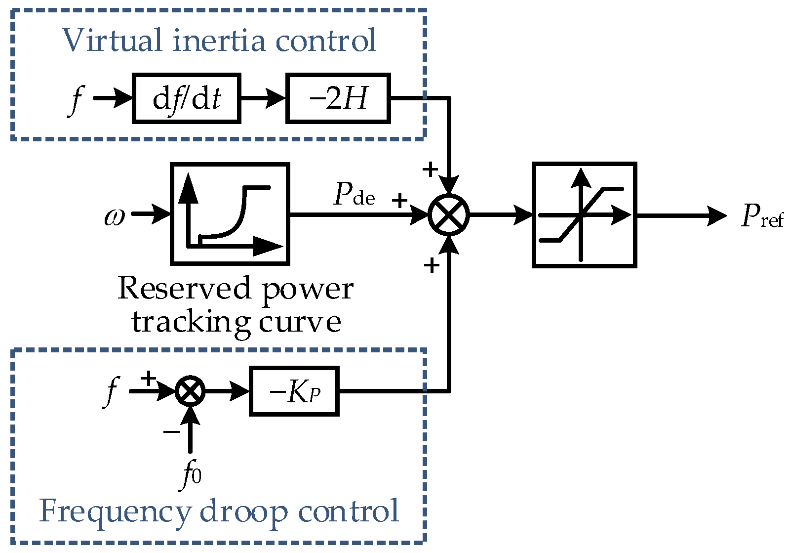
2.3. Frequency Support Control of WTGS

Since the rotor speed of the WTGS does not respond to the onshore grid frequency, it is necessary to introduce the frequency signal into the WTGS to artificially couple the rotor speed to the frequency. Considering that the grid frequency is mainly governed by the synchronous generator, the most effective frequency support method for the WTGS is to emulate inertia and frequency damping characteristics.

By introducing the RoCoF signal into the active power controller of the RSC as an additional droop loop, the rotor kinetic energy of the WTGS can be used to emulate the inertia response, which is called virtual inertia control. Alternatively, adding a frequency–power droop control to the active power controller of the RSC can emulate frequency damping characteristics for the WTGS. With the virtual inertia control and frequency droop control, the power reference of the RSC is given by

$$P_{\mathrm{ref}}=P_{\mathrm{de}}-2H\frac{\mathrm{d}f}{\mathrm{d}t}-K_{\mathrm{P}}\left(f-f_0\right)$$

(3)

where the second term represents the virtual inertia control and the third term represents the droop control.

Considering the variability of wind speed, the virtual inertia constant and frequency–power droop coefficient should be set according to the actual operating condition of the WTGS, which can be expressed as

$$H=\frac{{\omega }_0^2-{\omega }_{\min }^2}{{\omega }_{\max }^2-{\omega }_{\min }^2}\cdot H_0$$

(4)

where H is the virtual inertia constant for the WTGS, ω_max and ω_min are the maximum and minimum speed of the WTGS for normal operation, respectively, ω₀ is the rotor speed before disturbance, and H₀ is the initial virtual inertia.

$$K_{\mathrm{P}}=\frac{P_{\mathrm{res}}}{P_{\mathrm{rated}}}\cdot K_{\mathrm{P}0}$$

(5)

where K_P is the droop coefficient for the WTGS, P_res is the power reserve value, P_rated is the rated power of the WTGS, and K_P0 is the initial droop coefficient.

The active power control diagram of the RSC is shown in Figure 3, where P_ref is the power reference with virtual inertia control and droop control, P_de is the power reference obtained from the reserved power tracking curve, H is the virtual inertia, K_P is the frequency–power droop coefficient, f is the real-time frequency, f₀ is the rated frequency.

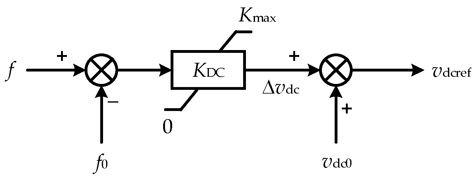
2.4. Virtual Inertia Control of DC Capacitor in MMC

The virtual inertia can also be provided by the DC capacitors in the MMC of MTDC system. By regulating the charging or discharging of the DC capacitor, the frequency–power characteristic of the synchronous generator rotor can be emulated, and the virtual inertia can be provided, i.e.,

$$\frac{C_{\mathrm{dc}}{v}_{\mathrm{dc}}}{S_{\mathrm{base}}}\cdot \frac{\mathrm{d}{v}_{\mathrm{dc}}}{\mathrm{d}t}=\frac{2H_{\mathrm{dc}}}{f_{\mathrm{N}}}\cdot \frac{\mathrm{d}f}{\mathrm{d}t}$$

(6)

where C_dc is the DC capacitance, v_dc is the DC voltage, S_base is the rated capacity of the MTDC system, H_dc is the virtual inertia of the DC capacitor, and f_N is the rated frequency.

Integrating both sides of (6) obtains

$$\frac{C_{\mathrm{dc}}}{2S_{\mathrm{base}}}\cdot \left(v_{\mathrm{dc}}^2-v_{\mathrm{dc}0}^2\right)=\frac{2H_{\mathrm{dc}}}{f_{\mathrm{N}}}\cdot \left(f-f_0\right)$$

(7)

where v_dc0 and f₀ are the DC voltage and frequency before disturbance, respectively.

Expressing the voltage and frequency in per unit values, (7) can be written as

$$\frac{C}{2}\cdot \left(v_{\mathrm{dcpu}}^2-v_{\mathrm{dc}0\mathrm{pu}}^2\right)=2H_{\mathrm{dc}}\cdot \left(f_{\mathrm{pu}}-f_{0\mathrm{pu}}\right)$$

(8)

where

$$C=\frac{C_{\mathrm{dc}}{v}_{\mathrm{dc}0}^2}{S_{\mathrm{base}}}$$

(9)

Since the DC voltage variation can be neglected with respect to the rated voltage, (8) can be linearized at v_dc0pu as

$$C{v}_{\mathrm{dc}0}{}_{\mathrm{pu}}\Delta v_{\mathrm{dcpu}}=2H_{\mathrm{dc}}\Delta f_{\mathrm{pu}}$$

(10)

where Δv_dc is the DC voltage deviation and Δf is the frequency deviation.

According to (10), the virtual inertia control of the MMC of the MTDC system can be represented as

$$v_{\mathrm{dcref}}=K_{\mathrm{DC}}\Delta f+v_{\mathrm{dc}0}$$

(11)

where v_dcref is the DC voltage reference with virtual inertia control, K_DC is the control parameter for virtual inertia control of the DC capacitor, also known as the frequency–voltage droop coefficient.

The diagram of the virtual inertia control of the MMC is shown in Figure 4. Note that only the MMC with DC voltage control can realize virtual inertia control in this way, where the output power of the DC capacitor can be manipulated.

For the MMC, the energy stored in the capacitors of all submodules is equivalent to the energy stored by an equivalent capacitor. Therefore, C_dc in (9) should be replaced by the equivalent capacitance of the MMC, i.e.,

$$C_{\mathrm{eq}}=\frac{6n{C}_{\mathrm{sub}}}{N_{\mathrm{MMC}}}$$

(12)

where C_eq is the equivalent capacitance, n is the number of MMCs, and N_MMC is the number of submodules in a single bridge arm.

The flow chart of the proposed frequency control of the OWF-MTDC system is shown in Figure 5, where the specific steps are demonstrated as follows.

Step 1: Define power reserve requirements for each wind turbine.

Step 2: The WTGS operates in PRC mode and reserve power according to requirements.

Step 3: Judge whether the frequency deviation exceeds the deadband. If so, go to the next step. If not, return to step 1, and the WTGS keeps the PRC mode.

Step 4: Trigger the virtual inertia control and frequency droop control of the WTGS, as well as virtual inertia control of the DC capacitor of the MMC.

Step 5: Judge whether the rotor kinetic energy of the WTGS or capacitive electrostatic energy of the MMC release exceeds the limit. If so, go to the next step. If not, return to step 4.

Step 6: The control process is finished.

3. DC Side Stability Analysis of MTDC System

3.1. MMC-MTDC System Structure

Figure 6 presents a typical four-terminal OWF-MTDC system. MMC1 and MMC2 are connected to the OWFs and are controlled by islanded control. MMC3 and MMC4 are connected to an AC system, which is a typical IEEE 3-machine and 9-bus system. As the focus of this section is the DC side stability of the MMC-MTDC system, the description of the AC grid will be given in a later section.

In the MMC-MTDC system, MMC3 adopts constant power control and MMC4 adopts DC voltage control with additional virtual inertia control of the DC capacitor. The impedance Z₁₂ of the DC line between MMC1 and MMC2 consists of the equivalent resistance R₁₂ and inductance L₁₂. The impedance Z₂₃ of the DC line between MMC2 and MMC3 consists of the equivalent resistance R₂₃ and inductance L₂₃. The impedance Z₃₄ of the DC line between MMC3 and MMC4 consists of the equivalent resistance R₃₄ and inductance L₃₄. L_lim is the current limiting reactor on the DC line.

In the following, the DC side impedance of each MMC will be modeled, and then the total DC side impedance of the MMC-MTDC system will be obtained. Based on the model, the DC side stability of the MTDC system can be analyzed.

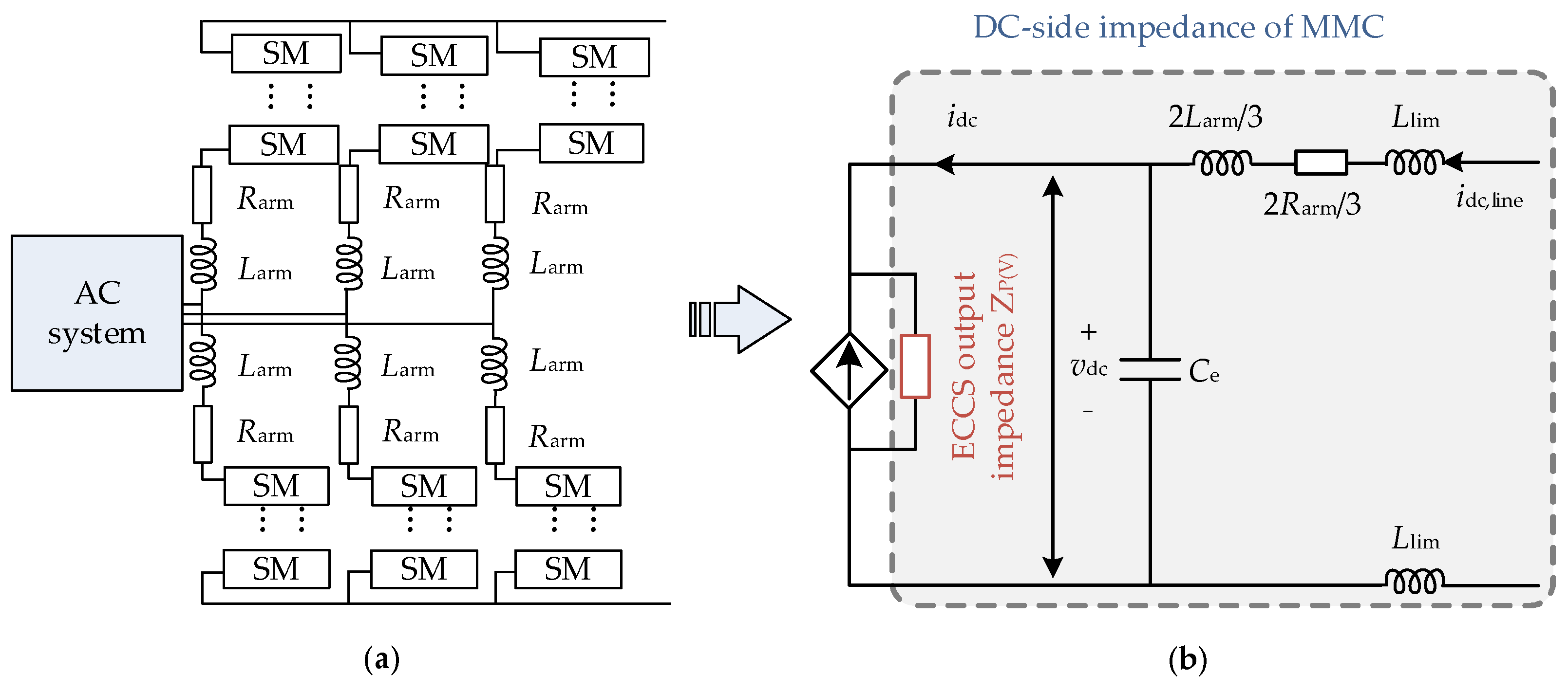
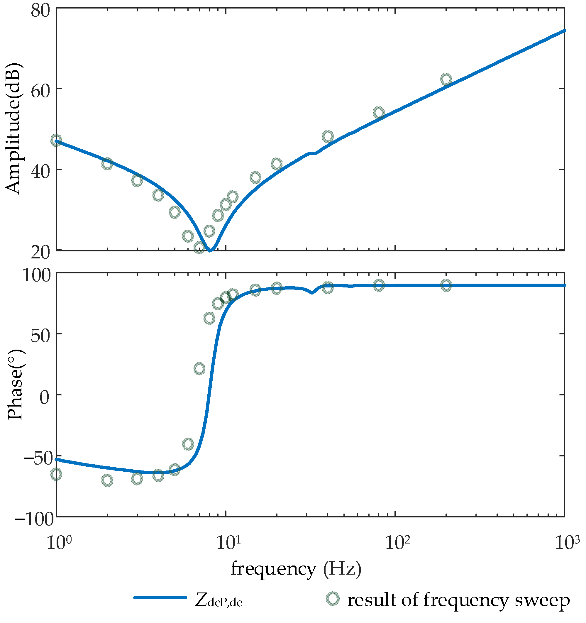
3.2. DC Side Impedance of MMC

The internal dynamic characteristics of the MMC are complex. To accurately describe its internal dynamic characteristics, high-order differential equations are required, which greatly increase the difficulty of modeling. When it comes to the external output characteristics of the MMC, the average value model of the MMC can be applied. Then, the model can ignore the charging and discharging processes of submodule capacitors and the influence of circulating currents between bridge arms, so the strategies of capacitor voltage equalization control and phase current circulating current suppression control can be omitted. This method can effectively reduce the complexity of the model while ensuring a certain degree of accuracy. The average value model of the MMC is shown in Figure 7, where L_arm and R_arm are the bridge arm inductance and bridge arm resistance, respectively, and C_e is the equivalent DC side capacitance, which can be expressed as

$$C_{\mathrm{e}}=6C_{\mathrm{sub}}/N$$

(13)

where N is the number of submodules and C_sub is the capacitance of each submodule.

In Figure 7, Z_P and Z_V are parallel equivalent impedances of equivalent controlled current sources (ECCSs) of the MMC with constant power control and voltage control, respectively. In Figure 6, the ECCS output impedances of MMC1 and MMC2 are Z₁ and Z₂, v_dc and i_dc are the voltage and current of the DC side of the ECCS, respectively, and i_dc,line is the DC output current of the MMC. The DC side impedance, which is obtained by taking the positive and negative terminals of a single converter station as ports, includes the ECCS output impedance, the DC equivalent capacitance, and the bridge arm impedance.

The ECCS output impedance of the MMC can be obtained from the relationship between DC voltage disturbance Δv_dc and DC current response Δi_dc. Specifically, the output power of the ECCS on the DC side is given by

$$P_{\mathrm{dc}}=v_{\mathrm{dc}}{i}_{\mathrm{dc}}$$

(14)

where P_dc0 is the rated DC active power.

Linearizing (14) obtains

$$\Delta i_{\mathrm{dc}}=\frac{\Delta P_{\mathrm{dc}}}{v_{\mathrm{dc}0}}-\frac{P_{\mathrm{dc}0}}{v_{\mathrm{dc}0}^2}\Delta v_{\mathrm{dc}}$$

(15)

To obtain the ECCS output impedance, which is the relationship between Δv_dc and Δi_dc, it is necessary to express ΔP_dc in terms of Δv_dc in (15). The power balance between the DC side and AC side of ECCS is given by

$$\Delta P_{\mathrm{dc}}=\Delta P_{\mathrm{ac}}$$

(16)

where P_ac is the active power on the AC side of the MMC, and its expression is given by

$$P_{\mathrm{a}\mathrm{c}}=\frac{3}{2}(u_{\mathrm{c}\mathrm{d}}{i}_{\mathrm{d}}+u_{\mathrm{c}\mathrm{q}}{i}_{\mathrm{q}})$$

(17)

After linearization near the steady-state operating point, the expression for the disturbance in P_ac can be obtained as

$$\Delta P_{\mathrm{ac}}=\frac{3}{2}\left[u_{\mathrm{c}d0}\hspace{0.33em}\hspace{0.33em}{u}_{\mathrm{c}q0}\right]\left[\begin{array}{l}\Delta i_d\\ \Delta i_q\end{array}\right]+\frac{3}{2}\left[i_{d0\hspace{0.33em}}\hspace{0.33em}{i}_{q0}\right]\left[\begin{array}{l}\Delta u_{\mathrm{c}d}\\ \Delta u_{\mathrm{c}q}\end{array}\right]$$

(18)

where u_cd0, u_cq0, i_d0, and i_q0 are the steady-state values of u_cd, u_cq, i_d, and i_q, respectively.

In summary, the key to establishing the ECCS output impedance is to obtain the relationship between Δv_dc and ΔP_ac. Based on the ECCS output impedance, the DC side impedance of the MMC can be easily calculated according to the MMC model in Figure 7.

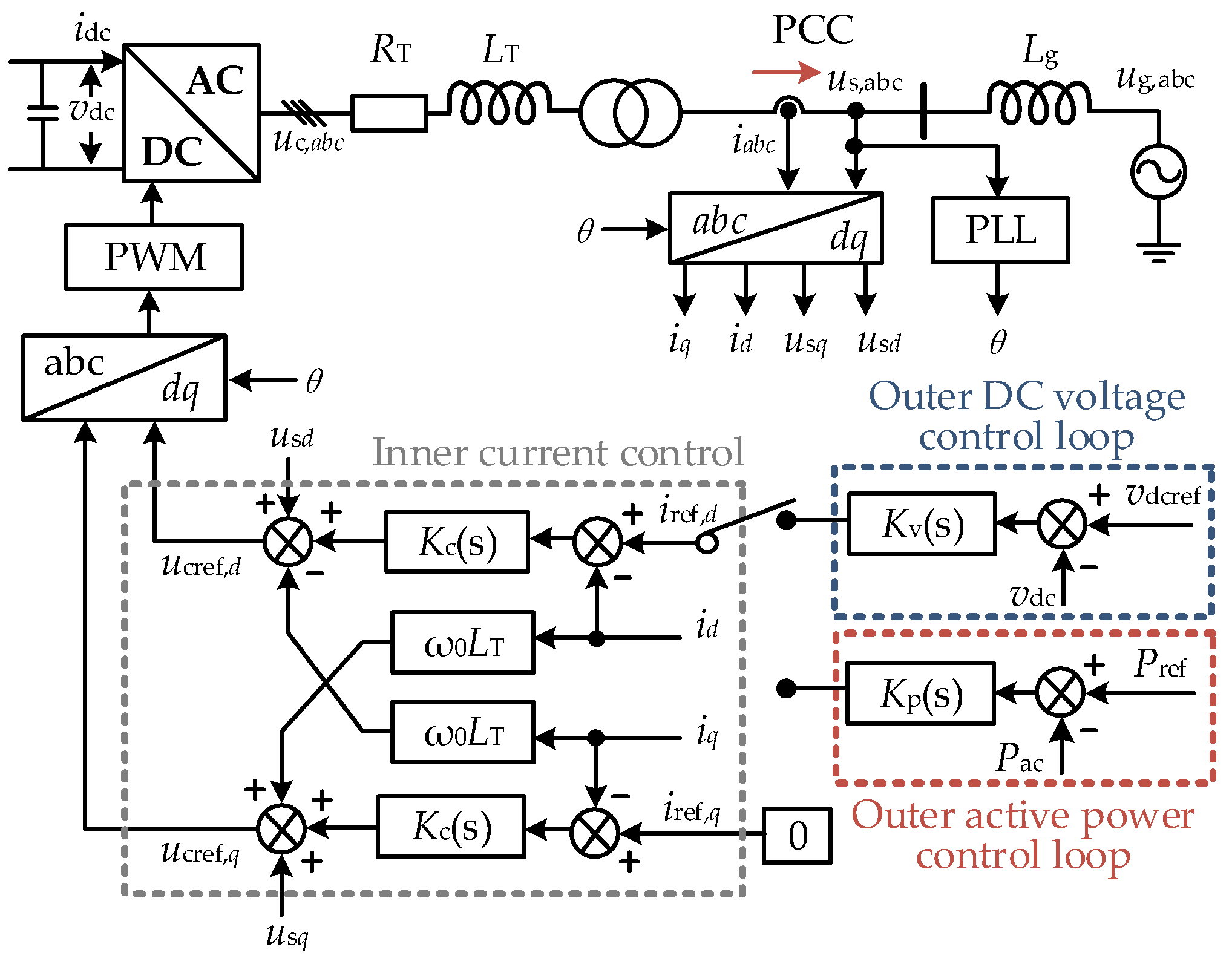
3.3. DC Side Impedance of MMC with Constant Power Control

The typical vector current control of the MMC is shown in Figure 8, where the DC voltage control and the constant power control are shown as the outer control loops. In Figure 8, u_g, u_s, and u_c are the voltage at the AC system bus, the point of common coupling (PCC), and the MMC AC output, respectively, P is the active power output of MMC, i is the AC current, L_g is the impedance of the AC system, L_T and R_T are the inductance and resistance of the transformer, respectively, θ is the phase of the PCC point voltage, ω₀ is the base frequency of the AC system, and K_v(s) and K_p(s) are the transfer functions of the PI loop for voltage control and power control, respectively. Moreover, the subscripts d, q, and abc indicate the variables of the d-axis, q-axis, and abc-frame, respectively, and the subscripts “ref” and “0” indicate the reference value and rated value of the variable. Since this paper focuses on the impact of frequency support control on the DC side stability of the MTDC, which is realized on the DC voltage control loop, the reactive power control loop is not considered, and the reactive current reference value i_ref,q is set to 0.

By derivation as shown in Appendix A, Z_P can be obtained as

$$\begin{array}{l}{Z}_{\mathrm{P},\mathrm{de}}=\frac{\Delta v_{\mathrm{dc}}}{\Delta i_{\mathrm{dc}}}=\\ -v_{\mathrm{dc}0}{\left(i_{\mathrm{dc}0}-\frac{3}{2}\left(-{\left[\begin{array}{c}{u}_{\mathrm{c}d0}\\ u_{\mathrm{c}q0}\end{array}\right]}^{\mathrm{T}}{\left(\begin{array}{l}{G}_{\mathrm{c}}{}^{-1}\left(G_{\mathrm{LT}}+Z_{\mathrm{T}}\right)+\\ \frac{3}{2}{K}_{\mathrm{p}}(s)(G_{\mathrm{u}0}-G_{\mathrm{i}0}{Z}_{\mathrm{T}})\end{array}\right)}^{-1}\left(\frac{3}{2}{K}_{\mathrm{p}}(s)G_{\mathrm{i}0}\right)+{\left[\begin{array}{c}{i}_{d0}\\ i_{q0}\end{array}\right]}^{\mathrm{T}}\right)\left[\begin{array}{l}{m}_{d0}\\ m_{q0}\end{array}\right]\right)}^{-1}\end{array}$$

(19)

Based on the average value model of the MMC as shown in Figure 7, in the impedance model of the MMC on the DC side, the equivalent output impedance of the ECCS is first connected in parallel with the equivalent capacitance C_e on the DC side, and then connected in series with the equivalent impedance L_arm and R_arm of the bridge arm. Based on the average value model of the MMC shown in Figure 7, the DC impedance Z_{dc_3} of the MMC station with constant active power control can be obtained as

$$Z_{\mathrm{dc}\text{\_}3}=\frac{Z_{\mathrm{P}}}{1+s{C}_{\mathrm{e}}{Z}_{\mathrm{P}}}+\frac{2}{3}(s{L}_{\mathrm{arm}}+R_{\mathrm{arm}})$$

(20)

Considering that MMC1 and MMC2, which connect OWF1 and OWF2, adopt island control, the expressions of the ECCS output impedances Z₁ and Z₂ for MMC1 and MMC2 are given by

$$Z_1=-\frac{v_{\mathrm{dc}0}^2}{P_1},Z_2=-\frac{v_{\mathrm{dc}0}^2}{P_2}$$

(21)

where P₁ and P₂ are the rated power of MMC1 and MMC2, respectively.

Similar to the analysis of the average model for the MMC above, the expressions of the DC side impedances Z_{dc_1} and Z_{dc_2} for MMC1 and MMC2 can be obtained as

$$\begin{array}{l}{Z}_{\mathrm{dc}\text{\_}1}=\frac{Z_1}{1+s{C}_{\mathrm{e}}{Z}_1}+\frac{2}{3}(s{L}_{\mathrm{arm}}+R_{\mathrm{arm}})\\ Z_{\mathrm{dc}\text{\_}2}=\frac{Z_2}{1+s{C}_{\mathrm{e}}{Z}_2}+\frac{2}{3}(s{L}_{\mathrm{arm}}+R_{\mathrm{arm}})\end{array}$$

(22)

3.4. DC Side Impedance of MMC with DC Voltage Control and Virtual Inertia Control

As shown in Figure 8, the control structure of the MMC with DC voltage control is the same as that with constant power control, except for the difference in the outer loop structure. K_v(s) is the PI controller for the voltage outer loop, which can be expressed as

$$K_{\mathrm{v}}(s)=k_{\mathrm{vp}}+k_{\mathrm{vi}}/s$$

(23)

where k_vp and k_vi are the proportional and integral parameters of the PI controller.

Since only the outer loop structure is changed for the MMC with DC voltage control, the inner loop structure, PWM structure, and AC system structure of the MMC output impedance model derived previously in the constant power control mode can still be used in the MMC with DC voltage control.

Based on the relationship between DC voltage disturbance Δv_dc, current disturbance Δi_dc, and power disturbance ΔP_dc shown in (15), the DC side output impedance of the MMC station under DC voltage control can be derived. According to the outer loop structure shown in Figure 8, the expression of the current reference for the current inner loop can be obtained as

$$\left[\begin{array}{l}{i}_{d\mathrm{ref}}\\ i_{q\mathrm{ref}}\end{array}\right]=\left[\begin{array}{l}{K}_{\mathrm{v}}(s)\\ \hspace{0.33em}\hspace{0.33em}\hspace{0.33em}0\end{array}\right](v_{\mathrm{dcref}}-v_{\mathrm{dc}})$$

(24)

Linearizing (24) near the operating point obtains

$$\left[\begin{array}{l}\Delta i_{d\mathrm{ref}}\\ \Delta i_{q\mathrm{ref}}\end{array}\right]=\left[\begin{array}{l}{K}_{\mathrm{v}}(s)\\ \hspace{0.33em}\hspace{0.33em}\hspace{0.33em}0\end{array}\right](\Delta v_{\mathrm{dcref}}-\Delta v_{\mathrm{dc}})$$

(25)

In order to provide inertia support to the AC system, frequency–voltage droop control is introduced into the outer control loop of the MMC with DC voltage control. This allows the reference value of the DC voltage to change with the system frequency, the expression is

$$v_{\mathrm{dcref}}=(f-f_{\mathrm{ref}})\cdot K_{\mathrm{DC}}+v_{\mathrm{dc}0}$$

(26)

where f is the real-time frequency of the system, f_ref is the reference frequency value, and K_DC is the droop coefficient.

Linearizing (26) near the equilibrium point obtains

$$\Delta v_{\mathrm{dcref}}=K_{\mathrm{DC}}\cdot \Delta f$$

(27)

According to the characteristics of the AC system in Figure 6, the relationship between frequency and power can be obtained by a genetic algorithm [30], as shown in (28).

$$\Delta f=G_{\mathrm{F}}(s)\frac{\Delta P}{s}=\frac{\Delta P(-0.1499\cdot s^3+32.58\cdot s^2+12.89\cdot s+1)}{s(270.3\cdot s^3+209.2\cdot s^2+96.34\cdot s+19.11)}$$

(28)

Introducing (28) into (27) obtains

$$\Delta v_{\mathrm{dcref}}=K_{\mathrm{DC}}\cdot G_{\mathrm{F}}(s)\frac{\Delta P}{s}=G_{\mathrm{P}}(s)\cdot \Delta P$$

(29)

where G_P(s) is

$$G_{\mathrm{P}}(s)=\frac{K_{\mathrm{DC}}\cdot (-0.1499\cdot s^3+32.58\cdot s^2+12.89\cdot s+1)}{s(270.3\cdot s^3+209.2\cdot s^2+96.34\cdot s+19.11)}$$

(30)

Substituting (29) into (25) obtains

$$\left[\begin{array}{l}\Delta i_{d\mathrm{ref}}\\ \Delta i_{q\mathrm{ref}}\end{array}\right]=\left[\begin{array}{l}{K}_{\mathrm{v}}(s)\\ \hspace{0.33em}\hspace{0.33em}\hspace{0.33em}0\end{array}\right](G_{\mathrm{P}}(s)\cdot \Delta P-\Delta v_{\mathrm{dc}})$$

(31)

By derivation as shown in Appendix B, Z_V can be obtained as

$$Z_{\mathrm{V}}=\frac{\Delta v_{\mathrm{dc}}}{\Delta i_{\mathrm{dc}}}=\frac{v_{\mathrm{dc}0}}{G_{\mathrm{V}}}$$

(32)

where

$$G_{\mathrm{V}}=\frac{3}{2}\left(\left[u_{\mathrm{c}d0}\hspace{0.33em}\hspace{0.33em}{u}_{\mathrm{c}q0}\right]\cdot G_{\mathrm{iv}}^{-1}\cdot G_{\mathrm{uv}}+\left[i_{d0}\hspace{0.33em}\hspace{0.33em}{i}_{q0}\right]\right)\left[\begin{array}{l}{m}_{d0}\\ m_{q0}\end{array}\right]+\frac{3}{2}\left[u_{\mathrm{c}d0}\hspace{0.33em}\hspace{0.33em}{u}_{\mathrm{c}q0}\right]\cdot G_{\mathrm{iv}}^{-1}\cdot G_{\mathrm{c}}\left[\begin{array}{l}{K}_{\mathrm{v}}(s)\\ \hspace{0.33em}\hspace{0.33em}\hspace{0.33em}0\end{array}\right]-i_{\mathrm{dc}0}$$

(33)

Based on the MMC average value model shown in Figure 7, the DC side impedance Z_{dc_4} of the MMC with DC voltage control can be obtained as

$$Z_{\mathrm{dc}\text{\_}4}=\frac{Z_{\mathrm{V}}}{1+s{C}_{\mathrm{e}}{Z}_{\mathrm{V}}}+\frac{2}{3}(s{L}_{\mathrm{arm}}+R_{\mathrm{arm}})$$

(34)

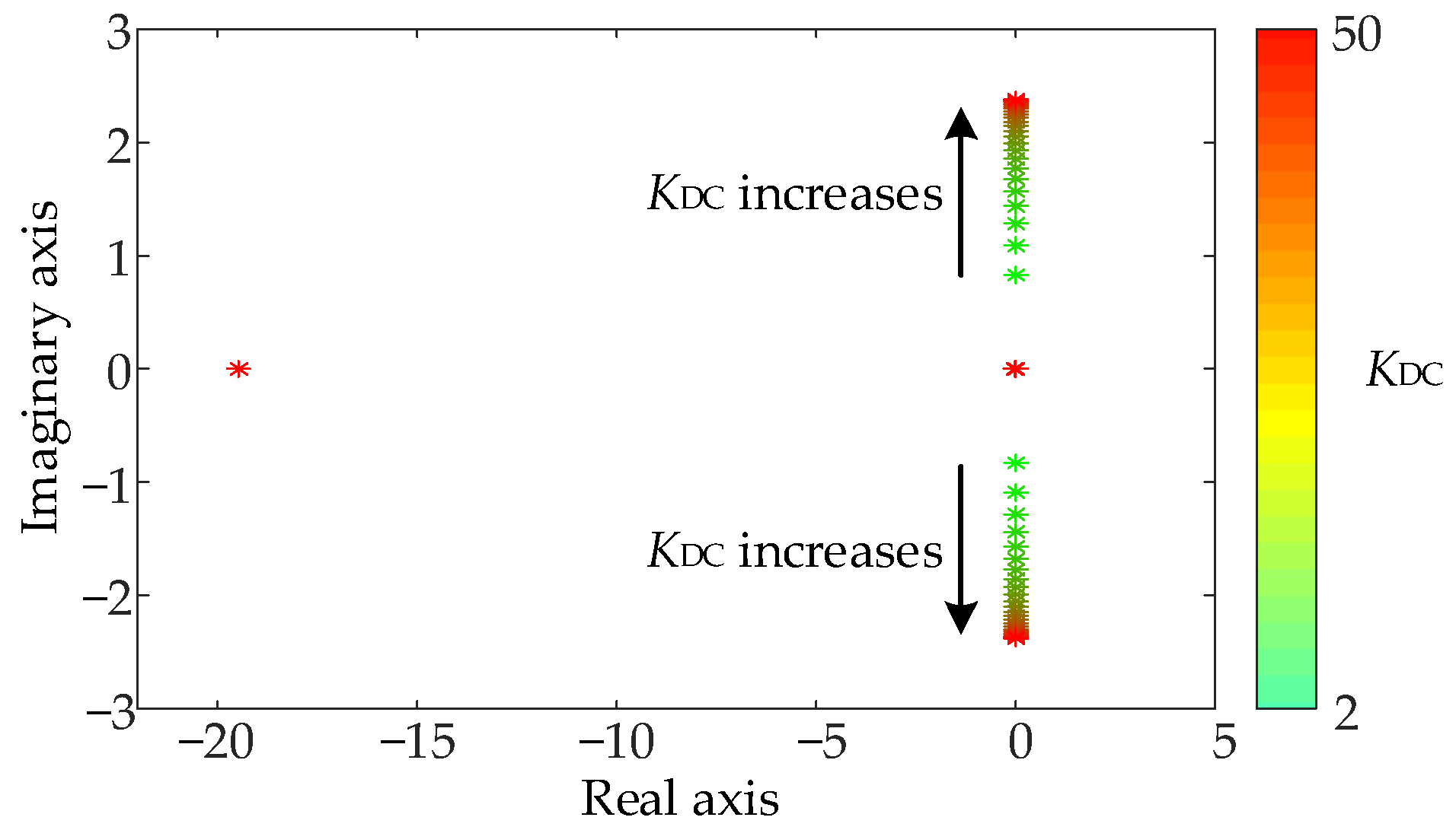
3.5. Impact of Frequency–Voltage Droop Coefficients on the Stability of MMC-MTDC System

The DC side impedance of each MMC in the MTDC system has been derived above. Taking the output of MMC2 as the port to evaluate the DC side stability of the MTDC system, after a simple series–parallel connection, the DC side impedance of the MMC-MTDC system is obtained as

$$Z_{\mathrm{sys}}=(Z_{\mathrm{dc}\text{\_}1}+Z_{12})//Z_{\mathrm{dc}\text{\_}1}+(Z_{\mathrm{dc}\text{\_}4}+Z_{34})//Z_{\mathrm{dc}\text{\_}2}+Z_{23}+L_{\lim }$$

(35)

To quantitatively analyze the DC side impedance of the MMC-MTDC system, a set of reference system parameters is required. The parameters of the four-terminal MMC-MTDC system shown in Figure 6 are listed in

Table 1. Electrical parameters of MMC-MTDC system.

Parameter	Value
Transformer load loss	0.006 pu
Transformer leakage reactance	0.18 pu
Number of submodules N	200
Submodule capacitance Csub	15 mF
Line equivalent resistance R12	0.25 Ω
Line equivalent inductance L12	2.5 mH
Line equivalent resistance R23	0.5 Ω
Line equivalent inductance L23	5 mH
Line equivalent resistance R34	0.4 Ω
Line equivalent inductance L34	4 mH
Current limiting inductor Llim	0.2 H
Arm resistance Rarm	0.15 Ω
Arm inductance Larm	30 mH

and

Table 2. Control parameters of MMC-MTDC system.

Parameter	Value
Frequency droop coefficient KDC	0.18 pu
PI transfer function of power outer loop Kp(s)	200
PI transfer function of current inner loop Kc(s)	15 mF
PI transfer function of voltage outer loop Kv(s)	0.25 Ω
Rated DC voltage vdc0	2.5 mH

.

The expression of the DC side impedance model of the MMC-MTDC system is given in (35). In order to verify the accuracy of Z_sys, a frequency sweep is performed on the MMC-MTDC system in PSCAD/EMTDC. The comparison between Z_sys and the simulation results of the frequency sweep in the simulation software is shown in Figure 9. As can be seen from Figure 9, Z_sys conforms well to the simulation frequency sweep results, and further analysis of the system stability can be conducted based on this.

Based on the four-terminal MMC-MTDC system structure as shown in Figure 6, combined with the DC side impedance expressions (20), (22), (34) of each converter station, as well as the overall DC side impedance expression (35) of the MMC-MTDC system and the benchmark system parameters in Table 1 and Table 2, the eigenvalue trajectory of Z_sys when the droop coefficient K_DC changes is obtained, and thus the impact of K_DC on the system stability can be analyzed.

In Figure 10, the system eigenvalue trajectory is shown when the droop coefficient K_DC changes from 2 to 50. It can be seen from the results that even when the droop coefficient K_DC increases to an almost exaggerated value, the system eigenvalues only remain distributed near the imaginary axis and do not cross over to the right half-plane. Therefore, even when the droop coefficient K_DC is increased to an exaggerated value, the system does not become unstable, and the impact of K_DC on the system stability is not significant within this wide range of variation.

4. Simulation Analysis

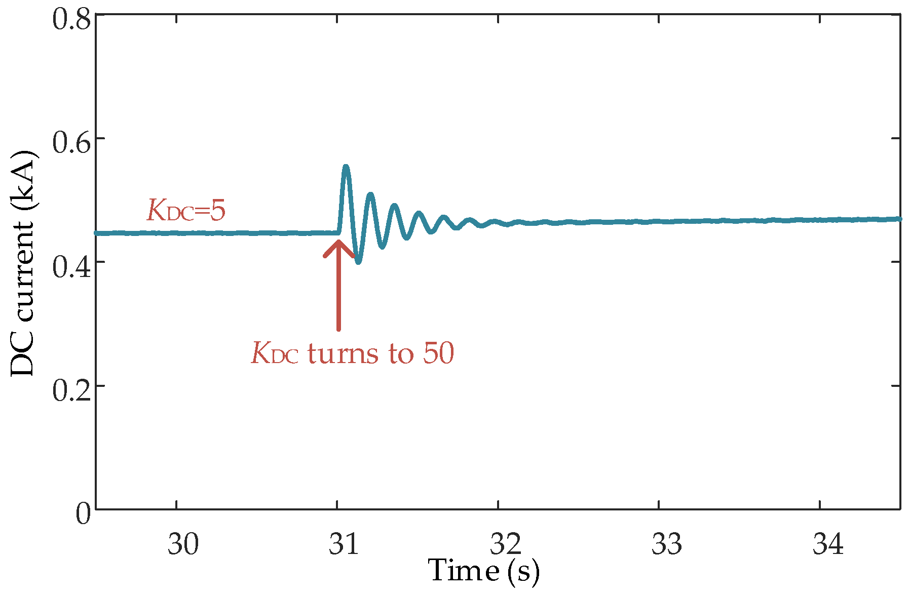
4.1. Verification of Impact of Droop Coefficient on MTDC System Stability

To verify the impact of the droop coefficient K_DC on system stability, a simulation model of the four-terminal MMC-MTDC system as shown in Figure 6 is constructed in PSCAD/EMTDC. The simulation result is shown in Figure 11. When the droop coefficient K_DC is increased from 5 to 50 at 31 s, the system quickly regains stability after a short period of fluctuation and does not become unstable, which validates the stability analysis results. It can be concluded that even if the droop coefficient K_DC is increased significantly to 50, the system will not become unstable. Therefore, the impact of droop coefficient K_DC on MTDC system stability is not significant. When the frequency–voltage droop coefficient K_DC is adjusted, its impact on the overall stability of the MTDC system can be neglected.

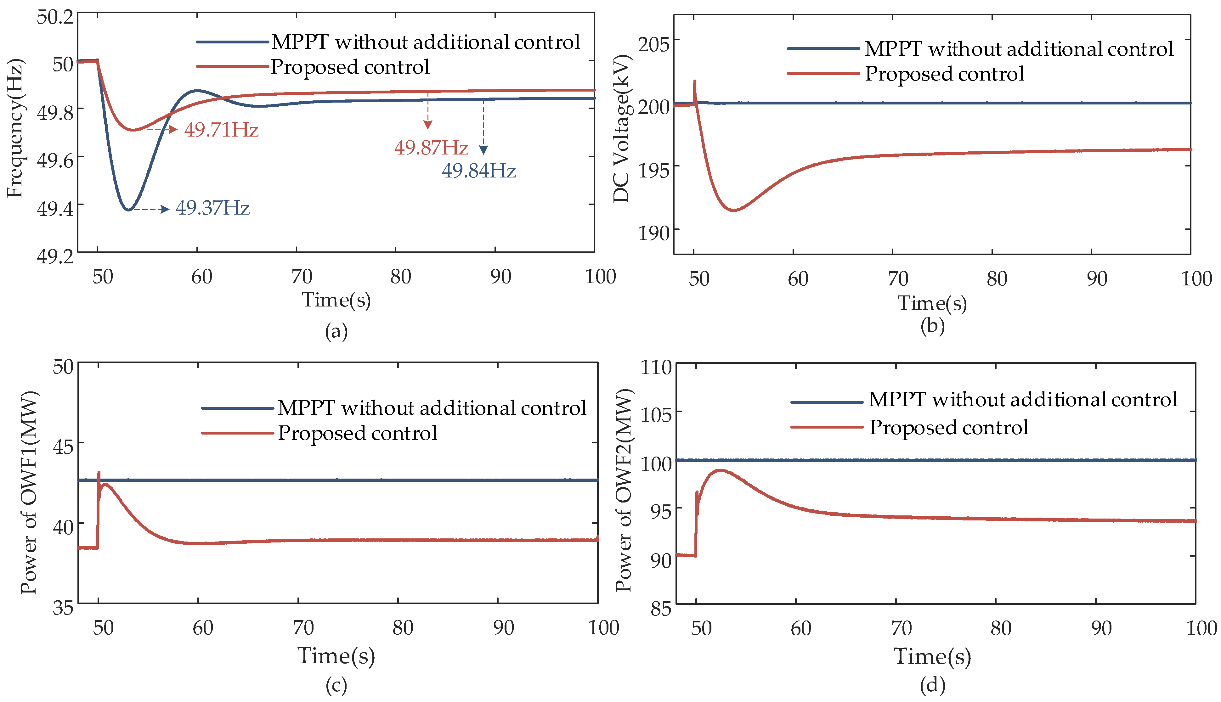
4.2. Validation of Frequency Support Effect of OWF-MTDC

To validate the frequency support effect of the proposed control method under load disturbance, the MMC-MTDC system integrating OWFs shown in Figure 6 was constructed in PSCAD/EMTDC. The onshore IEEE 3-machine 9-bus system consists of a hydro generator G1 with IEEE G3 type speed governing system and steam generators G2, G3 with IEEE G1 type speed governing systems. The parameters of the WTGS and AC system are shown in

Table 3. Main parameters of WTGS.

Parameter	Value
Rated power SWT	2 MW
Number of WTGSs in a single OWF	50
Rated frequency fN	50 Hz
Terminal voltage	0.69 kV
Rated rotor speed ω	1.2 pu
Power reserve coefficient d%	10%
Wind speed of OWF1	8 m/s
Wind speed of OWF2	13 m/s
Virtual inertia of OWF1 H1	5 s
Virtual inertia of OWF2 H2	7 s
Power droop coefficient of OWF1 KP1	7
Power droop coefficient of OWF2 KP2	15

and

Table 4. Main parameters of AC system.

Parameter	Value
Rated power of G1 SG1	72 MW
Rated power of G2 SG2	163 MW
Rated power of G3 SG3	85 MW
Inertia time constant of G1 HG1	8 s
Inertia time constant of G2 HG2	6.4 s
Inertia time constant of G3 HG3	3.01 s

, respectively. From the above impedance analysis, the droop coefficient K_DC does not obviously affect the MTDC system stability. Thus, K_DC can be determined based on the frequency deviation and allowable voltage deviation. Considering the power grid operation specification, the frequency deviation Δf of the power system is generally controlled within 2% (1 Hz), and the DC voltage deviation Δv_dc is set within 15% [31]. Therefore, the droop coefficient K_DC in this paper is set to 7.5. A sudden load step of 5% was set at 50 s, and the simulation results under MPPT without additional control and the proposed control method are shown in Figure 12.

As shown in Figure 12, the WTGS without additional control always operates at the maximum power point and does not respond to the onshore grid frequency deviation, where the frequency nadir is 49.37 Hz and the steady state frequency is 49.84 Hz under the disturbance. When the MTDC system adopts the proposed control method, the OWFs reserve 10% of their maximum available power, i.e., OWF1 reserves 4.3 MW and OWF2 reserves 10 MW. After the load step, the rotor kinetic energy and reserved power of the WTGSs are quickly released, and the additional output power provides virtual inertia and damping to the AC system for frequency support. The additional power is correlated with the reserve power, as shown in Figure 12c,d. Moreover, the MMC provides virtual inertia to the AC system by the DC capacitor, and the DC voltage deviation is positively correlated with the frequency deviation. Specifically, the maximum DC voltage deviation does not exceed 10%, as shown in Figure 12b, indicating that the droop coefficient is set appropriately. With the proposed control method, the frequency nadir is 49.71 Hz, and the maximum frequency deviation is reduced by 53.97% compared with the case without frequency support control, and the steady-state frequency is 49.87 Hz, which is 0.03 Hz higher than the case without frequency support control. In summary, the proposed control method can effectively provide frequency support to the onshore AC system without affecting the stability of the WTGSs and the MTDC system.

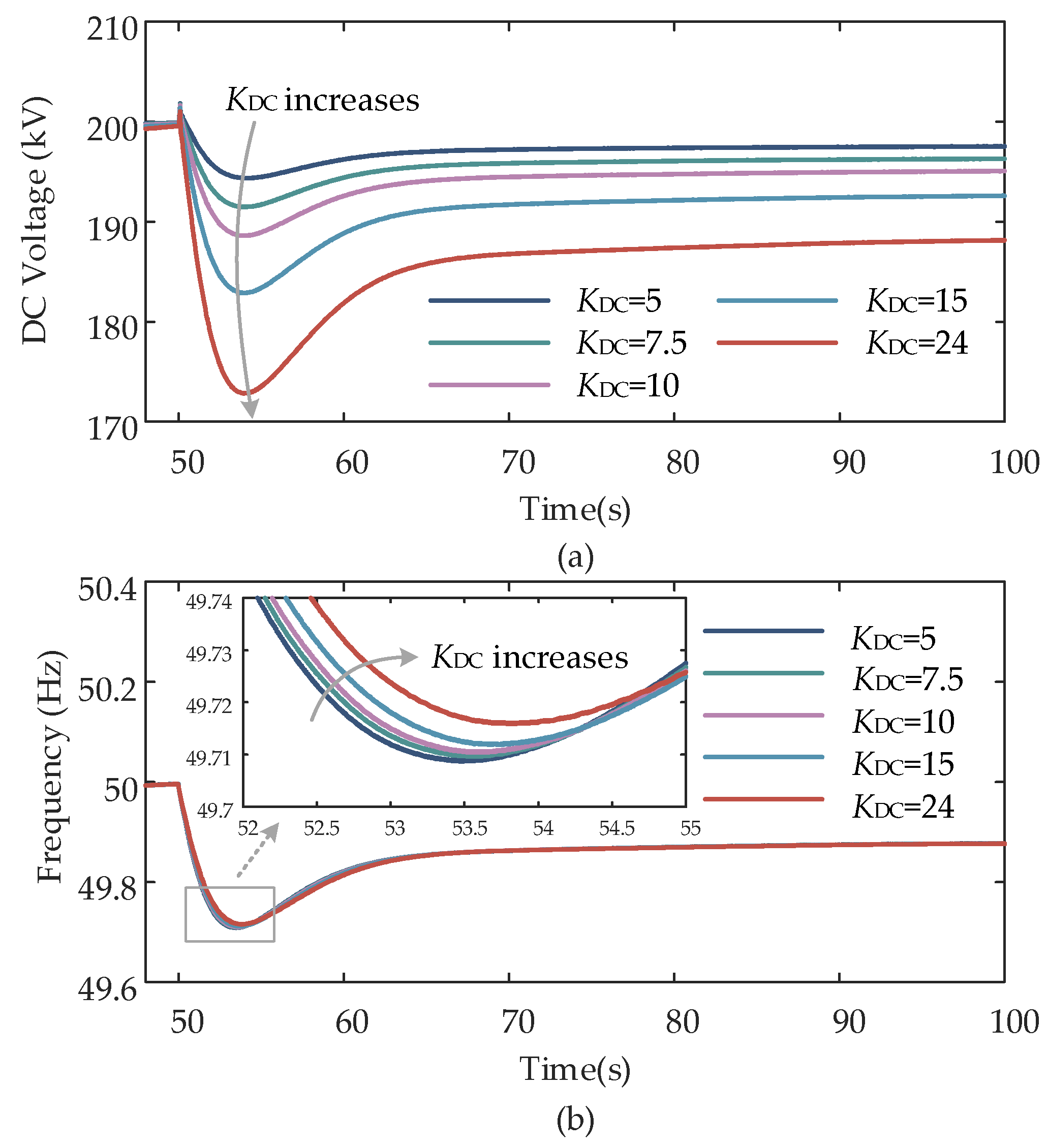
4.3. Simulation Results with Different Frequency–Voltage Droop Coefficients

In order to verify the impact of the frequency–voltage droop coefficient on the MTDC system stability as discussed in Section 3, the cases with different K_DC are conducted. The simulation results of DC voltage and frequency with different K_DC under a 5% sudden load step at 50 s are shown in Figure 13.

It can be seen in Figure 13 that the increase in frequency–voltage droop coefficient does not affect the stability of the system, verifying the stability analysis in Section 3. As K_DC increases, the DC capacitor releases more energy, making the DC voltage drop more severely, which then raises the frequency nadir. This indicates that the virtual inertia control of the MMC can effectively provide frequency support to the onshore AC system, of which the performance is determined by the droop coefficient K_DC. Considering that the voltage deviation should be kept within 30 kV, the maximum value of K_DC is set to 24. However, since the voltage deviation is directly related to the frequency deviation, if the power droop coefficients of WTGSs are increased, the frequency nadir can be significantly increased, and the maximum value of K_DC can also be correspondingly increased.

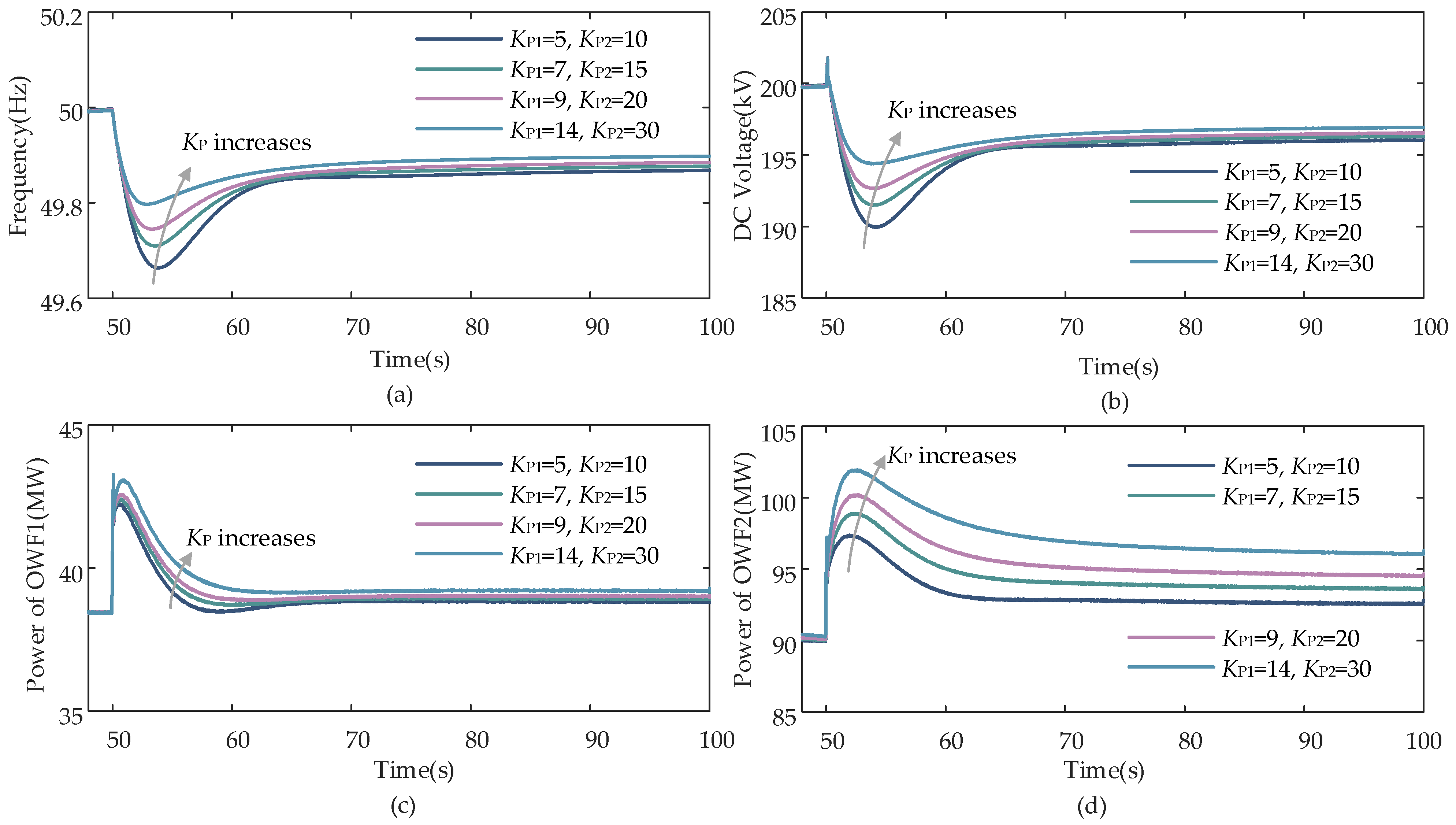
4.4. Simulation Results with Different Power Droop Coefficients

In order to investigate the influence of the wind turbine power droop coefficient K_P (including droop coefficient of OWF1 K_P1 and the droop coefficient of OWF2 K_P2) on the system, several sets of power droop coefficients were added while keeping the GSVSC frequency–voltage droop coefficient K_DC fixed at 7.5. The simulation results under each parameter with a 5% sudden load step at 50 s are shown in Figure 14. It can be seen from Figure 14 that the WTGS power droop control has a significant frequency raising effect. As K_P increases, the OWFs output more additional power after the frequency event, and the frequency nadir of the AC system is raised while the steady-state frequency deviation is reduced. Since the DC voltage under the virtual inertia control of the DC capacitor is directly related to the frequency, the DC voltage is also raised. Therefore, under the premise of increasing the WTGS power droop coefficient, a higher frequency–voltage droop coefficient can be set within the allowable range of DC voltage deviation, which can further raise the lowest frequency point of the AC system. At the same time, it can be seen from the simulation results that changing the WTGS droop coefficient only affects the frequency support effect and does not affect the system stability. Therefore, the DC impedance modeling in Section 3 is reasonable for the simplification of MMC1 and MMC2 and does not affect the stability analysis results.

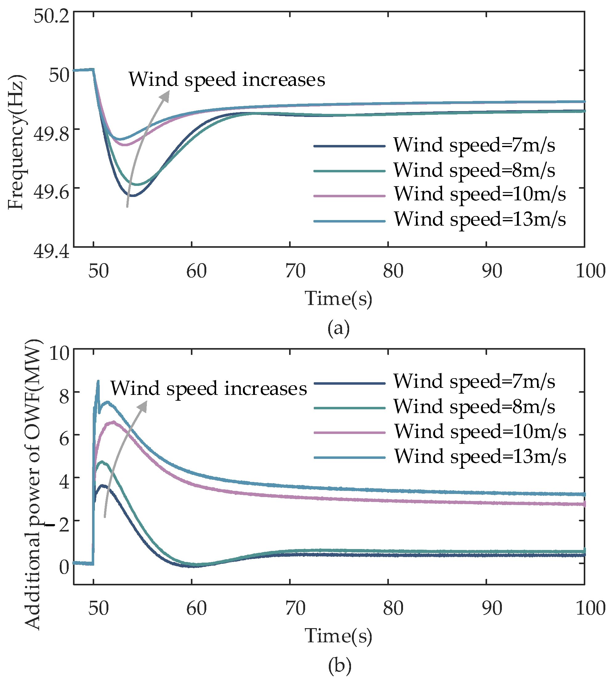
4.5. Simulation Results with Different Wind Speeds

The wind speed exhibits variability during actual operation. To evaluate the effectiveness of the proposed method across a range of wind speeds, simulation tests are conducted for OWFs with different wind speeds. WTGSs operating under low wind speeds are unsuitable for power reserve purposes. Conversely, when the wind speed surpasses the rated value, the rotor speed and output power remain constant at the rated level. In this case study, wind speeds of 7 m/s, 8 m/s, 10 m/s, and 13 m/s are selected for all the OWFs. The frequency–voltage droop coefficient K_DC of the GSVSC is fixed at 7.5, while the virtual inertia constant H and the frequency–power droop coefficient K_P are determined based on (4) and (5). Figure 15 illustrates the simulation results under different wind speeds, where subfigure (b) represents the additional output power of a single OWF with different wind speeds. To assess system performance, a sudden 5% load step is applied at 50 s.

As it can be seen from the results, the rotor speed and reserve power increase with wind speed, thereby the virtual inertia constant and droop coefficient are increased. Then, with a higher wind speed, the frequency nadir under the same disturbance was raised, as shown in Figure 15a, and the additional output power of OWF increases, as shown in Figure 15b. The simulation results prove that the proposed method can flexibly adjust the control coefficients according to the real-time wind speed, leading to improved frequency support performance, and the WTGSs can operate stably in the allowed wind speed range.

5. Conclusions

This paper proposes a frequency support control method for an OWF-MTDC system based on the DC side stability analysis of the MTDC system. For the WTGSs with power reserve, the rotor virtual inertia control and frequency–power droop control are designed to enable frequency regulation. For the MTDC system, the frequency–voltage droop control is designed for the MMC to provide virtual inertia by the use of the DC capacitor. The detailed DC side impedance of the MTDC system is modeled considering the MMCs under constant power control and DC voltage control. The effect of frequency–voltage droop coefficient on the MTDC system stability is then investigated based on the model, of which the results show that the proposed frequency support control is tolerant of control coefficients in terms of stability consideration. The proposed control method enables the WTGSs and the MTDC system to respond to onshore grid frequency fluctuation in a timely manner, providing additional frequency support to the onshore AC system. Simulation results show that the proposed method can reduce the maximum frequency deviation of the system by 53.97% and raises the steady-state frequency by 0.03 Hz under a disturbance. By changing the frequency–voltage droop coefficient of the MMC and the power droop coefficient of the WTGSs, the system stability is not affected, verifying the stability analysis results. The simulation results with different wind speeds prove that the proposed method can flexibly adjust the control coefficients according to the wind speed, leading to improved frequency support performance. In summary, the proposed method has a fast response speed and great frequency support performance, which effectively improves the inertia and damping coefficient of the power system and further enhances the frequency stability of the onshore power grid. In future work, we will study the time sharing coordination of virtual inertia control and droop control to further improve the frequency support performance.

References

1. Wang, W.Y.; Li, Y.; Cao, Y.J.; Hager, U.; Rehtanz, C. Adaptive droop control of VSC-MTDC system for frequency support and power sharing. IEEE Trans. Power Syst. 2018, 33, 1264–1274. [Google Scholar] [CrossRef]
2. Peng, Q.; Liu, T.Q.; Wang, S.L.; Qiu, Y.F.; Li, X.Y.; Li, B.H. Determination of droop control coefficient of multi-terminal VSC-HVDC with system stability consideration. IET Renew. Power Gener. 2018, 12, 1508–1515. [Google Scholar] [CrossRef]
3. Sun, K.; Yao, W.; Fang, J.K.; Ai, X.M.; Wen, J.Y.; Cheng, S.J. Impedance modeling and stability analysis of grid-connected DFIG-based wind farm with a VSC-HVDC. IEEE J. Emerg. Sel. Top. Power Electron. 2020, 8, 1375–1390. [Google Scholar] [CrossRef]
4. Xiong, Y.X.; Yao, W.; Wen, J.F.; Lin, S.Q.; Ai, X.M.; Fang, J.K.; Wen, J.Y.; Cheng, S.J. Two-level combined control scheme of VSC-MTDC integrated offshore wind farms for onshore system frequency support. IEEE Trans. Power Syst. 2021, 36, 781–792. [Google Scholar] [CrossRef]
5. Wang, Y.; Nguyen, T.L.; Xu, Y.; Li, Z.M.; Tran, Q.-T.; Caire, R. Cyber-physical design and implementation of distributed event-triggered secondary control in islanded microgrids. IEEE Trans. Ind. Appl. 2019, 55, 5631–5642. [Google Scholar] [CrossRef]
6. Li, Y.S.; Zhang, H.G.; Liang, X.D.; Huang, B.N. Event-triggered-based distributed cooperative energy management for multienergy systems. IEEE Trans. Ind. Inform. 2019, 15, 2008–2022. [Google Scholar] [CrossRef]
7. Guan, M.Y. Scheduled power control and autonomous energy control of grid-connected energy storage system (ESS) with virtual synchronous generator and primary frequency regulation capabilities. IEEE Trans. Power Syst. 2022, 37, 942–954. [Google Scholar] [CrossRef]
8. Li, Z.; Wei, Z.A.; Zhan, R.P.; Li, Y.Z.; Tang, Y.; Zhang, X.-P. Frequency support control method for interconnected power systems using VSC-MTDC. IEEE Trans. Power Syst. 2021, 36, 2304–2313. [Google Scholar] [CrossRef]
9. Xu, B.; Zhang, L.W.; Yao, Y.; Yu, X.D.; Yang, Y.X.; Li, D.D. Virtual inertia coordinated allocation method considering inertia demand and wind turbine inertia response capability. Energies 2021, 14, 5002. [Google Scholar] [CrossRef]
10. Jiang, Q.; Zeng, X.Y.; Li, B.H.; Wang, S.L.; Liu, T.Q.; Chen, Z.; Wang, T.X.; Zhang, M. Time-sharing frequency coordinated control strategy for PMSG-based wind turbine. IEEE J. Emerg. Sel. Topics Circuits Syst. 2022, 12, 268–278. [Google Scholar] [CrossRef]
11. Zeng, X.Y.; Liu, T.Q.; Wang, S.L.; Dong, Y.Q.; Li, B.H.; Chen, Z. Coordinated control of MMC-HVDC system with offshore wind farm for providing emulated inertia support. IET Renew. Power Gener. 2020, 14, 673–683. [Google Scholar] [CrossRef]
12. Xiong, Y.X.; Yao, W.; Yao, Y.H.; Fang, J.K.; Ai, X.M.; Wen, J.Y.; Cheng, S.J. Distributed cooperative control of offshore wind farms integrated via MTDC system for fast frequency support. IEEE Trans. Ind. Electron. 2023, 70, 4693–4704. [Google Scholar] [CrossRef]
13. Kheshti, M.; Lin, S.Y.; Zhao, X.W.; Ding, L.; Yin, M.H.; Terzija, V. Gaussian distribution-based inertial control of wind turbine generators for fast frequency response in low inertia systems. IEEE Trans. Sustain. Energy 2022, 13, 1641–1653. [Google Scholar] [CrossRef]
14. Tu, G.G.; Li, Y.J.; Xiang, J. Coordinated rotor speed and pitch angle control of wind turbines for accurate and efficient frequency response. IEEE Trans. Power Syst. 2022, 37, 3566–3576. [Google Scholar] [CrossRef]
15. Wang, X.; He, Y.G.; Gao, D.W.; Wang, Z.Y.; Muljadi, E. Cooperative output regulation of large-scale wind turbines for power reserve control. IEEE Trans. Energy Convers. 2023, 38, 1166–1177. [Google Scholar] [CrossRef]
16. Ge, X.L.; Zhu, X.H.; Fu, Y.; Xu, Y.S.; Huang, L.L. Optimization of reserve with different time scales for wind-thermal power optimal scheduling considering dynamic deloading of wind turbines. IEEE Trans. Sustain. Energy 2022, 13, 2041–2050. [Google Scholar] [CrossRef]
17. Peng, Q.; Jiang, Q.; Yang, Y.H.; Liu, T.Q.; Wang, H.; Blaabjerg, F. On the stability of power electronics-dominated systems: Challenges and potential solutions. IEEE Trans. Ind. Appl. 2019, 55, 7657–7670. [Google Scholar] [CrossRef]
18. Kou, P.; Liang, D.L.; Wu, Z.H.; Ze, Q.J.; Gao, L. Frequency support from a DC-grid offshore wind farm connected through an HVDC link: A communication-free approach. IEEE Trans. Energy Convers. 2018, 33, 1297–1310. [Google Scholar] [CrossRef]
19. Peng, Q.; Fang, J.Y.; Yang, Y.H.; Liu, T.Q.; Blaabjerg, F. Maximum virtual inertia from DC-link capacitors considering system stability at voltage control timescale. IEEE J. Emerg. Sel. Topics Circuits Syst. 2021, 11, 79–89. [Google Scholar] [CrossRef]
20. Xu, Z.G.; Li, B.B.; Han, L.J.; Hu, J.L.; Wang, S.B.; Zhang, S.G.; Xu, D.G. A complete HSS-based impedance model of MMC considering grid impedance coupling. IEEE Trans. Power Electron. 2020, 35, 12929–12948. [Google Scholar] [CrossRef]
21. Hu, J.B.; Zhu, J.H.; Wan, M. Modeling and analysis of modular multilevel converter in DC voltage control timescale. IEEE Trans. Ind. Electron. 2019, 66, 6449–6459. [Google Scholar] [CrossRef]
22. Lyu, J.; Zhang, X.; Cai, X.; Molinas, M. Harmonic state-space based small-signal impedance modeling of a modular multilevel converter with consideration of internal harmonic dynamics. IEEE Trans. Power Electron. 2019, 34, 2134–2148. [Google Scholar] [CrossRef] [Green Version]
23. Lyu, J.; Zhang, X.; Huang, J.J.; Zhang, J.W.; Cai, X. Comparison of harmonic linearization and harmonic state space methods for impedance modeling of modular multilevel converter. In Proceedings of the 2018 International Power Electronics Conference (IPEC), Niigata, Japan, 20–24 May 2018; pp. 1004–1009. [Google Scholar]
24. Li, C.; Cao, Y.J.; Yang, Y.Q.; Wang, L.; Blaabjerg, F.; Dragicevic, T. Impedance-based method for DC stability of VSC-HVDC system with VSG control. Int. J. Electr. Power Energy Syst. 2021, 130, 106975. [Google Scholar] [CrossRef]
25. Agbemuko, A.J.; Domínguez-García, J.L.; Prieto-Araujo, E.; Gomis-Bellmunt, O. Impedance modelling and parametric sensitivity of a VSC-HVDC system: New insights on resonances and interactions. Energies 2018, 11, 845. [Google Scholar] [CrossRef] [Green Version]
26. Amin, M.; Molinas, M.; Lyu, J.; Cai, X. Impact of power flow direction on the stability of VSC-HVDC seen from the impedance nyquist plot. IEEE Trans. Power Electron. 2017, 32, 8204–8217. [Google Scholar] [CrossRef]
27. Paul, S.; Rather, Z.H. A novel approach for optimal cabling and determination of suitable topology of MTDC connected offshore wind farm cluster. Electr. Power Syst. Res. 2022, 208, 107877. [Google Scholar] [CrossRef]
28. Li, Y.J.; Xu, Z.; Zhang, J.L.; Yang, H.M.; Wong, K.P. Variable utilization-level scheme for load-sharing control of wind farm. IEEE Trans. Energy Convers. 2018, 33, 856–868. [Google Scholar] [CrossRef]
29. Dreidy, M.; Mokhlis, H.; Mekhilef, S. Inertia response and frequency control techniques for renewable energy sources: A review. Renew. Sust. Energ. Rev. 2017, 69, 144–155. [Google Scholar] [CrossRef]
30. Huang, H.; Ju, P.; Jin, Y.; Yuan, X.; Qin, C.; Pan, X.; Zang, X. Generic system frequency response model for power grids with different generations. IEEE Access 2020, 8, 14314–14321. [Google Scholar] [CrossRef]
31. Zhu, J.B.; Hu, J.B.; Huang, W.; Wang, C.S.; Zhang, X.; Bu, S.Q.; Li, Q.; Urdal, H.; Booth, C.D. Synthetic inertia control strategy for doubly fed induction generator wind turbine generators using lithium-ion supercapacitors. IEEE Trans. Energy Convers. 2018, 33, 773–783. [Google Scholar] [CrossRef]
Figure 1. OWF-MTDC system configuration.
Electronics 12 03029 g001
Figure 2. MPPT curve and d% reserved power curve.
Electronics 12 03029 g002
Figure 3. Diagram of the additional power control with frequency support.
Electronics 12 03029 g003
Figure 4. Virtual inertia control of MMC.
Electronics 12 03029 g004
Figure 5. Flow chart of the frequency control of OWF-MTDC system.
Electronics 12 03029 g005
Figure 6. Topology of the four-terminal OWF-MTDC system.
Electronics 12 03029 g006
Figure 7. Structure and average value model of MMC: (a) structure of MMC; (b) average value model of MMC.
Electronics 12 03029 g007
Figure 8. Typical vector current control system of MMC.
Electronics 12 03029 g008
Figure 9. Comparison between Zsys and simulation results.
Electronics 12 03029 g009
Figure 10. System eigenvalue trajectory when KDC changes.
Electronics 12 03029 g010
Figure 11. Simulation results of the impact of KDC on MTDC system stability.
Electronics 12 03029 g011
Figure 12. Simulation results of OWF-MTDC system under a 5% sudden load step: (a) frequency variation of AC system, (b) DC voltage variation of MTDC system, (c) output power of OWF1, and (d) output power of OWF2.
Electronics 12 03029 g012
Figure 13. Simulation results of OWF-MTDC system with different frequency–voltage droop coefficients: (a) DC voltage variation of MTDC system and (b) frequency variation of AC system.
Electronics 12 03029 g013
Figure 14. Simulation results with different power droop coefficients: (a) frequency variation of AC system; (b) DC voltage variation of MTDC system; (c) output power of OWF1; (d) output power of OWF2.
Electronics 12 03029 g014
Figure 15. Simulation results with different wind speeds: (a) Frequency variation of AC system; (b) additional output power of OWF.
Electronics 12 03029 g015