Robust Adaptive Beamforming Based on a Convolutional Neural Network

Abstract

To address the advancements in jamming technology, it is imperative to consider robust adaptive beamforming (RBF) methods with finite snapshots and gain/phase (G/P) errors. This paper introduces an end-to-end RBF approach that utilizes a two-stage convolutional neural network. The first stage includes convolutional blocks and residual blocks without downsampling; the blocks assess the covariance matrix precisely using finite snapshots. The second stage maps the first stage’s output to an adaptive weight vector employing a similar structure to the first stage. The two stages are pre-trained with different datasets and fine-tuned as end-to-end networks, simplifying the network training process. The two-stage structure enables the network to possess practical physical meaning, allowing for satisfying performance even with a few snapshots in the presence of array G/P errors. We demonstrate the resulting beamformer’s performance with numerical examples and compare it to various other adaptive beamformers.

1. Introduction

Adaptive digital beamforming (ADBF) has found extensive applications in various fields such as radar, sonar, speech processing, etc., as it enhances the desired signal (signal-of-interest or SoI) while suppressing interference (signal of avoidance or SoAs) at the array output [1,2,3,4,5]. The minimum variance distortionless response (MVDR) beamformer is a popular adaptive beamformer that adaptively selects the weight vector to minimize the array output power, subject to the linear constraint that the target signal remains undistorted [6]. However, the MVDR beamformer’s performance degrades significantly with imprecise knowledge of steering vectors and insufficient available snapshots, requiring the use of more robust beamforming (RBF) techniques in practical applications [7].

Over the years, several studies have been conducted to introduce an effective RBF method. There are three primary categories of RBF techniques.

• Diagonal loading methods [8] augment the sample covariance matrix (SCM) with a coefficient-scaled identity matrix to enhance the system’s robustness to SoI mismatches and the finite snapshot effect. However, these methods require determining the optimal diagonal loading factor in various scenarios, which remains challenging.
• Feature subspace projection-based RBF [9,10], which projects the SoI steering vector onto both the noise and signal plus interference subspaces to mitigate interference. However, this method may struggle at differentiating between subspaces when the signal to interference plus noise ratio (SINR) is low.
• Convex optimization-based RBF extends the diagonal loading technique by obtaining the diagonal loading factor through an optimization problem. Different approaches have been proposed, including minimizing a quadratic function with non-convex quadratic constraints [11], shrinking the unbiased SCM [12], employing an iterative method to reduce the estimation error of the SCM [13], and obtaining the diagonal loading factor adaptively via a shrinkage method [14]. However, these methods often have a gap in output SINR compared to the optimal SINR and do not directly relate the adaptive weight vector to the scene’s error [15].

Additionally, there is another type of RBF method that reconstructs the interference plus a noise covariance matrix from the signal using a spectral estimator, effectively eliminating the target component in the SCM [16,17,18,19,20,21].

The neural network boasts robust nonlinear fitting abilities, thereby being extensively utilized to tackle optimization problems. Deep learning (DL) has showcased promising potential in radar signal processing encompassing radar imaging [22], spectral estimation [23], space-time adaptive processing [24], and radar target recognition [25]. In fact, researchers have made attempts to leverage DL techniques for ADBF, as evidenced by relevant literature. In [26], the application of a deep convolutional neural network (CNN) to adaptive beamforming resulted in a reduction in computation time. The proposed network inputs an image-like radiation pattern that encodes the desired behavior, subsequently computing the optimal currents necessary to adapt the antenna to the new beam specification. Furthermore [27], presented a deep neural network (DNN) that efficiently learns to perform fast and high-quality ultrasound beamforming using only a few snapshots. The proposed framework holds promise for a range of array and signal processing applications, particularly in scenarios where data efficiency and robustness play crucial roles. In [28], a data-driven method was proposed for designing sparse array configurations that maximize SINR in a narrowband interfering environment. Through various design examples, it was demonstrated that the DNN-based method enables efficient real-time implementation. Similarly [29], employed a recurrent neural network based on the gated recurrent unit architecture to serve as a beamformer, generating appropriate complex weights to feed into the antenna array. Meanwhile, in [30], a DL-based approach that utilizes a deep 1D complex-valued convolutional neural network (CVCNN) was proposed to compute an almost optimal beamformer. In [31], the authors proposed a data-driven model employing the Bat algorithm in conjunction with the general regression neural network (GRNN) to address the wide nulling challenges encountered in an ADBF array. These studies highlight how DL-based ADBF techniques are feasible. However, there exist some common and noteworthy limitations. For instance, the data utilized by these approaches to training neural networks typically consist of beam patterns or spatial spectra instead of raw echoes, which incur additional computational costs and information loss. Additionally, factors such as G/P errors have yet to be taken into account. Furthermore, the effect of finite available snapshots on the DL-based ADBF methods has not yet been studied in depth.

This paper proposes an end-to-end RBF method with a unique CNN structure to address the aforementioned issues. The proposed network features a two-stage factored structure, where each stage serves a distinct function and holds physical significance. The first stage, involving several convolutional blocks and residual blocks without downsampling, accurately estimates the SCM using finite snapshots. The second stage then takes the SCM as input, generating the adaptive weight vector. Inside the second stage, convolution blocks and residual blocks are also present. Unlike the first stage, the second stage additionally incorporates a downsampling layer and a linear layer to reduce computational load and linearize the feature map. It is worth noting that there is no distortion at the input term as the original signal is directly fed into the proposed CNN. Additionally, the real and imaginary parts of the input data are combined to form a new real-valued matrix based on the Hermitian structure of the SCM. In summary, this article presents threefold contributions:

• Most DL-based ADBF methods utilize radiation patterns or direction of arrival (DoA) as the network input, resulting in undesired computational load and information loss. To solve this issue, we propose an end-to-end RBF network with a factored architecture.
• To account for real-world effects, such as the G/P errors of array channels and the shortage of available snapshots, our dataset incorporates various G/P errors and involves the calculation of input data using just a few snapshots.
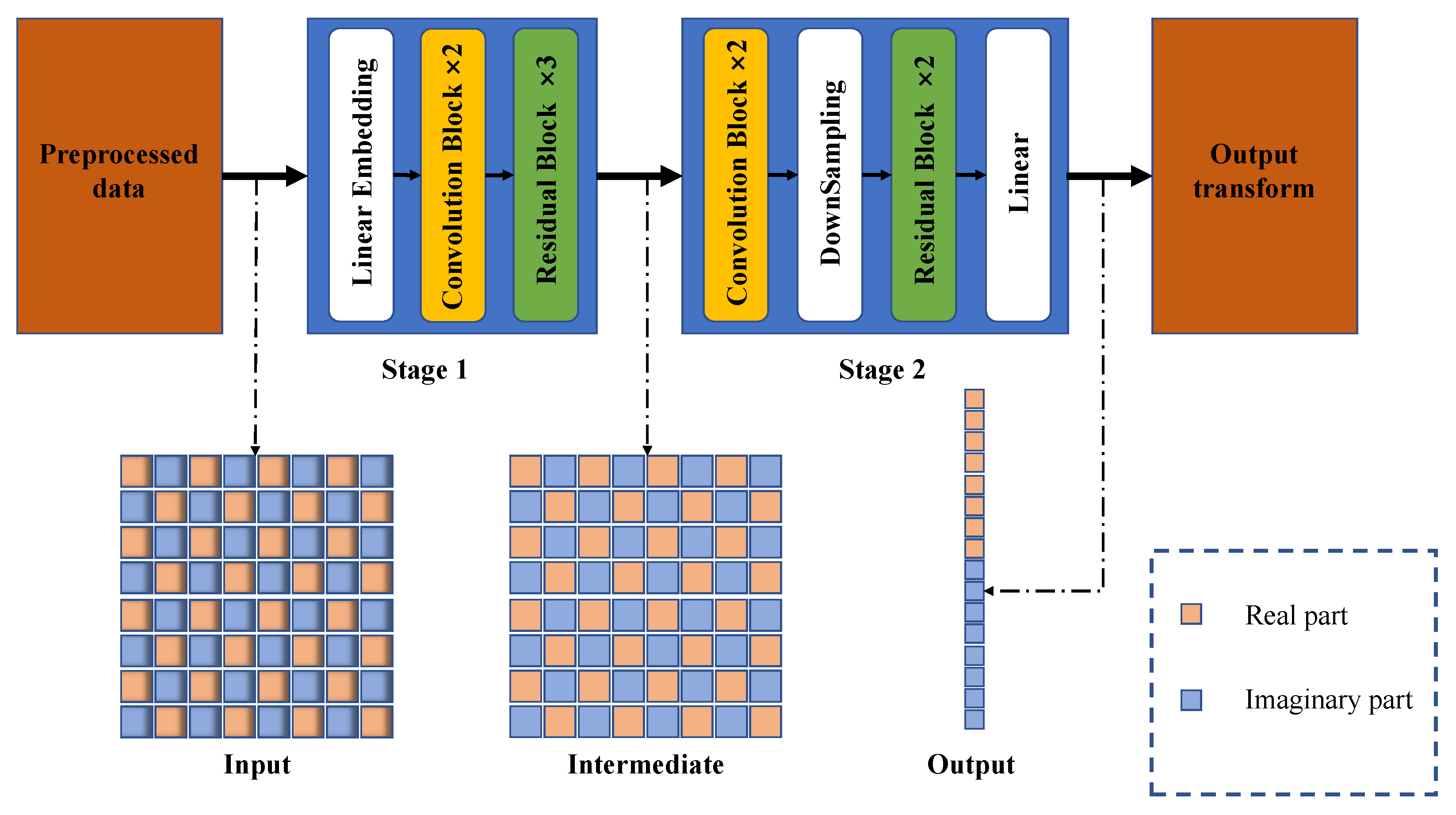
• Our proposed two-stage network has a clear physical meaning. Specifically, stage 1 utilizes several conventional blocks and residual blocks to estimate the SCM accurately, while in stage 2, a similar structure with an additional downsampling layer and linear layer is employed to compute the MVDR weights.

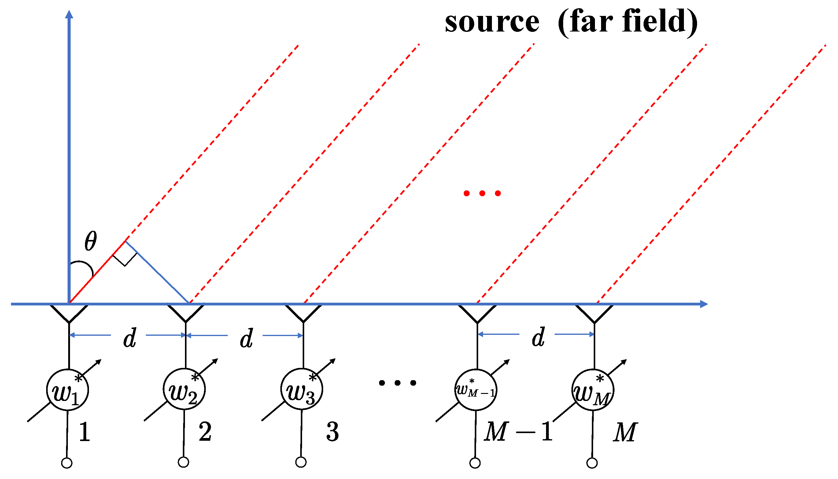
The remaining sections of this paper are structured as follows. Section 2 provides a problem formulation, while Section 3 presents detailed information on the proposed CNN architecture, data set, and training strategy. Numerical simulation results are presented in Section 4. Finally, Section 5 provides conclusions.

Notation: In this paper, vectors are denoted by boldface lowercase letters and matrices by boldface uppercase letters. The conjugate transpose, transpose, and inverse of a matrix are denoted by ${(·)}^{\mathrm{H}}$, ${(·)}^{\mathrm{T}}$, and ${(·)}^{-1}$, respectively. Additionally, $\mathrm{Tr}(·)$ and $\mathrm{diag}[·]$ represent the trace of a matrix and the diagonal matrix, respectively. The $l_2$-norm and Frobenius norm of a vector and matrix are denoted by $∥·∥$ and ${∥·∥}_{\mathrm{F}}$, respectively. The real and imaginary parts of a complex number are represented by $\mathrm{real}(·)$ and $\mathrm{imag}(·)$, respectively. We use $\mathrm{rand}[·]$ and $\mathrm{rand}(·)$ to denote discrete and continuous random sampling, respectively.

2. MVDR Estimator

In this paper, we consider a uniform linear array (ULA) consisting of M elements, as depicted in Figure 1. The array receives N snapshot data, where each snapshot contains the SoI and multiple SoAs. Moreover, we take into account the G/P errors, which are expressed as an error matrix $\mathsf{\Gamma }$. The received signal model can be expressed as

$$\mathbf{x}\left(n\right)=\mathsf{\Gamma }\mathbf{A}{\mathit{x}}_J\left(n\right)+\mathsf{\Gamma }{\mathit{a}}_0{x}_s\left(n\right)+{\mathit{x}}_n$$

(1)

here, $n=1,2,...,N$ represents the discrete time index. The vector ${\mathit{x}}_J={[x_{J1},x_{J1},...,x_{JL}]}^{\mathrm{T}}$ denotes the complex envelopes of L interferences, and ${\mathit{x}}_n$ represents the Gaussian white noise vector. The complex envelope of the SoI and its corresponding array steering vector ${\mathit{a}}_0$ are denoted by $x_s$ and $\mathbf{A}$, respectively. The matrix $\mathsf{\Gamma }\mathbf{A}$ is the array manifold matrix, where $\mathsf{\Gamma }$ corresponds to the G/P error matrix, and $\mathbf{A}$ contains the steering vectors for different angles of arrival (AoAs). The G/P error matrix $\mathsf{\Gamma }$ is given by the following formula:

$$\mathsf{\Gamma }=\mathrm{diag}[r_1{r}_2...r_N]$$

(2)

where

$$r_i=(1+A_i)e^{j{\varphi }_i},$$

(3)

and $A_i$ and ${\varphi }_i$ represent the gain and phase errors, respectively. Finally, we express the AoAs using the following notation:

$$\mathbf{A}=\left(\begin{array}{cccc}1& 1& \cdots & 1\\ e^{-j\beta sin{\theta }_{J1}}& e^{-j\beta sin{\theta }_{J2}}& \cdots & e^{-j\beta sin{\theta }_{JL}}\\ ⋮& ⋮& \ddots & ⋮\\ e^{-j\beta \left(M-1\right)sin{\theta }_{J1}}& e^{-j\beta \left(M-1\right)sin{\theta }_{J2}}& \cdots & e^{-j\beta \left(M-1\right)sin{\theta }_{JL}}\end{array}\right),\beta =\frac{2\pi d}{\lambda }$$

(4)

where ${\theta }_{Jl}$ represents the AoA of the $l^{th}$ SoA, d is the distance between the adjacent array elements, and $\lambda$ is the wavelength of the received signal.

The MVDR algorithm computes the array weight vector by minimizing the array output power subject to the constraint that the SoI is passed without distortion. The optimization problem can be expressed mathematically as

$$\left\{\begin{array}{c}{\displaystyle \underset{\mathit{w}}{min}}{\mathit{w}}^{\mathrm{H}}\mathbf{R}\mathit{w}\hfill \\ s.t.{\mathit{w}}^{\mathrm{H}}{\mathit{a}}_0=1\hfill \end{array}\right.$$

(5)

here, $\mathit{w}$ is the complex-valued weight vector, and $\mathbf{R}$ denotes the known covariance matrix of the array output vector. The solution to the optimization problem is given by

$$\mathit{w}=\frac{{\mathbf{R}}^{-1}{\mathit{a}}_0}{{\mathit{a}}_0^{\mathrm{H}}{\mathbf{R}}^{-1}{\mathit{a}}_0}.$$

(6)

This algorithm ensures that the array output is steered towards the SoI by minimizing the power of the interference and noise signals. The MVDR algorithm can effectively suppress the interferences for far-field sources, where the number of interferences is less than the array aperture.

As obtaining the exact covariance matrix $\mathbf{R}$ can be challenging in practical settings, the SCM $\widehat{\mathbf{R}}$ is typically used instead, which can be expressed as

$$\widehat{\mathbf{R}}=\frac{1}{N}\sum _{n=1}^N\mathit{y}{\left(n\right)}^{\mathrm{H}}\mathit{y}\left(n\right)$$

(7)

where

$$\mathit{y}\left(n\right)=\mathsf{\Gamma }\mathbf{A}{\mathit{x}}_J\left(n\right)+{\mathit{x}}_n\left(n\right)$$

(8)

denotes the noise-plus-interference vector and is employed to compute the SCM based on a finite observation frame of length N.

Furthermore, it is important to note that a mismatch may exist between the true steering vectors ${\mathit{a}}_0$ and the assumed steering vectors $\mathit{a}$. In such cases, the weight vector of the MVDR method, which utilizes the SCM and $\mathit{a}$, can be expressed as

$${\widehat{\mathit{w}}}_{\mathrm{MVDR}}=\frac{{\widehat{\mathbf{R}}}^{-1}\mathit{a}}{{\mathit{a}}^{\mathrm{H}}{\widehat{\mathbf{R}}}^{-1}\mathit{a}}.$$

(9)

In practical scenarios, where the number of snapshots is limited, the performance of the MVDR method can deteriorate substantially even when the steering vector for the SoI is accurately known [32]. Additionally, the mismatch between the true steering vector ${\mathit{a}}_0$ and the assumed steering vector $\mathit{a}$ can significantly impact the performance of MVDR. The SINR is used to evaluate the MVDR method’s performance, which can be formulated as

$$\mathrm{SINR}=\frac{{\widehat{\sigma }}_0^2{\widehat{\mathit{w}}}_{\mathrm{MVDR}}^{\mathrm{H}}{\mathit{a}}_0{\mathit{a}}_0^{\mathrm{H}}{\widehat{\mathit{w}}}_{\mathrm{MVDR}}}{{\widehat{\mathit{w}}}_{\mathrm{MVDR}}^{\mathrm{H}}\mathbf{Q}{\widehat{\mathit{w}}}_{\mathrm{MVDR}}}$$

(10)

where

$${\widehat{\sigma }}_0^2=\frac{1}{{\mathit{a}}^{\mathrm{H}}{\widehat{\mathbf{R}}}^{-1}\mathit{a}}$$

(11)

and $\mathbf{Q}$ denote the power of the SOI and the true interference-plus-noise covariance matrix, respectively. As N increases, the value of the output SINR will approach the optimal one, which is defined as

$${\mathrm{SINR}}_{\mathrm{opt}}={\widehat{\sigma }}_0^2{\mathit{a}}_0^{\mathrm{H}}{\mathbf{Q}}^{-1}{\mathit{a}}_0.$$

(12)

3. A Deep Neural Network for Robust Adaptive Beamforming

3.1. Architecture

DL-based array signal processing is data-driven, and it does not depend on prior assumptions about the array geometry or precisely estimated SCM [33]. In this study, an RBF method based on data-driven principles is expected to possess inherent adaptability to usual G/P errors as well as finite snapshot scenarios.

The proposed CNN-based model comprises an SCM estimator and an adaptive weight calculator, as shown in Figure 2. Leveraging the Hermitian property of the SCM, we transform it into a real-valued matrix, which preserves all the information. To this end, each element of the SCM is operated to obtain a corresponding element of the real-valued matrix, expressed as

$${\tilde{\mathbf{R}}}_{i,j}=\left\{\begin{array}{c}real\left({\widehat{\mathbf{R}}}_{i,j}\right)\hfill \\ imag\left({\widehat{\mathbf{R}}}_{i,j}\right)\hfill \end{array}\right.,\mathrm{for}i,j\in \{1,2,...,M\}$$

(13)

where ${\widehat{\mathbf{R}}}_{i,j}$ represents an element of the SCM and the subscripts i and j denote its row and column, respectively. Notably, there exist duplicate blocks in the proposed CNN-based model, specifically, the convolution block and residual block. The composition of these two blocks is illustrated in Figure 3. The convolution block includes a convolutional layer employing a convolution kernel of $(3\times 3)$, a batch normalization layer, and a ReLU activation function layer. The residual block is designed to address the issue of vanishing or exploding gradients and enhance the network performance [34]. To enable this, a residual connection is added to the convolution block. The convolution block and residual block are mathematically expressed as follows:

$${\mathit{c}}_{\mathrm{o}}=\mathrm{ReLU}({\mathbf{W}}^k \times \mathit{c}+{\mathit{b}}^k)$$

(14)

$${\mathit{r}}_{\mathrm{o}}=\mathrm{ReLU}({\mathbf{W}}^k \times \mathit{r}+{\mathit{b}}^k)+\mathit{r}$$

(15)

where ${\mathbf{W}}^k$ and ${\mathit{b}}^k$ are the convolution kernel and bias of the kth layer, respectively. ${\mathit{c}}_o$, $\mathit{c}$, ${\mathit{r}}_o$, and $\mathit{r}$ represent the output of the convolution block, the input of the convolution block, the output of the residual block, and the input of the residual block, respectively.

Stage 1 is primarily a data-driven estimator that forms the backbone of most RBF algorithms and has a significant impact on the proposed network’s performance. Given this, downsampling layers are not included in stage 1, thereby ensuring a larger feature map. Alternatively, stage 2 contains a downsampling layer to avoid making the network overly redundant.

Table 1. The Parameter Settings of Stage 1.

Type	Parameter
Input	(16,16)
Convolution block	4
Convolution block	16
Residual block	16
Residual block	16
Residual block	16
Output	(16,16)

and

Table 2. The Parameter Settings of Stage 2.

Type	Parameter
Input	(16,16)
Convolution block	4
Convolution block	16
DownSampling	(2,2)
Residual block	16
Residual block	16
Linear	1024
Output	(32,1)

depict the parameter settings of stage 1 and stage 2, respectively, in our proposed network. It should be noted that the tables are arranged in a top-to-bottom order to represent the connection order of each block in stage 1 and stage 2. The meaning of the parameters specified in Table 1 and Table 2 is as

• Input layer and Output layer: The data size of the input and output layers.
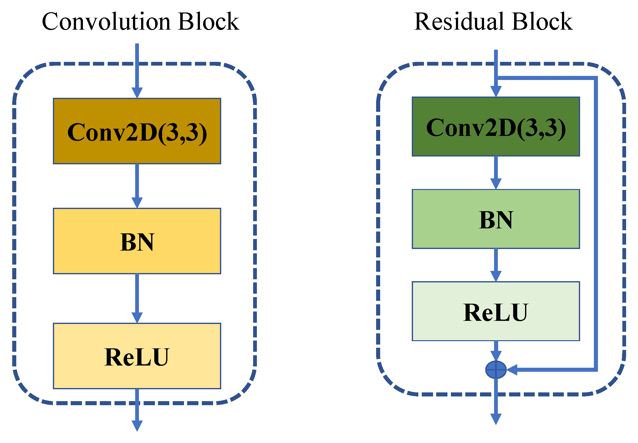
• Convolution block: The number of channels used in the convolution block.
• Residual block: The number of channels used in the residual block.
• Linear layer: The number of channels used in the linear layer.
• Downsampling layer: The downsampling size used in the Downsampling layer.

Here, the left column presents the layer name, while the right column provides a brief explanation of each associated parameter.

3.2. Dataset and Training

The proposed network uses simulated datasets, and a ULA with a half-wavelength element spacing is employed. The primary simulation conditions are listed in

Table 3. Simulation Conditions.

Parameter	Value
Num_array	$M=16$
snapshots	$N=4$
SOI	$\mathrm{rand}{[-40:1:40]}^{\circ }$
SNR	0 dB
SOAs	$\mathrm{rand}{[-70:1:70]}^{\circ }$
INR	$\mathrm{rand}[30:1:35]$ dB
G/P error maximum variance	${\sigma }_{r\_max}^2$ = $\mathrm{rand}(0:0.05)$

. To simulate scenarios with strong interference, the signal-to-noise ratio (SNR) is set to 0 dB, while the interference-to-noise ratio (INR) varies randomly between 30 and 35. Equation (3) is used to define the G/P error, with a constraint imposed on the range of $A_i\in [0,{\sigma }_r^2]$ and ${\varphi }_i\in {\sigma }_r^2\times [-\pi ,\pi ]$. Here, ${\sigma }_r^2$ is the G/P error variance ranging from 0 to ${\sigma }_{r\_max}^2$, which is the upper bound.

The proposed network undergoes a two-stage training process that involves separate pre-training stages using unique datasets, followed by fine-tuning as an end-to-end model. Two primary benefits of this approach include: Firstly, the two-stage training process enhances the neural network’s connection to the actual physical context by reinforcing its learned features, which increases its ability to capture the relevant information for the beamforming task. Secondly, the fine-tuning stage enhances the network’s stability, thereby enabling more efficient optimization and convergence, which results in improved performance on the target task.

To implement the proposed two-stage training process, we begin by pre-training the network stages separately using a large-scale dataset consisting of $4\times {10}^5$ records. Following this, we fine-tune the pre-trained network on downstream tasks using a smaller dataset comprising $5\times {10}^4$ records. Before inputting the data into the network, we normalize and convert it to real-valued format. The network output is represented as a label $\overline{\mathit{w}}$, which is defined by the equation:

$$\overline{\mathit{w}}={[\mathrm{real}\left({\mathit{w}}^T\right),\mathrm{imag}\left({\mathit{w}}^T\right)]}^T,$$

(16)

where $\mathit{w}$ is the weight vector. This formulation enables the calibration of the beamformer via a gradient descent optimization algorithm.

The network’s input comprises a real-valued SCM, denoted by $\tilde{\mathbf{R}}$, which is estimated using finite snapshots. The input undergoes two stages of processing. In stage 1, the network maps $\tilde{\mathbf{R}}$ to an intermediate output, $\overline{\mathbf{R}}$. In stage 2, $\overline{\mathbf{R}}$ is further processed and mapped to a linear output, $\tilde{\mathit{w}}$. The primary objective of the network is to minimize the loss between the output $\tilde{\mathit{w}}$ and the label $\overline{\mathit{w}}$ on the downstream tasks. Towards this goal, we define the loss function as follows:

$$\mathrm{loss}\triangleq \frac{1}{2}{∥\tilde{\mathit{w}}-\overline{\mathit{w}}∥}^2.$$

(17)

The aim of minimizing the loss function is to obtain accurate and stable beamforming weights that accurately capture the desired signal while suppressing interference and noise.

The training process for the network is formulated as an optimization problem, as shown below:

$${\left\{{\widehat{\mathbf{W}}}^k,{\widehat{\mathit{b}}}^k\right\}}_{k=1}^K=\underset{{\left\{{\mathbf{W}}^k,{\mathit{b}}^k\right\}}_{k=1}^K}{arg\min }\mathrm{loss}.$$

(18)

Once training is complete, the network can be used to predict adaptive weights $\widehat{\mathit{w}}$ corresponding to a new SCM $\widehat{\mathbf{R}}$. The adaptive weights can be obtained as follows:

$${\widehat{\mathit{w}}}^t={\tilde{\mathit{w}}}^t+i ✱ {\tilde{\mathit{w}}}^{t+M},t=1,2,...,M,$$

(19)

where t denotes the position of the element in the vector, and i is the imaginary unit.

The proposed method aims to achieve accurate and reliable beamforming while mitigating the adverse effects of interference and noise. By training the network on large-scale datasets and fine-tuning on downstream tasks, we can obtain highly optimized beamforming weight vectors that can be used in real-world scenarios.

4. Experiments

In this section, we assess the performance of the proposed CNN method through numerical simulations. We implement our method using TensorFlow and train the network using an NVIDIA GeForce RTX 3070 GPU and an Intel(R) Core(TM) i7-11700K CPU. We conduct several experiments to evaluate our method’s performance. In Experiment 1, we study the network convergence performance. In Experiments 2–4, we compare the performance of the oracle approximating shrinkage (OAS), the general linear combination (GLC), and our proposed method. We note that we do not compare our method with existing DL-beamformers for the following reasons:

• In [27], the output of the network is an ultrasound image obtained after adaptive processing, which can be essentially regarded as a spectral estimator. This differs from our CNN beamformer’s output, which is a set of adaptive weights.
• In [29], the DoA of the signal must be known a priori, which is not required in our CNN beamformer.
• In [30], the 1D CVCNN RBF method uses much larger training samples (100 to 400 snapshots) compared to our proposed method, which only requires four snapshots or fewer.

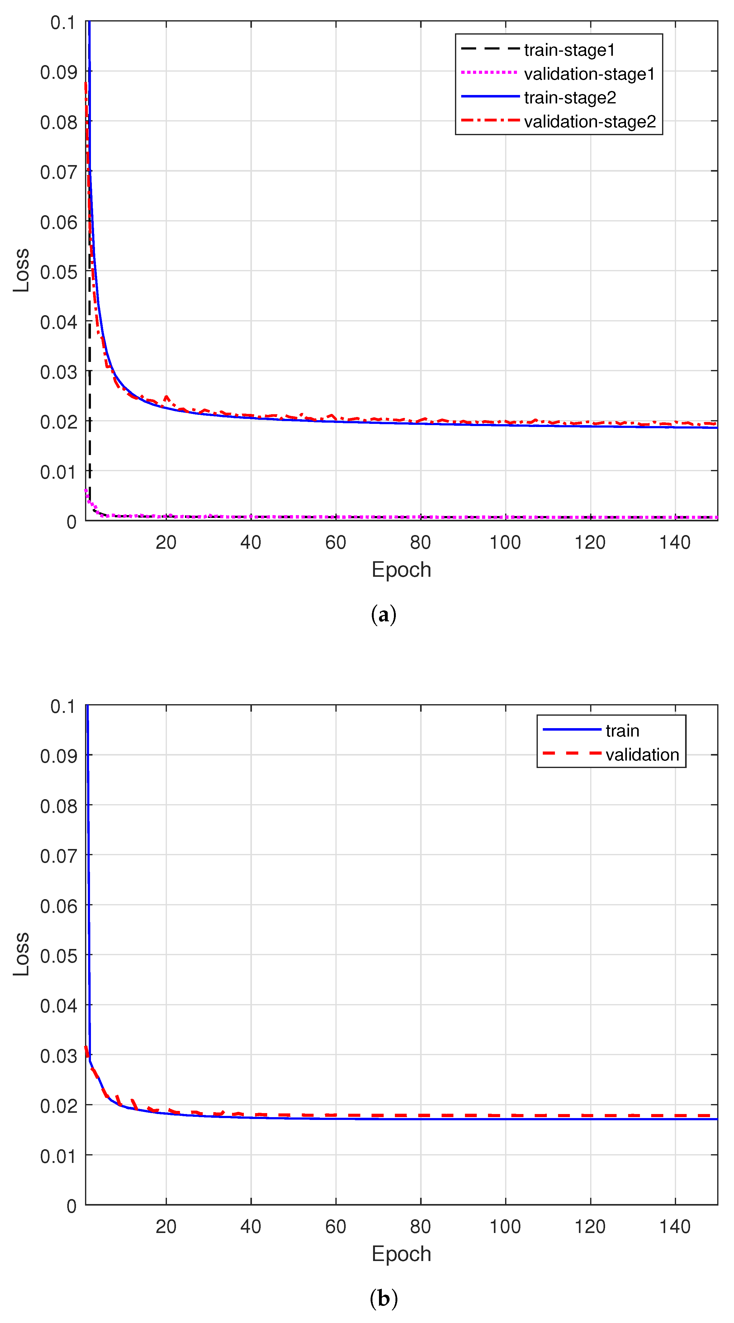
4.1. Network Convergence Performance

We utilize stochastic gradient descent [35] during training to update the network’s parameters. To dynamically compute the learning rate (LR), we employ the Adam optimization algorithm [36] with parameters ${\beta }_1=0.9$, ${\beta }_2=0.999$, and $\eta =1\times {10}^{-7}$. We also use a gradual warm-up method with 10 steps to gradually increase the LR. The initial LR and base LR are set to $2\times {10}^{-2}$ and $0.05$, respectively. Once the LR reaches the preset base LR, it decays exponentially with a decay rate of $1\times {10}^{-5}$ until the end of training. The training epoch is set to 150 by default.

Figure 4 shows the network convergence performance. Figure 4a,b present the mean squared error (MSE) loss per epoch for pre-training and fine-tuning, respectively. The figure indicates that the pre-training and fine-tuning stages converge quickly and do not exhibit signs of overfitting. Furthermore, the MSE loss of the whole network is further reduced after the fine-tuning stage.

Overall, our results demonstrate that our proposed approach can achieve high prediction accuracy while mitigating overfitting issues.

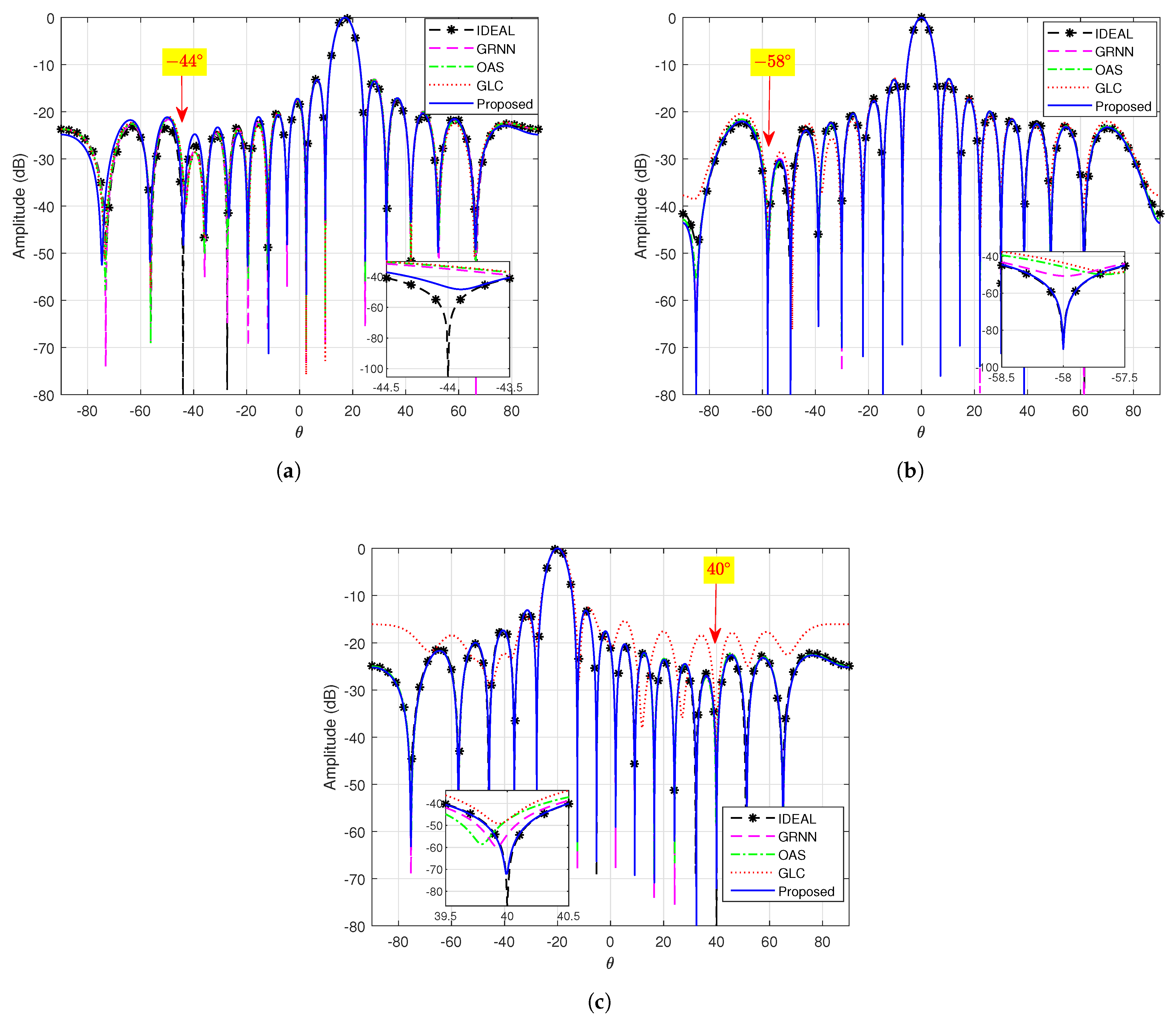
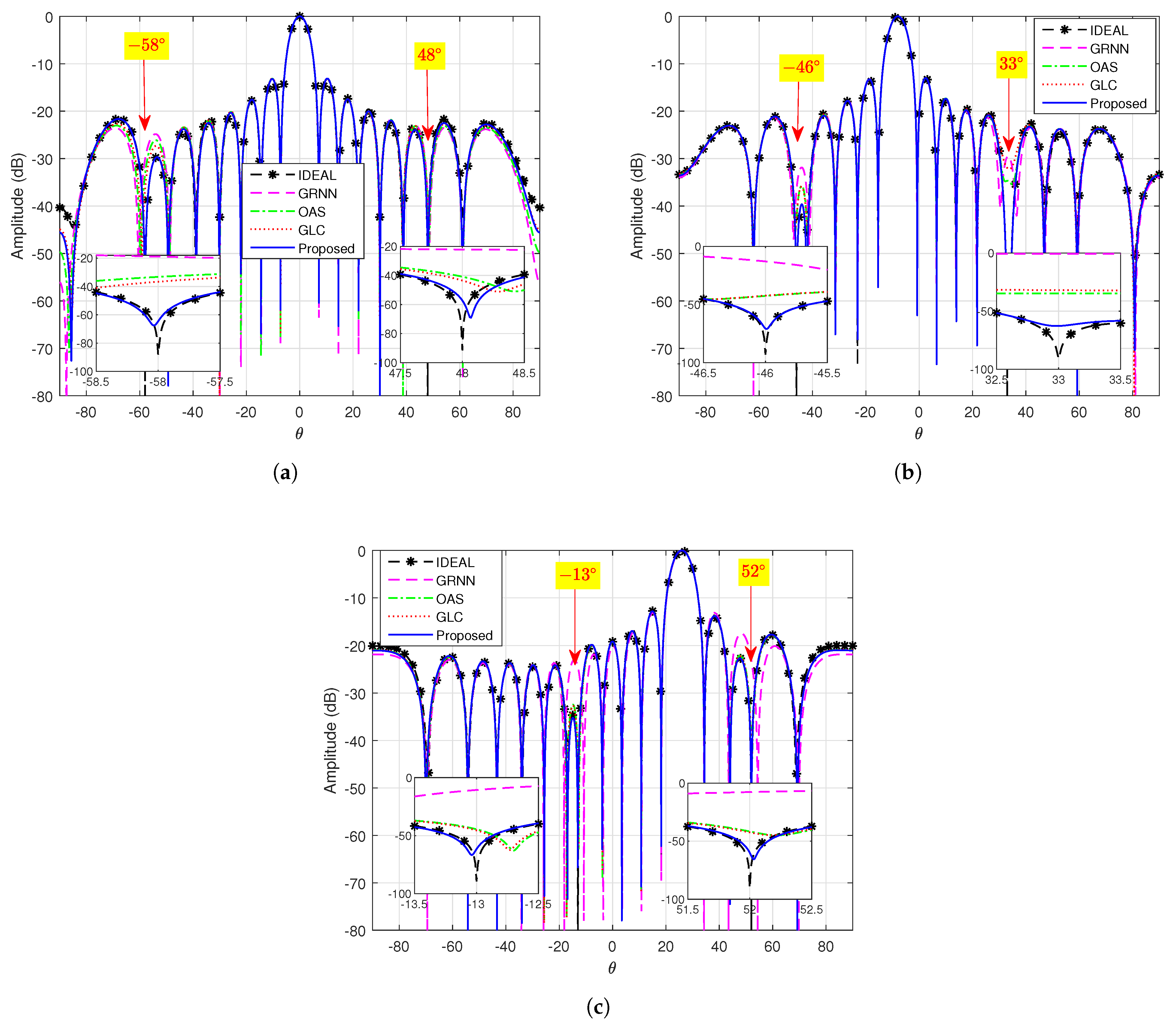
4.2. Adaptive Pattern Comparison in the Case of Finite Snapshots

To intuitively and fairly illustrate the performance of our proposed network, we use adaptive patterns. These patterns are generated using a fixed G/P error of zero to represent the performance in the absence of G/P errors. The number of snapshots used is set to 4, which is far less than the array element number. The pattern can be defined as follows:

$$P\left(\theta \right)={\mathit{w}}^{\mathrm{H}}\mathit{a}\left(\theta \right)$$

(20)

where $\mathit{a}\left(\theta \right)$ is the steering vector related to the azimuth angle $\theta$.

We generate adaptive patterns using GRNN [31], OAS [13], GLC [14], and CNN methods. The ideal adaptive pattern, calculated using the MVDR method with thirty thousand snapshots, gives the upper bound of performance. Figure 5 shows some typical examples in the presence of a single interference. To aid observation, we marked the interference position with red arrows on the pattern and partially enlarged the region near the interference. The GRNN, OAS, GLC, and CNN methods all form nulls in the locations of the interference without obvious distortion. Our proposed method achieves deeper notches than other methods (15 dB higher) with less positional offset. Figure 6 shows typical examples in the presence of double interferences. Interestingly, we note that the positional offset of OAS, GLC, and GRNN increases significantly with the increasing number of interferences, while our method still maintains stability.

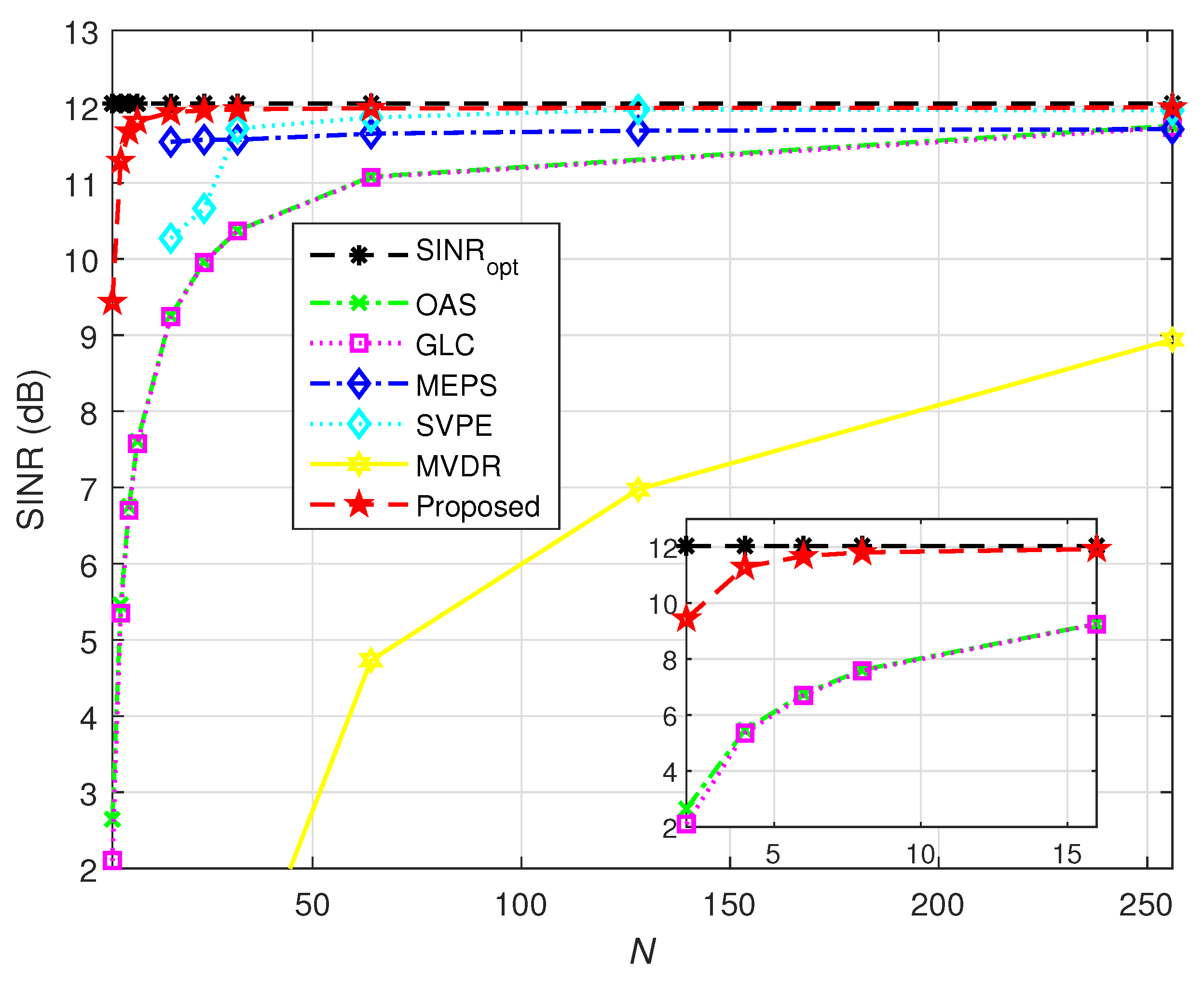
4.3. Performance Comparison of Convergence

We compare the convergence of different methods based on the output SINR. The optimal SINR (obtained using (10)) is included for reference. For this scenario, the SNR and INR are fixed to 0 dB and 30 dB, respectively. We perform 5000 Monte Carlo trials. Figure 7 shows the beamformer output SINR versus the snapshot number N. The angular sector of the desired signal is set to ${\Theta }=\left[-6^{\circ },6^{\circ }\right]$, while the complement sector of ${\Theta }$ is $\overline{{\Theta }}=\left[-{90}^{\circ },-6^{\circ }\right)\cup \left(6^{\circ },{90}^{\circ }\right]$ for the beamformers of MEPS [18] and SVPE [19].

As MEPS, SVPE, and MVDR cannot work when N is less than M, the corresponding parts are excluded from Figure 7. Note that OAS and GLC methods can still work when $\widehat{\mathit{R}}$ is rank deficient $(N<M)$ but CNN significantly outperforms them. The output SINR of GLC and OAS methods gradually approaches that of the proposed CNN method with increasing N. Furthermore, even when $N>M$, our proposed method achieves output SINR closer to the optimal SINR than the other comparison methods.

4.4. Performance Comparison in the Presence of G/P Errors

Table 4. Performance in the Presence of Different G/P Errors.

G/P Errors	SINR (dB)
	OPT	GLC	OAS	Proposed
0.000	12.0327	5.4625	5.5570	11.3433
0.005	12.0325	5.3563	5.4843	10.8617
0.010	12.0321	5.2422	5.3666	9.8965
0.015	12.0321	5.3172	5.4270	8.8833
0.020	12.0324	5.3730	5.4808	8.0496
0.025	12.0322	5.3916	5.4918	7.3809
0.030	12.0320	5.3638	5.4664	6.9473
0.035	12.0316	5.3609	5.4643	6.5472
0.040	12.0315	5.3320	5.4362	6.2157
0.045	12.0303	5.3125	5.4056	5.8945
0.050	12.0299	5.3886	5.4646	5.5795

shows the average output SINR of the OPT, GLC, OAS, and our proposed CNN methods in the presence of different G/P errors. For this scenario, SNR and INR are fixed at 0 dB and 30 dB, respectively. The G/P errors are increased from 0 to 0.05 in steps of 0.005, and 5000 Monte Carlo trials are performed at each step. Note that the G/P error typically does not exceed 0.05 in practical applications.

The results suggest that the performance of the CNN method is close to the upper bound and significantly better than OAS and GLC methods when the G/P error is minor. Although the GLC and OAS algorithms can exhibit certain robustness when the G/P error changes, there is still a performance gap compared to the OPT. Furthermore, although the SINR of the CNN method gradually decreases with increasing G/P errors, it remains superior to the OAS and GLC methods. Overall, our proposed method provides an average SINR gain of 3–5 dB in the presence of G/P errors compared to the OAS and GLC methods.

4.5. Computational Complexity Comparison

DL requires considerable time during network training, which may hinder its implementation in real-time applications. However, the proposed approach in this work overcomes this issue by conducting the training offline. After the network is trained, online computations only entail basic matrix and vector operations such as multiplication and addition. Additionally, the computational complexity of the proposed approach based on CNN can be accurately formulated by

$$O\left(\sum _{k=1}^K{f}_k^3{\left(M-f_k+1\right)}^2{n}_k\right)$$

(21)

where K represents the number of layers in the CNN network, $f_k$ represents the dimension of the convolution kernel in the k-th layer, and $n_k$ represents the number of convolution kernels in the k-th layer of the network. By substituting the network parameters set in this article into (21), the computational complexity of the proposed method can be obtained.

Table 5. Analysis of Computational Complexity and Running Time.

Method	Computational Complexity	Running Time (s)
Proposed	$O\left(2808M^2\right)$	0.0118
OAS	$O(2M^3+N{M}^2+5M^2)$	0.0025
GLC	$O(M^3+3N{M}^2+N^{2}M+2N^2)$	0.0017

presents a comprehensive comparison of the computational complexity and online running time of OAS, GLC, and the proposed method. Notably, the online running time was calculated using $M=16,N=4$, and the average of 1000 runs to minimize the influence of any potential randomness. As demonstrated in the table, the computational complexity of the CNN method is of the order of $M^2$, while OAS and GLC algorithms’ computational complexity is of the order of $M^3$. However, it should be acknowledged that OAS and GLC algorithms can complete computations swiftly when M is small. Although the CNN algorithm’s online running time is slightly longer than that of the OAS and GLC algorithms, it is still within the realistic time requirements for practical applications.

5. Conclusions

In this paper, we propose a new method for generating adaptive weights for beamforming. We build a factored network where the two stages are pre-trained separately with different datasets and then fine-tuned as an end-to-end network. Our CNN-based RBF approach is data-driven, which does not require prior model parameters such as array manifold and accurate SCM, making it advantageous for obtaining robust performance in the presence of G/P errors and finite snapshots.

We compare the proposed method with classical techniques in terms of performance. Simulation results demonstrate that our proposed CNN method outperforms OAS and GLC methods under non-ideal conditions such as small N or in the presence of G/P errors. In conclusion, the proposed approach offers a promising alternative for beamforming that can drastically improve its accuracy and robustness.

References

1. Bryn, F. Optimum signal processing of three-dimensional arrays operating on Gaussian signals and noise. Acoust. Soc. Am. 1962, 34, 289–297. [Google Scholar] [CrossRef]
2. Applebaum, S. Adaptive arrays. IEEE Trans. Antennas Propag. 1976, 24, 585–598. [Google Scholar] [CrossRef]
3. Green, P.E., Jr.; Kelly, E.J., Jr.; Levin, M.J. A comparison of seismic array processing methods. Geophys. J. Int. 1966, 11, 67–84. [Google Scholar] [CrossRef] [Green Version]
4. Choi, S.; Shim, D. A novel adaptive beamforming algorithm for a smart antenna system in a CDMA mobile communication environment. IEEE Trans. Veh. Technol. 2000, 49, 1793–1806. [Google Scholar] [CrossRef] [Green Version]
5. Navarro-Camba, E.A.; Felici-Castell, S.; Segura-García, J.; García-Pineda, M.; Pérez-Solano, J.J. Feasibility of a Stochastic Collaborative Beamforming for Long Range Communications in Wireless Sensor Networks. Electronics 2018, 7, 417. [Google Scholar] [CrossRef] [Green Version]
6. Capon, J. High-resolution frequency-wave number spectrum analysis. Proc. IEEE 1969, 57, 1408–1418. [Google Scholar] [CrossRef] [Green Version]
7. Shahbazpanahi, S.; Gershman, A.B.; Luo, Z.Q.; Wong, K.M. Robust adaptive beamforming for general-rank signal models. IEEE Trans. Signal Process. 2003, 51, 2257–2269. [Google Scholar] [CrossRef]
8. Cox, H.; Zeskind, R.; Owen, M. Robust adaptive beamforming. IEEE Trans. Acoust. Speech Signal Process. 1987, 35, 1365–1376. [Google Scholar] [CrossRef] [Green Version]
9. Feldman, D.D.; Griffiths, L.J. A projection approach for robust adaptive beamforming. IEEE Trans. Signal Process. 1994, 42, 867–876. [Google Scholar] [CrossRef]
10. Lee, C.C.; Lee, J.H. Eigenspace-based adaptive array beamforming with robust capabilities. IEEE Trans. Antennas Propag. 1997, 45, 1711–1716. [Google Scholar]
11. Vorobyov, S.A.; Gershman, A.B.; Luo, Z.Q. Robust adaptive beamforming using worst-case performance optimization: A solution to the signal mismatch problem. IEEE Trans. Signal Process. 2003, 51, 313–324. [Google Scholar] [CrossRef] [Green Version]
12. Ledoit, O.; Wolf, M. Improved estimation of the covariance matrix of stock returns with an application to portfolio selection. J. Empir Finance 2003, 10, 603–621. [Google Scholar] [CrossRef] [Green Version]
13. Chen, Y.; Wiesel, A.; Eldar, Y.C. Shrinkage algorithms for MMSE covariance estimation. IEEE Trans. Signal Process. 2010, 58, 5016–5029. [Google Scholar] [CrossRef] [Green Version]
14. Du, L.; Li, J.; Stoica, P. Fully automatic computation of diagonal loading levels for robust adaptive beamforming. IEEE Trans. Aerosp. Electron. Syst. 2010, 46, 449–458. [Google Scholar] [CrossRef]
15. Wu, R.; Bao, Z.; Ma, Y. Control of peak sidelobe level in adaptive arrays. IEEE Trans. Antennas Propag. 1996, 44, 1341–1347. [Google Scholar]
16. Gu, Y.; Leshem, A. Robust Adaptive Beamforming Based on Interference Covariance Matrix Reconstruction and Steering Vector Estimation. IEEE Trans. Signal Process. 2012, 60, 3881–3885. [Google Scholar]
17. Mohammadzadeh, S.; Kukrer, O. Adaptive beamforming based on theoretical interference-plus-noise covariance and direction-of-arrival estimation. IET Signal Process. 2018, 12, 819–825. [Google Scholar] [CrossRef]
18. Mohammadzadeh, S.; Nascimento, V.H.; De Lamare, R.C.; Kukrer, O. Maximum Entropy-Based Interference-Plus-Noise Covariance Matrix Reconstruction for Robust Adaptive Beamforming. IEEE Signal Process. Lett. 2020, 27, 845–849. [Google Scholar] [CrossRef]
19. Zheng, Z.; Zheng, Y.; Wang, W.Q.; Zhang, H. Covariance Matrix Reconstruction With Interference Steering Vector and Power Estimation for Robust Adaptive Beamforming. IEEE Trans. Veh. Technol. 2018, 67, 8495–8503. [Google Scholar] [CrossRef]
20. Zhu, X.; Xu, X.; Ye, Z. Robust adaptive beamforming via subspace for interference covariance matrix reconstruction. Signal Process. 2020, 167, 107289. [Google Scholar] [CrossRef]
21. Mohammadzadeh, S.; Nascimento, V.H.; De Lamare, R.C.; Kukrer, O. Robust adaptive beamforming based on virtual sensors using low-complexity spatial sampling. Signal Process. 2021, 188, 108172. [Google Scholar] [CrossRef]
22. Davoli, A.; Guerzoni, G.; Vitetta, G.M. Machine learning and deep learning techniques for colocated MIMO radars: A tutorial overview. IEEE Access 2021, 9, 33704–33755. [Google Scholar] [CrossRef]
23. Pan, P.; Zhang, Y.; Deng, Z.; Qi, W. Deep learning-based 2-D frequency estimation of multiple sinusoidals. IEEE Trans. Neural Networks Learn. Syst. 2022, 33, 5429–5440. [Google Scholar] [CrossRef]
24. Duan, K.; Chen, H.; Xie, W.; Wang, Y. Deep learning for high-resolution estimation of clutter angle-Doppler spectrum in STAP. IET Radar Sonar Navig. 2022, 16, 193–207. [Google Scholar] [CrossRef]
25. Rogers, J.; Ball, J.E.; Gurbuz, A.C. Estimating the Number of Sources via Deep Learning. In Proceedings of the 2019 IEEE Radar Conference (RadarConf), Boston, MA, USA, 22–26 April 2019; pp. 1–5. [Google Scholar]
26. Bianco, S.; Napoletano, P.; Raimondi, A.; Feo, M.; Petraglia, G.; Vinetti, P. AESA Adaptive Beamforming Using Deep Learning. In Proceedings of the 2020 IEEE Radar Conference (RadarConf20), Florence, Italy, 21–25 September 2020; pp. 1–6. [Google Scholar]
27. Luijten, B.; Cohen, R.; de Bruijn, F.J.; Schmeitz, H.A.; Mischi, M.; Eldar, Y.C.; van Sloun, R.J. Adaptive ultrasound beamforming using deep learning. IEEE Trans. Med. Imaging 2020, 39, 3967–3978. [Google Scholar] [CrossRef] [PubMed]
28. Hamza, S.A.; Amin, M.G. Learning Sparse Array Capon Beamformer Design Using Deep Learning Approach. In Proceedings of the 2020 IEEE Radar Conference (RadarConf20), Florence, Italy, 21–25 September 2020. [Google Scholar]
29. Mallioras, I.; Zaharis, Z.D.; Lazaridis, P.I.; Pantelopoulos, S. A novel realistic approach of adaptive beamforming based on deep neural networks. IEEE Trans. Antennas Propag. 2022, 70, 8833–8848. [Google Scholar] [CrossRef]
30. Mohammadzadeh, S.; Nascimento, V.H.; De Lamare, R.C.; Hajarolasvadi, N. Robust Beamforming Based on Complex-Valued Convolutional Neural Networks for Sensor Arrays. IEEE Signal Process. Lett. 2022, 29, 2108–2112. [Google Scholar] [CrossRef]
31. Xiao, X.; Lu, Y. Data-Based Model for Wide Nulling Problem in Adaptive Digital Beamforming Antenna Array. IEEE Antennas Wirel. Propag. Lett. 2019, 18, 2249–2253. [Google Scholar] [CrossRef]
32. Carlson, B.D. Covariance matrix estimation errors and diagonal loading in adaptive arrays. IEEE Trans. Aerosp. Electron. Syst. 1988, 24, 397–401. [Google Scholar] [CrossRef]
33. Liu, Z.M.; Zhang, C.; Philip, S.Y. Direction-of-arrival estimation based on deep neural networks with robustness to array imperfections. IEEE Trans. Antennas Propag. 2018, 66, 7315–7327. [Google Scholar] [CrossRef]
34. He, K.; Zhang, X.; Ren, S.; Sun, J. Deep Residual Learning for Image Recognition. In Proceedings of the IEEE Conference on Computer Vision and Pattern Recognition (CVPR), Las Vegas, NV, USA, 27–30 June 2016; pp. 770–778. [Google Scholar]
35. Amari, S.I. Backpropagation and stochastic gradient descent method. IEEE Trans. Antennas Propag. 1993, 5, 185–196. [Google Scholar] [CrossRef]
36. Kingma, D.P.; Ba, J. Adam: A Method for Stochastic Optimization. In Proceedings of the International Conference on Learning Representations (ICLR), San Diego, CA, USA, 7–9 May 2015. [Google Scholar]
Figure 1. Diagram of ULA.
Electronics 12 02751 g001
Figure 2. Overview of the proposed model.
Electronics 12 02751 g002
Figure 3. Blocks.
Electronics 12 02751 g003
Figure 4. Assessing the Network Convergence Performance. (a) MSE loss per epoch of stage 1 and stage 2 during pre-training. (b) MSE loss per epoch during fine-tuning.
Electronics 12 02751 g004
Figure 5. Single interference performance comparison in the absence of G/P errors. The desired signal positions of (ac) are 17°, 0°, and −20°, respectively. The interference positions of (ac) are 21°, −54°, and −46°, respectively. The INR of used interference in (ac) are 30 dB, 31 dB, and 34 dB, respectively.
Electronics 12 02751 g005
Figure 6. Double interference performance comparison in the absence of G/P errors. The desired signal positions of (ac) are −8°, 0°, and 26°, respectively. The position and INR of used two interference in (a) are −14° & 33 dB and 15° & 33 dB; in (b) are −34° & 31 dB and 13° & 32 dB; in (c) are −61° & 35 dB and 10° & 30 dB.
Electronics 12 02751 g006
Figure 7. Performance comparison with different snapshots.
Electronics 12 02751 g007