Chaos Moth Flame Algorithm for Multi-Objective Dynamic Economic Dispatch Integrating with Plug-In Electric Vehicles

Abstract

Dynamic economic dispatch (DED) plays an important role in the operation and control of power systems. The integration of DED with space and time makes it a complex and challenging problem in optimal decision making. By connecting plug-in electric vehicles (PEVs) to the grid (V2G), the fluctuations in the grid can be mitigated, and the benefits of balancing peaks and filling valleys can be realized. However, the complexity of DED has increased with the emergence of the penetration of plug-in electric vehicles. This paper proposes a model that takes into account the day-ahead, hourly-based scheduling of power systems and the impact of PEVs. To solve the model, an improved chaos moth flame optimization algorithm (CMFO) is introduced. This algorithm has a faster convergence rate and better global optimization capabilities due to the incorporation of chaotic mapping. The feasibility of the proposed CMFO is validated through numerical experiments on benchmark functions and various generation units of different sizes. The results demonstrate the superiority of CMFO compared with other commonly used swarm intelligence algorithms.

1. Introduction

In the stage of power system planning and operation, economic dispatch (ED) plays a critical role in maintaining financial benefits due to the high value of fossil fuels used in power plants. A minor improvement in ED may result in significant cost savings. Moreover, it is imperative to address the problem of power grid fluctuations, as fluctuations in power generation can cause significant damage to electrical equipment and result in substantial economic losses. However, in practice, precisely modeling ED is difficult as it encompasses various factors such as the valve point effects and transmission losses, making it non-convex, non-smooth, non-linear, and non-differentiable. Therefore, evolutionary computation techniques are usually chosen to solve such problems, including genetic algorithms (GA), particle swarm optimization (PSO), ant colony optimization (ACO), and others.

Especially in recent years, many meta-heuristic algorithms have been applied to ED problems, including many new and improved algorithms that have gained some achievements. For example, the cogeneration is introduced into an ED problem that can achieve energy saving and improve environmental quality, which is solved by the cuckoo search algorithm (CSA) with penalty function. However, only low-dimensional cases have been studied, and experiments and analyses of high-dimensional cases are lacking [1]. A new parallel hybrid meta-heuristic method, combining the hybrid topology binary particle swarm optimization algorithm, adaptive differential evolution algorithm, and lambda iterative method, is proposed to solve the ED problem; however, no smart demand side management is achieved [2]. A chaotic local search-based bee optimization algorithm is utilized for the ED problem, which has the advantages of fast convergence and strong local search ability [3]. A short-term load ED problem combines the ED problem with machine learning-based short-term load forecasting (STLF), where a new energy dispatch model is proposed and solved by a new dynamic genetic algorithm; however, experiments were conducted on only three test systems and no other new energy generation methods were introduced [4]. Due to the uncertainty of wind power, the wind speed model is considered in the ED problem, which is conducive to exploring a more balanced low-carbon power dispatching strategy for wind power integrated systems, and is investigated by the flower pollination algorithm to solve this class of economic dispatching problems [5,6]. The chaotic map is utilized to improve the performance of the bat algorithm, which is presented to solve the static economic dispatch problem [7]. The cuckoo search algorithm (CSA) is applied to ED problems where wind turbines and fuel cells are considered, and a cuckoo search algorithm for microgrid power dispatch problems has also been proposed with some prospect [8]. The fuzzy dominance is used to select Pareto optimal front (POF) and the multi-objective fuzzy dominance-based bacterial foraging algorithm is proposed to solve the economic emission dispatch problem; however, it was not compared with other multi-objective algorithms, and it was difficult to reflect the superiority of the improved algorithm [9]. A multi-objective optimization algorithm based on time-varying accelerated particle swarm optimization has been introduced to the cogeneration problem with a high convergence rate and solving the uncertainty of energy demand and supply for intermittent renewable energy sources, but the method has only been applied to a 7-unit test system and there is a lack of research on other scale test systems [10]. Additionally, an improved large-scale symbiotic organism search algorithm has been proposed to address ED problems with valve point effects, demonstrating an increased ability to identify stable and high-quality solutions in a reasonable amount of time [11]. By combining stochastic exploratory search and learning strategies, an improved gray wolf optimization (GWO) algorithm is designed to solve the ED problem in different dimensions and effectively reduces the generation cost compared with other algorithms [12,13]. In order to consider the impact of wind power generation, a novel chaotic quantum genetic algorithm was developed to solve the ED problem of wind power generation with good results [14]. An improved competitive group optimization algorithm has been proposed to handle both static and dynamic ED problems and minimize the total fuel cost by determining the intra-regional generation and inter-regional power exchange, and has advantages in terms of solution accuracy and reliability compared with other algorithms [15]. Furthermore, an improved fireworks algorithm has been applied to multi-regional ED problems, featuring a new constraint-handling scheme that corrects potential solutions within the feasible search space [16,17]. To address multi-regional ED problems, a chaotic artificial bee colony algorithm has been introduced. This algorithm employs the modified sub-gradient method (MSG) to convert the constrained problem into an unconstrained one, and a resulting improved harmony search algorithm (HSA) has been designed for ED problems [18,19,20].

Economic dispatch includes static economic dispatch and dynamic economic dispatch. Static economic dispatch assumes constant load, which is difficult to adapt to the dynamic changes of actual power load. Dynamic economic dispatch generally divides a day into 24 h and optimizes daily economic dispatch according to daily load forecast, which is more in line with the actual power system operation. The mainstream of current research is dynamic economic dispatch. The integration of plug-in electric vehicles (PEVs) into DED problems has gained attention with the rise of new energy vehicles [21,22,23,24,25,26]. Connecting PEVs to the grid (V2G) can help mitigate the fluctuations of the grid and achieve peak clipping and valley filling. For large-scale PEVs, a distributed access and central management approach is generally adopted. The PEVs dispatching center can exchange energy and information directly with the power grid, and then the PEVs dispatching center directs the energy exchange of each vehicle according to the actual situation of the serviceable PEVs, so that orderly charging and discharging coordinated management can be realized. In addition, the conversion speed of PEVs charging and discharging is very fast, so it can be seen as a distributed energy storage device that can be charged and discharged, and the real-time power flow between PEVs and the grid can be realized through bi-directional power conversion technology, which is also known as electric vehicle to grid (V2G). By accurately transmitting information in both directions between the dispatch center and the PEVs, it is possible to achieve bi-directional, real-time, and controllable energy conversion. Of course, this involves the integration of various technologies such as power electronics, communication, power scheduling, and load forecasting. Therefore, it is possible to control the PEVs for orderly discharging when in the peak period of electricity consumption and control the PEVs for orderly charging when in the low peak period of electricity consumption, so as to reduce the burden of the power grid to a certain extent, improve the safety of the power grid, and achieve the purpose of coordinated charging and discharging.

Compared with the ordinary large-scale energy storage, the use of PEVs as a buffer for the grid is due to the fact that electricity can flow in both directions between the grid and PEVs. Moreover, as the number of PEVs increases, it is necessary to rationalize their management, otherwise the grid will be overloaded when the number of PEVs reaches a certain scale. Despite its potential benefits, the DED problem with PEVs has received limited attention in the literature. The moth flame optimization (MFO) algorithm was introduced by Seyedali Mirjalili in 2015 [27]. It is a swarm intelligence optimization algorithm inspired by the flight patterns of moths, and has been widely used for its simple structure, few parameters, and high efficiency. In recent years, various meta-heuristic algorithms, such as the dragonfly algorithm (DA) [28], multi-verse optimizer (MVO) [29], sine cosine algorithm (SCA) [30], ant line optimizer (ALO) [31], grasshopper optimization algorithm (GOA) [32], salp swarm algorithm (SSA) [33], whale optimization algorithm (WOA) [34], marine predator algorithm (MPA) [35], grey wolf optimizer (GWO) [36], binary bat algorithm (BBA) [37], teaching-learning based optimization (TLBO) [38], have been proposed and applied to the DED problem. However, the application of the MFO algorithm to solve the DED problem with PEVs remains limited.

The remainder of this paper is organized as follows. The DED problem integrating with PEVs formulation is presented in Section 2. The proposed CMFO algorithm is described in detail in Section 3. The performance of CMFO is validated on benchmark problems [39,40], as well as DED cases with PEVs in Section 4. The experimental results are analyzed in Section 5. Finally, the summary of the paper and future work directions are given in Section 6.

2. Problem Formulation

The target of DED integrating with PEVs is to determine the optimal generation levels of all online units and PEVs during a specified period of time [41,42], so as to minimize both the fuel cost of thermal power plants and grid fluctuation simultaneously for a given load demand while satisfying various constraints [43,44].

2.1. Objective Function

Considering that the steam valve of the steam turbine is suddenly open and it would have a certain impact on the energy consumption of the units, which is the so-called valve point loading effect, the objective function of total fuel cost is given by:

$$\min f_1(P)={\displaystyle \sum _{t=1}^T{\displaystyle \sum _{i=1}^N{a}_i+b_i{P}_{t,i}+c_i{P}_{t,i}^2}+|e_i\sin [f_i(P_i^{\min }-P_{t,i})]|}$$

(1)

where $f_1(P)$ is the total fuel cost of the thermal power units, $T$ is the number of periods in a scheduling cycle, $N$ is the total number of generator units, $a_i$, $b_i$, $c_i$, $e_i$ and $f_i$ are cost coefficients of $i\mathrm{t}\mathrm{h}$ the unit, $P_{t,i}$ is the output power of the $i\mathrm{t}\mathrm{h}$ unit at time t, and $P_i^{\min }$ is the minimum output power of the $i\mathrm{t}\mathrm{h}$ unit.

Furthermore, the large fluctuation in power generation could cause damaging impacts on the power grid. So, V2G is introduced to fill the valley and clip peak, which is formulated as:

$$\min f_2(P,P_{PEV})={\displaystyle \sum _{t=1}^T[{\displaystyle \sum _{i=1}^N(P_{t+1,i}+P_{PEV,t+1}-P_{L,t+1})-{\displaystyle \sum _{i=1}^N(P_{t,i}+P_{PEV,t}-P_{L,t})}}{]}^2}$$

(2)

where $f_2(P,P_{PEV})$ is to minimize grid fluctuations, $P_{PEV,t}$ is the exchange power between the electric vehicle and the grid at time t, and $P_{L,t}$ is transmission loss at time t.

Here, the objective functions $f_1$ and $f_2$ are combined into $f$ using a weighting factor $\omega$, which can be expressed by:

$$f=f_1+\omega f_2$$

(3)

2.2. Constraints

2.2.1. Power Capacity Constraint

The power outputs of generation units are determined by the physical characteristics of the unit, which should be within the capacity of each specific generation unit:

$$P_i^{\min }\le P_{t,i}^{}\le P_i^{\max }$$

(4)

where $P_i^{\min }$ and $P_i^{\max }$ are the lower and upper power limits of the $i\mathrm{t}\mathrm{h}$ generator, respectively.

2.2.2. Ramp-Rate Limits Constraint

Due to the inertia of thermal power units, the power outputs cannot dramatically change between two adjacent intervals and are subject to the ramp rate limits, which is useful for extending the service life of the units and given as:

$$\{\begin{array}{c}{P}_{t,i}-P_{t-1,i}\le U{R}_i\\ P_{t-1,i}-P_{t,i}\le D{R}_i\end{array}$$

(5)

where $U{R}_i$ is the ramp-up rate limit and ramp-down rate limit of the $i\mathrm{t}\mathrm{h}$ unit, respectively.

2.2.3. Electric Vehicle Constraint

Electric vehicle battery state of charge constraint is described as:

$$SO{C}_{\min }\le SO{C}_t\le SO{C}_{\max }$$

(6)

where $SO{C}_{\min }$ is the lower limit of battery capacity, $SO{C}_{\max }$ is the upper limit of battery capacity, and $SO{C}_t$ is the capacity of the battery at time t.

The remaining battery power constraint [21,22] is given by:

$$SO{C}_t=SO{C}_{t-1}+{\eta }_P{}_{EV}{P}_{PEVI,t}\Delta t-\frac{1}{{\eta }_{PEVO}}{P}_{PEVO,t}-SO{C}_{Used,t}$$

(7)

where $SO{C}_t$ is the remaining capacity of the battery at time t, ${\eta }_P{}_{EV}$ and ${\eta }_{PEVO}$ are the charging efficiency and discharge efficiency of the electric vehicle [23], and $SO{C}_{Used,t}$ is the amount of electricity that the electric vehicle has used at time t.

Electric vehicle charging and discharging power constraints [24] follow the expression:

$$\{\begin{array}{c}{P}_{PEV,disc}^{\max }\le P_{PEV,t}\le P_{PEV,char}^{\max }\\ {\displaystyle \sum _{t=1}^T{P}_{PEV,t}\le P_{PEV,total}^{}}\end{array}$$

(8)

where $P_{PEV,disc}^{\max }$ is the maximum discharge power of the electric vehicle, $P_{PEV,char}^{\max }$ is the maximum charging power of the electric vehicle, and $P_{PEV,total}^{}$ is the total power of the electric vehicle.

2.2.4. Power Balance Constraint

In order to maintain power balance [25,26], the output power of all units must be equal to the sum of various demands and the transmission loss at each time interval t, which is defined as:

$${\displaystyle \sum _{t=1}^T{P}_{t,i}=P_{D,t}+P_{L,t}+P_{PEV,t}}$$

(9)

where $P_{D,t}$ is the load demand at time t, $P_{L,t}$ is the transmission loss at time t, and its mathematic model is formulated as:

$$P_{L,t}={\displaystyle \sum _{i=1}^N{\displaystyle \sum _{j=1}^N{P}_{t,i}{B}_{ij}{P}_{t,j}+{\displaystyle \sum _{i=1}^N{B}_{0i}{P}_{t,i}+B_{00}}}}$$

(10)

where $B_{ij}$, $B_{0i}$, and $B_{00}$ are the network loss coefficients.

2.3. Determination of the Generation Level of the Slack Generator

As seen from Equation (10), the transmission loss of the power grid is the function of the output power of the units. The slack generator is usually used to decompose $P_{L,t}$, and the decision variable $P_{t,N}$ is separated. Equation (10) could be expressed as:

$$P_{L,t}=B_{NN}{P}_{t,N}^2+(2{\displaystyle \sum _{i=1}^{N-1}{B}_{N,i}{P}_{t,i}+B_{N0}})P_{t,N}+({\displaystyle \sum _{i=1}^{N-1}{\displaystyle \sum _{j=1}^{N-1}{P}_{t,i}{B}_{ij}{P}_{t,j}+{\displaystyle \sum _{i=1}^{N-1}{B}_{0i}{P}_{t,i}{B}_{00}}}})$$

(11)

Similarly, Equation (9) could be transformed into the following equation:

$$P_{t,N}=P_{D,t}+P_{L,t}+P_{PEV,t}-{\displaystyle \sum _{i=1}^{N-1}{P}_{t,i}}$$

(12)

Combining Equations (11) and (12), the output power of the slack generator $P_{t,N}$ can be obtained as:

$$B_{NN}{P}_{t,N}^2+(2{\displaystyle \sum _{i=1}^{N-1}{B}_{N,i}^{}}{P}_{t,i}+B_{N0}-1)P_{t,N}+(P_{D,t}+{\displaystyle \sum _{i=1}^{N-1}{\displaystyle \sum _{j=1}^{N-1}{P}_{t,1}{B}_{ij}{P}_{t,j}+{\displaystyle \sum _{i=1}^{N-1}{B}_{i0}{P}_{t,i}-{\displaystyle \sum _{i=1}^{N-1}{P}_{t,i}+B_{00}}}}})=0$$

(13)

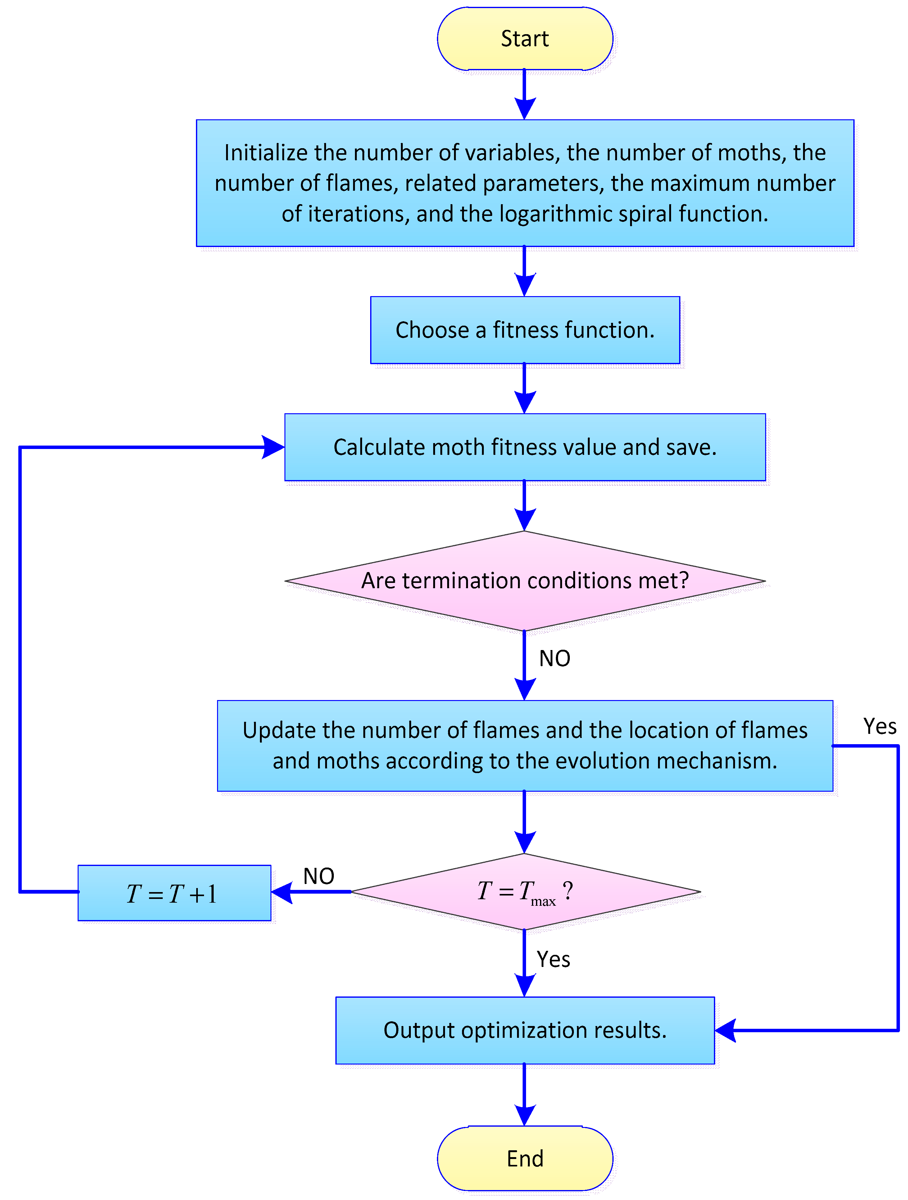
3. The Modified Moth Flame Algorithm

3.1. Brief Overview of MFO

The moth flame optimization (MFO) algorithm is a novel swarm intelligence optimization algorithm proposed by scholar Seyedali Mirjalili in 2015 [27]. It is inspired by the spiral flight of moths at night, as they follow the moon and adjust their flight direction accordingly. However, the artificial flame is very close compared to the moon. Maintaining a fixed angle with the artificial light would eventually generate a spiral flight path approaching the flame for moths. The MFO has strong parallel optimization ability and can explore a wide range of solution spaces. For non-convex problems such as DED with a large number of local optimal points, the MFO is more suitable. Figure 1 depicts the flowchart of the MFO algorithm.

3.1.1. Initialize Parameters

The MFO is essentially a swarm intelligence optimization algorithm. For the ED problem, the candidate solutions are denoted by $m$, that is, the moths are denoted by $m$. Moths fly in a one-dimensional or multi-dimensional manner in the feasible domain, and their flight paths are the range of the solution. The moths’ population $M$ is described as:

$$M=\left[\begin{array}{cccc}{m}_{1,1}& m_{1,2}& \cdots & m_{1,d}\\ m_{2,1}& m_{2,2}& \cdots & m_{2,d}\\ ⋮& ⋮& \ddots & ⋮\\ m_{n,1}& m_{n,2}& \cdots & m_{n,d}\end{array}\right]$$

(14)

where $n$ is the number of moths, and $d$ is the size of the dimension.

In the MFO, each moth has a corresponding flame, and the moth flies along its corresponding flame to update its position. The moth corresponds with the flame represented as $F$ by the dimension. The position of the flame is expressed as:

$$F=\left[\begin{array}{cccc}{F}_{1,1}& F_{1,2}& \cdots & F_{1,d}\\ F_{2,1}& F_{2,2}& \cdots & F_{2,d}\\ ⋮& ⋮& \ddots & ⋮\\ F_{n,1}& F_{n,2}& \cdots & F_{n,d}\end{array}\right]$$

(15)

The upper bound $ub$ and lower bound $lb$ in the search space can be given as follows:

$$ub=[u{b}_1,u{b}_2,u{b}_3,\cdots \cdots ,u{b}_{n-1},u{b}_n]$$

(16)

$$lb=[l{b}_1,l{b}_2,l{b}_3,\cdots \cdots ,l{b}_{n-1},l{b}_n]$$

(17)

3.1.2. The Moth’s Location Updating

The moth flies following the logarithmic spiral function $S$, which is constructed as:

$$S(M_i,F_i)=D_i{e}^{bt}\cos (2\pi t)+F_j$$

(18)

where $b$ is the parameter of the logarithmic spiral shape, and $t\in [-1,1]$ is the distance parameter. The value $t$ is proportionate to the distance of the moth relative to the flame. If $t=1$, the moth is far away from the flame, and if $t=-1$, the distance of the moth relative to the flame is very short, so the flying domain of the moth is the entire global space, including the flame itself and the space occupied by the flame. The variable $K$ can be introduced into the value of the path coefficient $t$, where $K\in [-1,-2]$. Therefore, the value range of $t$ is $t\in [K,1]$. As the number of iterations increases, the value of $K$ changes linearly from big to small, which improves the efficiency of moths approaching the flames.

$D_i$ is the distance from the ith moth to the jth flame and formulated as:

$$D_i=|F_j-M_i|$$

(19)

where $F_j$ is the $j\mathrm{t}\mathrm{h}$ flame. The number of flames $flame\_no$ needs to be adaptively updated to reduce calculation time and improve operating efficiency, which is updated by:

$$flame\_no=round(N-k\times \frac{N-1}{T})$$

(20)

where $k$ is the current iteration number, $N$ is the maximum number of flames, and $T$ is the maximum number of iterations.

The position update mechanism of the MFO is critical to unlocking its full local search capabilities. So, the optimal position generated by the moth in the previous iteration should be updated in the current iteration, meaning that if the fitness value is better than the flame, the position of the flame is updated. In each iteration, the position of the flame is saved in the matrix $F$, and then the moth updates the position according to the matrix $F$; the update mechanism $M_i$ is expressed as:

$$M_i=S(M_i,F_j)$$

(21)

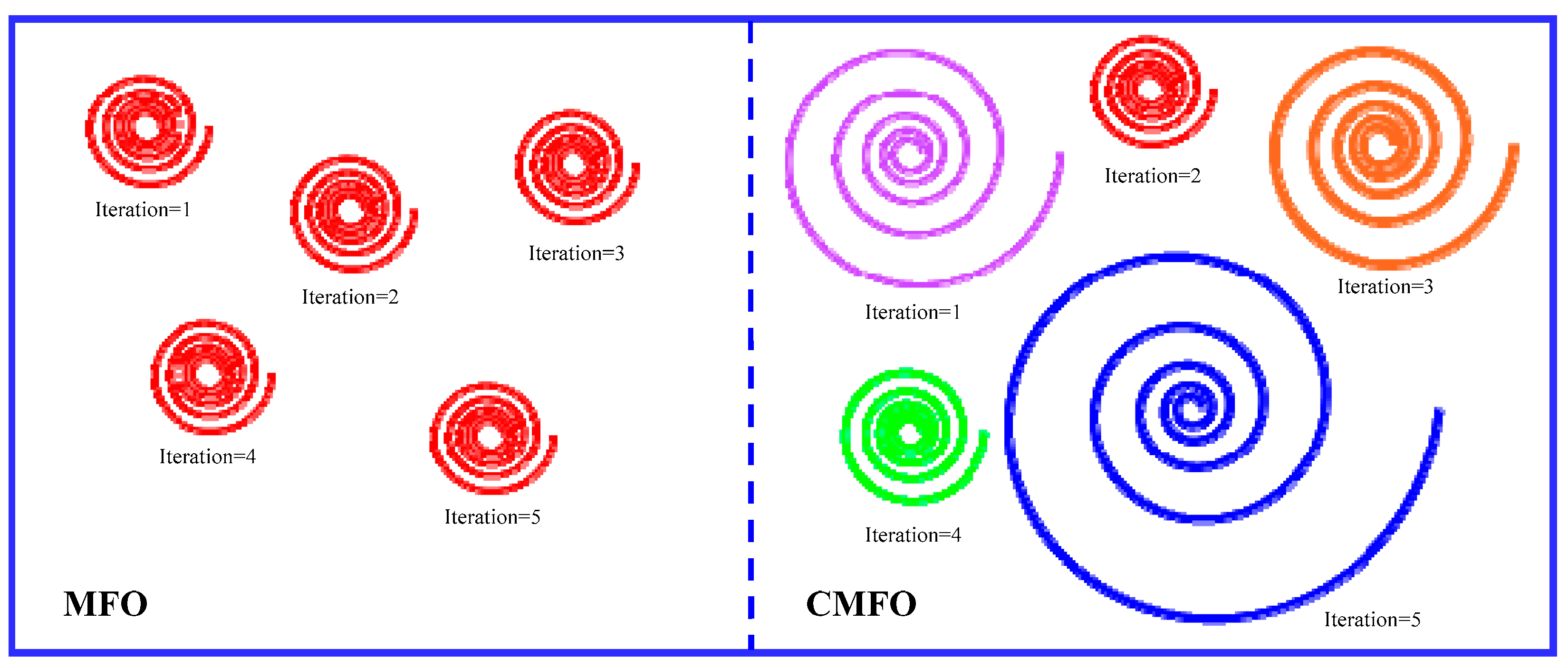
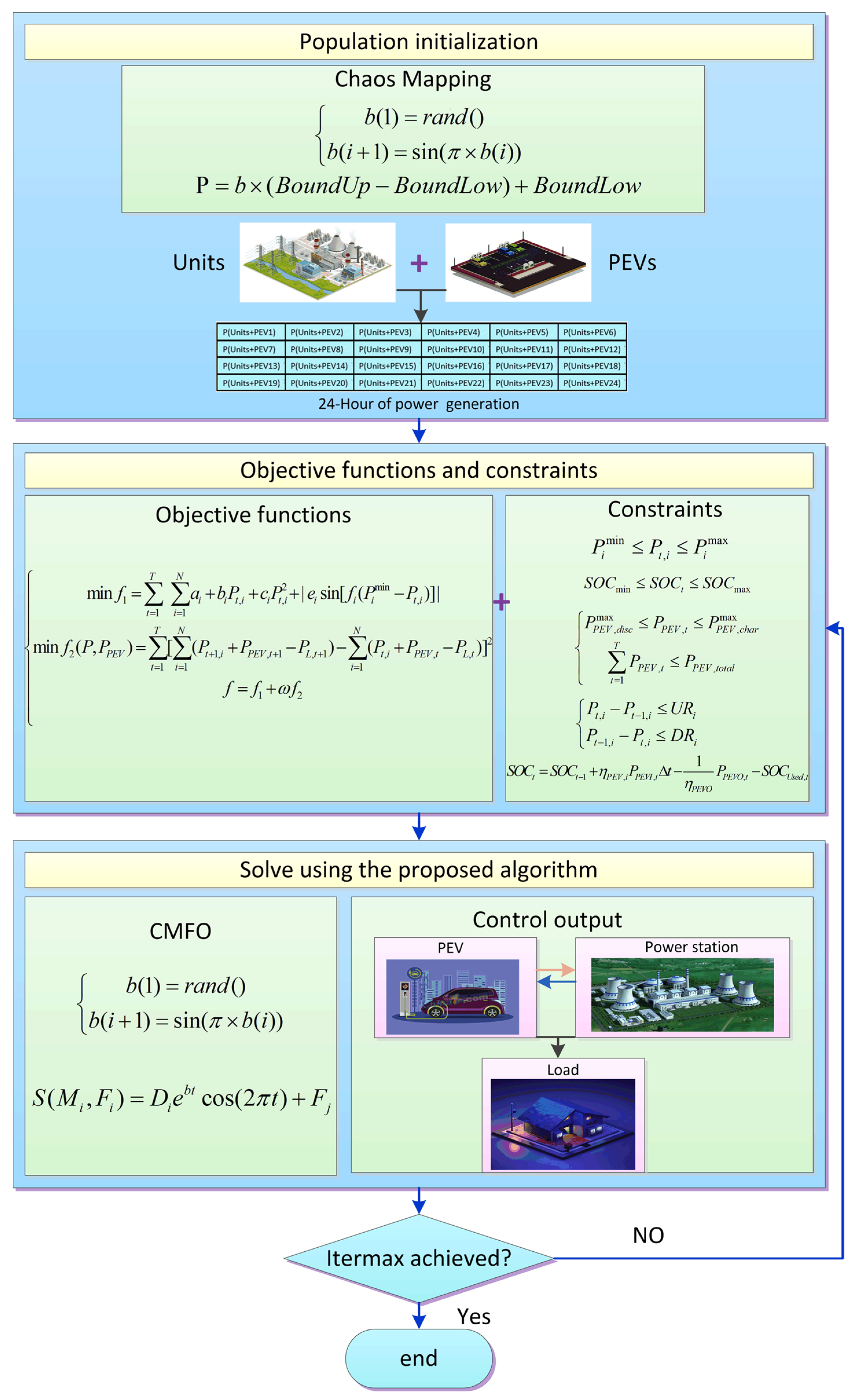
3.2. Chaos Moth Flame Algorithm

The chaos moth flame (CMFO) algorithm is an enhanced version of the MFO algorithm [27]. It integrates chaotic mapping with the evolutionary mechanism of the MFO to produce improved results. The CMFO algorithm uses a chaotic sequence, generated through chaotic mapping, to initialize the solution space and enhance the search process. As a result, the CMFO algorithm is able to obtain better initial solutions compared with the MFO algorithm. The pseudo-code for the CMFO algorithm is presented in Algorithm 1.

Algorithm 1. Chaos moth flame optimization
Input:	Population size $NP=30$.
Output:	The final solution $X_{best}$ and its fitness $f_{best}$.
1:	Set the iteration $FEs=1$ and maximum iteration $Max\_FEs$;
2:	for $i=1 to dim$
3:	for $j=1 to NP$
4:	Introduce chaotic mapping using Equation (23);
5:	Initialize the upper boundary and the lower boundary $\left(ub,lb\right)$;
6:	Initialize the position of the $i\mathrm{t}\mathrm{h}$ particle $X_{ij}$ and use mapping;
7:	end for
8:	end for
9:	While $FES<=Max\_FES do$
10:	Adaptively update the number of $flame\_no$ using Equation (20);
11:	for $i=1 to dim$
12:	Check if moths go out of the search space through $\left(ub,lb\right)$ and bring it back;
13:	Calculate the fitness of moths $f(X_{ij})$;
14:	end for
15:	if  $FES==1$
16:	Sort the first population of moths $f(X_{best})$;
17:	Update the flames $best\_flame\_ f(X_{ij})$;
18:	else
19:	Re-combinate the moth and flame; Calculate the $double\_fitness(moth\_f(X_{ij}),flame\_f(X_{ij}))$;
20:	Sort the re-combinate population $double\_fitness$;
21:	Update the flames $flame\_f(X_{best})$ using Equation (21);
22:	end if
23:	Calculate parameter a using the relevant formula;
24:	for $i=1 to dim$
25:	Calculate parameter b using chaotic mapping through Equation (23);
26:	for $j=1 to NP$
27:	if  $i<=Flame\_no$
28:	Calculate the distance between the moth and the flame $D_{ij}$ using Equation (19);
29:	Calculate the path coefficient $t$ using the relevant formula;
30:	Update the position $X_{ij}$ using Equation (18), Equation (23);
31:	end if
32:	if  $i>Flame\_no$
33:	Calculate the distance between the moth and the flame $D_{ij}$ using Equation (19);
34:	Calculate the path coefficient $t$ using the relevant formula;
35:	Update the position $X_{ij}$ using Equation (21), Equation (23);
36:	end if
37:	end for
38:	end for
39:	Update the global best position $X_{best}$ and its fitness $f_{best}$$; FES=FES+1$;
40:	end while

Chaos Mapping

Chaos is a complex and ubiquitous phenomenon in non-linear deterministic systems, where it showcases the interplay between order and disorder, determinism, and randomness [7]. Chaos is limited to a specific region, is unique and never repeats, and its orbit is complex. Although it appears random, chaos is in fact a deterministic system [14], where the state of the system at any moment is influenced by its previous state. This makes chaos unpredictable and seemingly random, yet it also exhibits good autocorrelation and low-frequency broadband, making it distinct from periodic and quasi-periodic motion. Chaos is characterized by its extreme sensitivity to initial conditions, which is one of its most prominent features. The chaotic map is described by different probability distributions that can be quantified using a probability density function. In order to measure the chaotic degree [17] of the dynamic system, $LE$ is introduced, which is used to evaluate the chaotic degree of the system as follows:

$$LE=\underset{}{{\displaystyle \underset{n\to \infty }{\lim }}}\frac{1}{n}{\displaystyle \sum _{k=1}^n\ln |f^{\prime }(x_k)|}$$

(22)

For all one-dimensional chaotic maps, $LE>0$, the three chaotic maps introduced are sine map, iterative map, chebyshev map, and correlation chaos map in

Table 1. Chaotic maps.

NO.	Chaotic Map Equations	LE
1.	Sine map: $\{\begin{array}{c}{X}_{K+1}=(a/4)\cdot \sin (\pi X_k)\\ 0<a\le 4,a=4,X_k\in (0,1)\end{array}$	0.6885
2.	Iterative map: $\{\begin{array}{c}{X}_{K+1}=\sin (a/X_k)\\ a\in (0,\infty ),a=2,X_k\in [-1,1]/\left\{0\right\}\end{array}$	1.6556
3.	Chebyshev: $\{\begin{array}{c}{X}_{K+1}=\cos (a\cdot {\cos }^{-1}{X}_k)\\ a>0,a=3,X_k\in [-1,1]\end{array}$	1.0986

.

Since the parameters of the logarithmic helix are fixed, the shape of the logarithmic helix is also fixed for MFO [27], which makes the local search ability worse. So, MFO deals with problems with high dimensionality and non-convex, which tend to get stuck in local optima. Here, the chaotic map is introduced to the evolution mechanism of the logarithmic spiral, which makes the parameters of the logarithmic spiral change in a chaotic shape in the iteration process of the CMFO. So, it makes CMFO search more comprehensively in the solution space and has strong global exploration ability. In addition, the chaotic map sequence is applied to the initialization process of CMFO, so that the CMFO has a better initial solution, which can reduce the running time of the algorithm and accelerate the convergence speed. The search principles of MFO and CMFO on the solution space are shown in Figure 2.

In Figure 2, for MFO [27], the moth needs to construct a logarithmic spiral by Equation (18) during the search process. Among the parameters of the logarithmic spiral function, the parameter $b$ determines the shape of the logarithmic spiral and is a static parameter. As can be seen from the MFO of Figure 2, the static parameter $b$ is weakly adaptive, causing the MFO to poorly explore the solution space.

The chaotic map is applied to the logarithmic spiral evolution mechanism, which is formulated by Equation (23), so that the parameter $b$ can change in a chaotic state with the iteration. The parameter $b$ is improved to a dynamic chaotic parameter. Taking the two-dimensional solution space as an example, it can be seen from the CMFO of Figure 2 that the application of the dynamic chaos parameter makes the shape of the helix change continuously with the iterations, which is highly adaptive and more exploratory to the solution space. Therefore, CMFO can well-compensate for the deficiencies of MFO.

In addition, to make the CMFO better converge to the optimal solution, the chaotic mapping sequence is used to generate the initial solution, thereby saving the running time of the CPU. Meanwhile, sine chaotic mapping is used for updating the parameter $b$. The mathematical model of the logarithmic spiral search of CMFO is described as:

$$\{\begin{array}{c}S(M_i,F_i)=D_i{e}^{b_{i}t}\cos (2\pi t)+F_j\\ b_{i+1}=\sin (\pi b_i)\end{array}$$

(23)

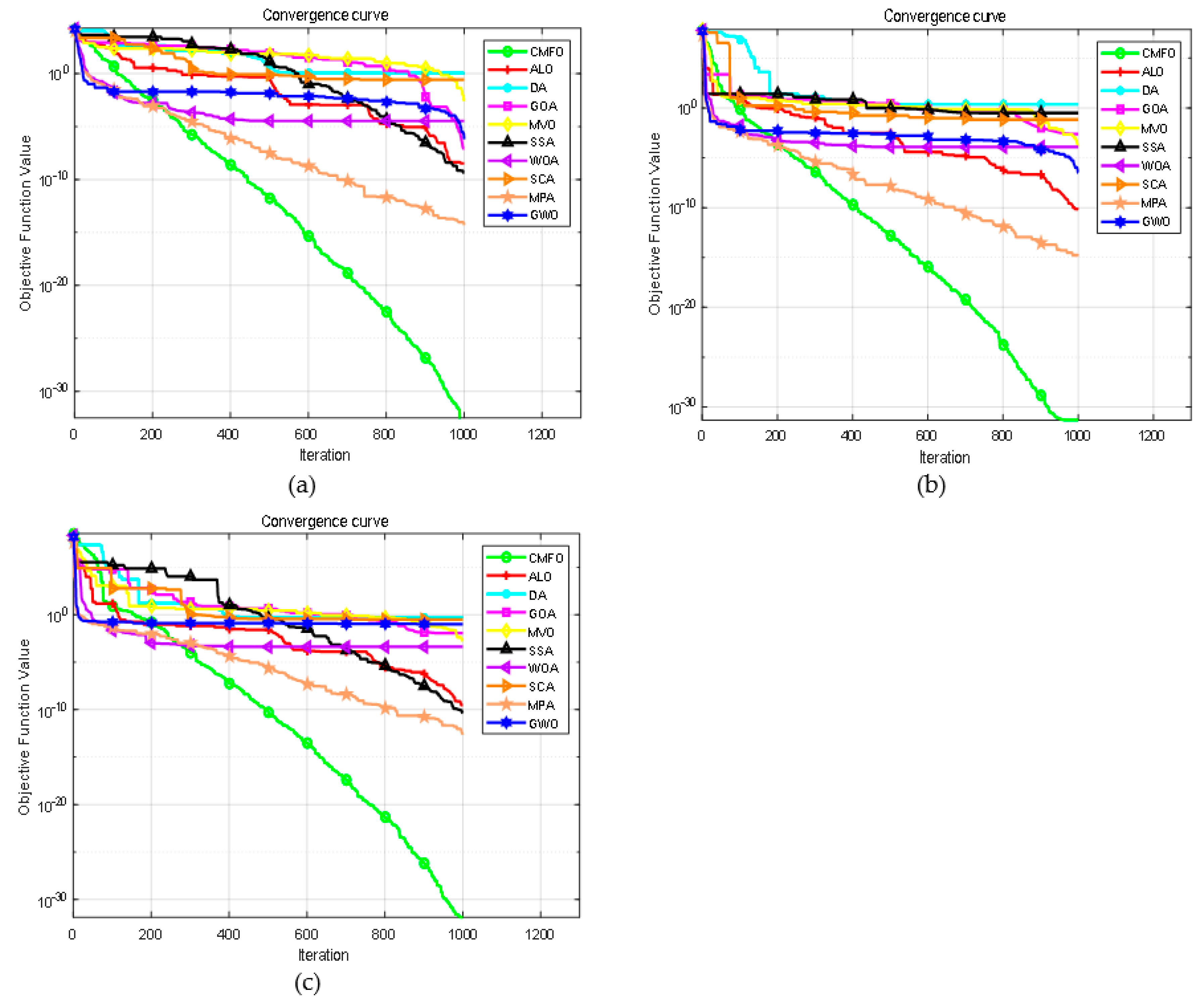
4. Performance Verification of CMFO

In order to verify the rationality and validity of the CMFO, it is compared with nine other meta-heuristic algorithms, of which the abbreviations and parameters are shown in

Table 2. List of algorithm abbreviations.

Table of Abbreviations		Abbreviation
1.	Moth-Flame Optimization Algorithm	MFO [27]
2.	Dragonfly Algorithm	DA [28]
3.	Multi-Verse Optimizer	MVO [29]
4.	Sine Cosine Algorithm	SCA [30]
5.	Ant Lion Optimizer	ALO [31]
6.	Grasshopper Optimisation Algorithm	GOA [32]
7.	Salp Swarm Algorithm	SSA [33]
8.	Whale Optimization Algorithm	WOA [34]
9.	Ocean Predator Algorithm	MPA [35]
10.	Grey Wolf Optimizer	GWO [36]
11.	Chaos Moth-Flame Optimization Algorithm	CMFO

and

Table 3. The parameters of the algorithms.

Algorithms	Parameter Settings	Iteration
MFO [27]	NP = 30	1000, 10,000
DA [28]	NP = 30, Beta = 1.5	1000, 10,000
MVO [29]	NP = 30, WEP_Max = 1, WEP_min = 0.2	1000, 10,000
SCA [30]	NP = 30, a = 2	1000, 10,000
ALO [31]	NP = 30	1000, 10,000
GOA [32]	NP = 30, Cmax = 1, Cmin = 0.00004	1000, 10,000
SSA [33]	NP = 30	1000, 10,000
WOA [34]	NP = 30, b = 1	1000, 10,000
MPA [35]	NP = 30, Fads = 0.2, P = 0.5, Beta = 1.5	1000, 10,000
GWO [36]	NP = 30	1000, 10,000
CMFO	NP = 30	1000, 10,000

, respectively. The above experiments are performed by conducting on seven well-known benchmark functions, which are F1 (Sphere), F2 (Schwelfel’s 2.22), F3 (Schwelfel’s 1.2), F4 (Step), F5 (Griewank), F6 (Ackley), F7 (Penalized-1), as shown in

Table 4. Benchmark functions.

Function	Dim	Range	${\mathit{F}}_{\mathbf{min}}$
$F_1(x)={\displaystyle \sum _{i=1}^n{x}_i^2}$	$10/20/50$	$[-100,100]$	$0$
$F_2(x)={\displaystyle \sum _{i=1}^n\left|x_i\right|}+{\displaystyle \prod _{i=1}^n\left|x_i\right|}$	$10/20/50$	$[-100,100]$	$0$
$F_3(x)={\displaystyle \sum _{i=1}^n({\displaystyle \sum _{j=1}^i{x}_j}{)}^2}$	$10/20/50$	$[-100,100]$	$0$
$F_4(x)={\displaystyle \sum _{i=1}^n{([x_i+0.5])}^2}$	$10/20/50$	$[-100,100]$	$0$
$F_5(x)=\frac{1}{4000}{\displaystyle \sum _{i=1}^n{x}_i{}^2}-{\displaystyle \prod _{i=1}^n\cos (\frac{x_i}{\sqrt{i}})+1}$	$10/20/50$	$[-600,600]$	$0$
$\{\begin{array}{c}{F}_6(x)=\frac{\pi }{n}\{10\sin (\pi y_1)+{\displaystyle \sum _{i=1}^{n-1}{(y_i-1)}^2}[1+10{\sin }^2(\pi y_{i+1})]+{(y_n-1)}^2\}+{\displaystyle \sum _{i=1}^{n}u(x_i,10,100,4)}\\ y_i=1+\frac{x_i+1}{4}\end{array}$	$10/20/50$	$[-50,50]$	$0$
$F_7(x)=0.1\{{\sin }^2(3\pi x_i)+{\displaystyle \sum _{i=1}^n{(x_i-1)}^2[1+{\sin }^2(3\pi x_i+1)]+{(x_n-1)}^2[1+{\sin }^2(2\pi x_n)]}\}+{\displaystyle \sum _{i=1}^{n}u(x_i,5,100,4)}$	$10/20/50$	$[-50,50]$	$0$

, which include unimodal and multimodal functions. Because of only one optimum, the solution of unimodal function can be determined easily. However, for the multimodal function, the number of local minimum increases with the dimension of problems, thus it is difficult to obtain optimal solutions. Therefore, the selected benchmark functions can effectively evaluate the performance of the algorithm in terms of escaping from the local optimum and convergence speed. Furthermore, three dimensions, namely 10, 20, and 50, are selected to test the generalization ability of the algorithm, and each trial runs 30 times independently. For the test case of 10 dimensions and 20 dimensions, the number of iterations is 1000. For the test case of 50 dimensions, the number of iterations is 10,000. All experiments in this study are conducted in a PC with MATLAB ^®2020a, Intel(R) Core (TM) i5-7200U CPU @ 2.50 GHz(4CPUs), and RAM 8.0 GHz. The experiment results are shown in

Table 5. Comparison of CMFO with other algorithms (10 dimensions).

NO.	Statistics	ALO	DA	GOA	MVO	SSA	WOA	SCA	MPA	GWO	MFO	CMFO
F1	Sta	1.40 × 10−9	2.34 × 101	1.50 × 10−7	1.80 × 10−3	3.30 × 10−10	4.24 × 10−155	4.74 × 10−25	2.93 × 10−63	9.89 × 10−133	9.46 × 10−22	2.06 × 10−34
	Best	8.42 × 10−10	2.50 × 10−3	6.37 × 10−8	1.20 × 10−3	4.13 × 10−10	1.70 × 10−175	3.69 × 10−34	2.89 × 10−65	4.91 × 10−123	1.30 × 10−20	1.55 × 10−36
	Time(s)	1.45 × 101	3.64 × 101	5.77 × 101	8.44 × 10−1	3.65 × 10−1	9.44 × 10−1	4.45 × 10−1	8.86 × 10−1	6.34 × 10−1	3.91 × 10−1	3.58 × 10−1
	Winner	N	N	N	N	N	Y	N	Y	Y	N	+
F2	Sta	1.34 × 100	1.12 × 100	8.08 × 101	1.16 × 10−2	9.19 × 10−6	9.27 × 10−106	1.20 × 10−18	5.90 × 10−35	7.86 × 10−67	1.01 × 10−13	1.50 × 10−20
	Best	1.44 × 10−5	6.91 × 10−1	2.01 × 102	8.10 × 10−3	4.58 × 10−6	3.15 × 10−116	7.80 × 10−22	1.13 × 10−36	7.54 × 10−69	2.56 × 10−15	2.84 × 10−22
	Time(s)	1.42 × 101	3.85 × 101	5.99 × 101	9.15 × 10−1	4.09 × 10−1	1.26 × 100	4.56 × 10−1	9.50 × 10−1	6.68 × 10−1	4.51 × 10−1	4.38 × 10−1
	Winner	N	N	N	N	N	Y	N	Y	Y	N	+
F3	Sta	8.10 × 10−6	6.02 × 101	1.02 × 10−1	1.42 × 10−2	1.24 × 10−9	2.86 × 101	5.45 × 10−8	3.07 × 10−31	1.08 × 10−53	1.27 × 10−5	1.10 × 10−10
	Best	2.22 × 10−6	2.19 × 100	1.62 × 10−4	4.80 × 10−3	6.00 × 10−10	9.64 × 10−6	3.68 × 10−13	3.56 × 10−36	2.59 × 10−61	3.97 × 10−3	3.60 × 10−13
	Time(s)	1.42 × 101	3.89 × 101	6.48 × 101	1.05 × 100	5.66 × 10−1	1.31 × 100	5.43 × 10−1	1.33 × 100	8.57 × 10−1	6.01 × 10−1	5.83 × 10−1
	Winner	N	N	N	N	N	N	N	Y	Y	N	+
F4	Sta	6.63 × 10−10	1.33 × 101	2.66 × 10−7	1.70 × 10−3	3.16 × 10−10	8.42 × 10−5	9.86 × 10−2	9.99 × 10−15	1.97 × 10−7	2.19 × 10−10	0.00 × 100
	Best	9.24 × 10−10	1.58 × 10−2	3.59 × 10−8	1.20 × 10−3	2.11 × 10−10	1.04 × 10−5	1.70 × 10−1	4.39 × 10−16	4.86 × 10−7	3.92 × 10−17	0.00 × 100
	Time(s)	1.28 × 100	3.62 × 101	5.92 × 101	9.10 × 10−1	4.06 × 10−1	8.38 × 10−1	4.35 × 10−1	9.45 × 10−1	6.17 × 10−1	3.97 × 10−1	3.92 × 10−1
	Winner	N	N	N	N	N	N	N	N	N	N	+
F5	Sta	9.07 × 10−2	3.01 × 10−1	1.19 × 10−1	9.36 × 10−2	9.78 × 10−2	1.42 × 10−1	9.45 × 10−2	9.87 × 10−2	1.19 × 10−1	4.9748	9.04 × 10−2
	Best	3.20 × 10−2	1.51 × 10−1	1.40 × 10−1	8.48 × 10−2	4.93 × 10−2	0.00 × 100	0.00 × 100	0.00 × 100	0.00 × 100	16.1056	0.00 × 100
	Time(s)	1.42 × 101	3.67 × 101	6.47 × 101	1.00 × 100	4.84 × 10−1	1.04 × 100	4.95 × 10−1	1.27 × 100	6.90 × 10−1	4.72 × 10−1	4.91 × 10−1
	Winner	N	N	N	N	N	N	N	N	N	N	+
F6	Sta	6.95 × 10−1	1.35 × 100	8.90 × 10−1	1.43 × 10−1	2.67 × 10−1	4.00 × 10−3	2.54 × 10−2	2.77 × 10−15	7.86 × 10−3	0.2801	9.47 × 10−33
	Best	2.58 × 10−11	5.80 × 10−2	6.07 × 10−6	1.56 × 10−5	5.12 × 10−12	2.28 × 10−5	3.32 × 10−2	4.25 × 10−16	1.20 × 10−7	2.37 × 10−7	4.71 × 10−32
	Time(s)	1.46 × 101	3.68 × 101	6.12 × 101	1.35 × 100	8.62 × 10−1	1.82 × 100	8.78 × 10−1	1.87 × 100	1.05 × 100	9.49 × 10−1	8.88 × 10−1
	Winner	N	N	N	N	N	N	N	N	N	N	+
F7	Sta	4.39 × 10−3	2.18 × 10−1	1.35 × 10−2	5.40 × 10−3	4.40 × 10−3	2.61 × 10−2	6.93 × 10−2	1.18 × 10−13	3.98 × 10−2	1.47 × 10−5	6.92 × 10−32
	Best	1.04 × 10−10	3.56 × 10−2	4.19 × 10−6	1.11 × 10−4	2.12 × 10−11	7.70 × 10−5	1.86 × 10−1	7.23 × 10−15	1.00 × 10−6	3.79 × 10−8	1.35 × 10−32
	Time(s)	1.69 × 101	3.67 × 101	6.55 × 101	1.36 × 100	9.12 × 10−1	1.85 × 100	9.01 × 10−1	1.85 × 100	1.15 × 100	8.71 × 10−1	8.35 × 10−1
	Winner	N	N	N	N	N	N	N	N	N	N	+

,

Table 6. Scenarios.

Scenario 1: Only Units	Dimensions	Scenario 2: Units with PEVs	Dimensions
Case Ⅰ: 5 units	5 × 24 = 120	Case Ⅳ: 5 units + PEVs	6 × 24 = 144
Case Ⅱ: 10 units	10 × 24 = 240	Case Ⅴ: 10 units + PEVs	11 × 24 = 264
Case Ⅲ: 15 units	15 × 24 = 360	Case Ⅵ: 15 units + PEVs	16 × 24 = 384

and

Table 7. Comparison of whether PEVs in DED.

Parameter	Best Cost ($)	Worst Cost ($)	Average Cost ($)	Fluctuation (MW)^2	Sta	CPU Time (s)
Scenario 1
caseⅠ: 5 units	3.98 × 104	4.07 × 104	3.99 × 104	1.06 × 106	6.67 × 102	2.65 × 102
caseⅡ: 10 units	2.28 × 106	2.31 × 106	2.29 × 106	1.97 × 106	4.85 × 104	9.57 × 102
caseⅢ: 15 units	6.71 × 105	6.95 × 105	6.74 × 105	2.09 × 106	9.67 × 103	2.05 × 103
Scenario 2
caseⅣ: 5 units	3.93 × 104	4.19 × 104	4.07 × 104	7.90 × 105	8.87 × 102	2.33 × 102
caseⅤ: 10 units	2.17 × 106	2.33 × 106	2.25 × 106	1.01 × 106	3.90 × 104	9.30 × 102
caseⅥ: 15 units	6.50 × 105	6.83 × 105	6.71 × 105	1.16 × 106	9.00 × 103	1.97 × 103

, which are in terms of the standard deviation “Sta”, optimal value “Best” of the best-so-far solution, and average CPU running time “Time(s)”.

In Table 5,

Table A1. Comparison of CMFO with other algorithms (20 dimensions).

NO.	Statistics	ALO	DA	GOA	MVO	SSA	WOA	SCA	MPA	GWO	MFO	CMFO
F1	Sta	2.12 × 10−8	3.83 × 102	3.51 × 10−2	1.67 × 10−2	5.81 × 10−10	6.02 × 10−154	4.47 × 10−8	1.7 × 10−52	5.18 × 10−75	6.85 × 10−8	1.12 × 10−11
	Best	2.17 × 10−8	1.22 × 102	6.54 × 10−4	4.64 × 10−2	2.87 × 10−9	7.49 × 10−167	5.93 × 10−11	1.0 × 10−57	2.39 × 10−78	3.05 × 10−6	1.80 × 10−13
	Time(s)	3.65 × 101	6.78 × 101	1.16 × 102	1.29 × 100	4.39 × 10−1	1.13 × 100	6.39 × 10−1	1.03 × 100	9.41 × 10−1	1.39 × 100	1.15 × 100
	Winner	N	N	N	N	N	Y	N	Y	Y	N	+
F2	Sta	1.93 × 101	3.09 × 100	2.95 × 1015	1.52 × 10−2	4.76 × 10−1	9.18 × 10−102	3.51 × 10−9	5.9 × 10−29	1.13 × 10−43	1.72 × 10−6	4.07 × 10−9
	Best	1.13 × 10−2	3.41 × 100	2.51 × 102	7.71 × 10−2	5.53 × 10−5	1.71 × 10−113	2.11 × 10−11	1.4 × 10−32	4.94 × 10−45	8.00 × 10−5	8.16 × 10−10
	Time(s)	4.10 × 101	8.22 × 101	1.29 × 102	1.38 × 100	5.00 × 10−1	1.22 × 100	6.54 × 10−1	1.23 × 100	1.05 × 100	10.31 × 10−1	9.85 × 10−1
	Winner	N	N	N	N	N	Y	Y	Y	Y	N	+
F3	Sta	5.36 × 101	2.53 × 103	8.77 × 101	1.32 × 100	7.71 × 10−1	1.93 × 103	2.81 × 102	5.0 × 10−18	2.66 × 10−23	11.8826	6.59 × 100
	Best	8.58 × 100	4.35 × 102	3.15 × 101	6.35 × 10−1	2.62 × 10−2	2.72 × 102	1.92 × 10−1	4.5 × 10−27	2.51 × 10−30	3.99 × 103	7.84 × 10−1
	Time(s)	4.27 × 101	9.03 × 101	1.29 × 102	1.65 × 100	8.20 × 10−1	1.76 × 100	9.26 × 10−1	1.95 × 100	1.36 × 100	1.57 × 100	1.52 × 100
	Winner	N	N	N	N	N	N	N	Y	Y	N	+
F4	Sta	2.83 × 10−8	1.41 × 100	3.51 × 10−2	2.19 × 10−2	1.35 × 10−9	1.56 × 10−2	1.71 × 10−1	7.40 × 10−11	1.23 × 10−1	4.02 × 10−4	3.24 × 10−11
	Best	2.35 × 10−8	3.18 × 10−1	8.17 × 10−4	2.75 × 10−2	1.82 × 10−9	7.99 × 10−4	1.68 × 100	4.58 × 10−11	2.21 × 10−6	5.13 × 10−8	8.78 × 10−13
	Time(s)	4.19 × 101	6.20 × 101	1.55 × 102	1.47 × 100	5.09 × 10−1	1.17 × 100	6.22 × 10−1	1.17 × 100	1.03 × 100	9.99 × 10−1	9.72 × 10−1
	Winner	N	N	N	N	N	N	N	N	N	N	+
F5	Sta	2.85 × 10−2	9.47 × 10−1	9.49 × 10−2	7.82 × 10−2	1.31 × 10−2	0.00 × 100	2.32 × 10−1	0.00 × 100	0.00 × 100	52.8037	1.60 × 10−12
	Best	5.38 × 10−6	8.84 × 10−1	3.78 × 10−2	1.29 × 10−1	1.34 × 10−8	0.00 × 100	1.63 × 10−9	0.00 × 100	0.00 × 100	40.6902	4.66 × 10−13
	Time(s)	4.23 × 101	6.89 × 101	1.91 × 102	1.54 × 100	5.85 × 10−1	1.31 × 100	7.00 × 10−1	1.28 × 100	1.11 × 100	1.20 × 100	1.09 × 100
	Winner	N	N	N	N	N	Y	N	Y	Y	N	+
F6	Sta	2.62 × 100	5.89 × 100	1.96 × 100	4.90 × 10−1	9.69 × 10−1	2.54 × 10−3	1.17 × 10−1	1.31 × 10−11	1.53 × 10−2	3.0935	3.10 × 10−10
	Best	4.37 × 10−1	7.08 × 10−1	1.04 × 100	6.52 × 10−4	3.30 × 10−1	3.81 × 10−4	2.50 × 10−1	5.06 × 10−12	9.72 × 10−3	6.47 × 10−5	1.77 × 10−12
	Time(s)	4.29 × 101	7.69 × 101	2.01 × 102	1.93 × 100	1.07 × 100	2.21 × 100	1.16 × 100	2.30 × 100	1.58 × 100	1.79 × 100	1.82 × 100
	Winner	N	N	N	N	N	N	N	N	N	N	+
F7	Sta	7.16 × 10−3	8.54 × 100	8.36 × 10−2	1.65 × 10−2	4.39 × 10−3	8.02 × 10−2	6.16 × 10−2	8.67 × 10−11	1.26 × 10−1	7.86 × 10−4	5.12 × 10−11
	Best	3.96 × 10−8	1.49 × 100	4.09 × 10−3	5.97 × 10−3	1.75 × 10−10	7.50 × 10−3	1.17 × 100	4.80 × 10−11	1.37 × 10−5	3.29 × 10−7	1.34 × 10−11
	Time(s)	4.27 × 101	7.68 × 101	2.65 × 102	1.97 × 100	1.07 × 100	2.23 × 100	1.18 × 100	2.32 × 100	1.70 × 100	1.86 × 100	1.80 × 100
	Winner	N	N	N	N	N	N	N	N	N	N	+

and

Table A2. Comparison of CMFO with other algorithms (50 dimensions).

NO.	Statistics	ALO	DA	GOA	MVO	SSA	WOA	SCA	MPA	GWO	MFO	CMFO
F1	Sta	2.96 × 10−27	1.92 × 102	7.30 × 10−3	7.90 × 10−3	1.93 × 10−9	0.00 × 100	1.35 × 10−16	0.00 × 100	0.00 × 100	5.35 × 10−4	5.71 × 10−38
	Best	8.27 × 10−26	5.07 × 101	1.66 × 10−2	1.47 × 10−2	9.04 × 10−9	0.00 × 100	1.01 × 10−28	0.00 × 100	0.00 × 100	0.0633	2.95 × 10−39
	Time(s)	3.71 × 103	7.07 × 102	3.13 × 103	3.18 × 101	7.46 × 100	1.73 × 101	1.20 × 101	2.46 × 101	22.47876667	9.991	9.828
	Winner	N	N	N	N	N	Y	N	Y	Y	N	+
F2	Sta	3.5048 × 10−6	2.99 × 100	5.41 × 1023	5.69 × 10−2	1.42 × 100	0.00 × 100	7.51 × 10−29	0.00 × 100	0.00 × 100	10	2.87 × 101
	Best	1.40 × 10−7	1.75 × 100	5.16 × 1022	1.09 × 10−1	4.20 × 10−3	0.00 × 100	4.22 × 10−42	5.92 × 10−286	3.21 × 10−277	42.4382	3.31 × 10−22
	Time(s)	3.61 × 103	7.47 × 102	4.46 × 103	2.91 × 101	7.50 × 100	1.71 × 101	1.14 × 101	2.37 × 101	2.25 × 101	1.11 × 101	1.07 × 101
	Winner	N	N	N	N	N	Y	Y	Y	Y	N	+
F3	Sta	7.83 × 10−1	8.91 × 103	6.58 × 101	6.90 × 10−3	1.43 × 10−4	3.53 × 103	7.62 × 103	6.20 × 10−118	3.02 × 10−103	2.50 × 104	1.95 × 104
	Best	4.02 × 100	7.91 × 103	7.46 × 102	9.97 × 100	1.58 × 10−5	2.75 × 100	5.69 × 102	9.46 × 10−170	7.69 × 10−125	1.69 × 104	3.83 × 10−1
	Time(s)	4.07 × 104	9.24 × 102	3.25 × 103	3.67 × 101	1.62 × 101	3.19 × 101	1.91 × 101	5.05 × 101	3.18 × 101	1.81 × 101	1.73 × 101
	Winner	N	N	N	N	Y	N	N	Y	Y	N	+
F4	Sta	5.88 × 10−9	1.71 × 102	1.58 × 10−1	2.11 × 10−2	2.11 × 10−9	2.77 × 10−5	3.65 × 10−1	1.50 × 10−12	7.87 × 10−1	8.94 × 10−2	2.62 × 10−28
	Best	8.62 × 10−8	5.19 × 102	2.37658 × 10−6	1.61 × 10−2	8.49 × 10−9	4.51 × 10−5	7.63 × 100	3.38 × 10−12	7.42 × 10−1	9.15 × 10−7	3.89 × 10−30
	Time(s)	3.95 × 103	6.28 × 102	3.28 × 103	3.07 × 101	7.52 × 100	2.13 × 101	1.12 × 101	2.36 × 101	2.24 × 101	10.06 × 100	9.54 × 100
	Winner	N	N	N	N	N	N	N	N	N	N	N
F5	Sta	5.80 × 10−5	1.05 × 100	9.34 × 10−8	6.50 × 10−2	7.20 × 10−3	3.00 × 10−3	1.17 × 10−1	0.00 × 100	0.00 × 100	219.95	0.00 × 100
	Best	1.51 × 10−8	1.79 × 100	1.0899 × 10−8	5.51 × 10−2	1.76 × 10−8	0.00 × 100	0.00 × 100	0.00 × 100	0.00 × 100	40.93	0.00 × 100
	Time(s)	3.99 × 103	6.96 × 102	3.29 × 103	3.21 × 101	8.67 × 100	2.03 × 101	1.21 × 101	2.60 × 101	2.31 × 101	1.20 × 101	1.15 × 101
	Winner	N	N	N	N	N	N	N	N	N	N	+
F6	Sta	2.66 × 100	1.84 × 100	1.6563 × 10−7	1.04 × 100	2.13 × 100	2.15 × 10−6	4.02 × 10−1	5.11 × 10−14	2.09 × 10−2	9.55	2.69 × 10−28
	Best	8.02 × 100	4.59 × 100	1.10373 × 10−8	1.01 × 10−4	8.16 × 10−2	2.84 × 10−6	4.98 × 10−1	1.00 × 10−14	4.33 × 10−2	8.03 × 10−9	5.01 × 10−32
	Time(s)	4.09 × 104	8.24 × 102	3.32 × 103	3.79 × 101	1.72 × 101	3.49 × 101	2.05 × 101	4.67 × 101	3.20 × 101	1.95 × 101	1.90 × 101
	Winner	N	N	N	N	N	N	N	N	N	N	+
F7	Sta	5.20 × 10−3	9.55 × 100	1.52238 × 10−7	5.30 × 10−3	5.40 × 10−3	4.10 × 10−3	5.33 × 100	3.30 × 10−3	3.19 × 10−1	3.75 × 10−2	3.81 × 10−27
	Best	5.96 × 10−9	1.65 × 101	5.83674 × 10−9	1.70 × 10−3	4.06 × 10−10	6.05 × 10−5	3.79 × 100	2.93 × 10−12	1.00 × 100	1.94 × 10−7	1.38 × 10−30
	Time(s)	3.91 × 104	1.25 × 103	4.63 × 103	4.00 × 101	1.80 × 101	3.42 × 101	2.06 × 101	4.66 × 101	3.21 × 101	2.04 × 101	1.98 × 101
	Winner	N	N	N	N	N	N	N	N	N	N	+

, in Appendix A, among the three metrics “Sta”, “Best”, and “Time”, N means that the algorithm is worse than the CMFO in more than two metrics, and Y means that the algorithm is better than the CMFO in more than two metrics. Furthermore, ‘+’ means that the performance of the algorithm is superior. Table 5, Table A1 and Table A2, in Appendix A, show that the proposed CMFO is better than the other algorithms except for WOA [34], MPA [35], and GWO [36], according to the statistical results. In particular, the small optimal value and standard deviation of different kinds of functions indicate that the CMFO has high solution precision and stability. Furthermore, compared with other methods, the CMFO significantly reduces the time of computing. For example, in 10 dimensions, the CMFO converged 305%, 916%, 1511%, 135%, 2%, 163%, 24%, 147%, 77%, and 9% faster compared with the other 10 algorithms in the unimodal test function F1, and also improved the stability of the optimal values. In the multimodal test function F6, the CMFO improves the convergence speed compared with the other 10 algorithms by 1544%, 314%, 589%, 52%, −3%, 104%, −1%, 110%, 18%, and 7%, respectively, and improves the stability and accuracy of the optimal values. In the multimodal test function F7, the CMFO converges 102%, 339%, 684%, 62%, 9%, 121%, 8%, 121%, 38%, and 4% faster than the other 10 algorithms, respectively, and also improves the accuracy of the optimal values. Moreover, the advantages of CMFO in optimizing unimodal and multimodal test functions remain when improved to 20 and 50 dimensions, indicating that the improved algorithm is equally suitable for solving high-dimensional, high-complexity optimization problems, making it a good choice to use CMFO for problems with higher dimensionality and complexity like DED.

In order to provide an intuitive comparison, the convergence curves of Step, Ackley, and Penalized-1 representatives are illustrated in Figure 3 and Figure A1 in Appendix A. It can be seen from the convergence curves that the CMFO has stronger exploration ability, faster convergence, more generality, and higher accuracy compared with other algorithms. Such improvements are related to chaotic mapping and are introduced into CMFO. Meanwhile, the experiment results fully demonstrate that the proposed CMFO is promising and competitive.

5. Implementation of CMFO to DED Problems

The conceptual representation of the CMFO approach to solving the dynamic economic dispatch problem with the integration of plug-in electric vehicles is depicted in Figure 4. This representation consists of three integral components: the initial population formation through chaotic mapping, which enhances the diversity of the population; the objective function and constraints of the DED problem, which are transformed from a multi-objective problem to a single-objective problem through weight factors; and the application of the CMFO algorithm to solve the DED problem [45].

Furthermore, the model of plug-in electric vehicles to the grid used in this paper is shown in Figure 5. The system operator determines the day-ahead schedule of thermal power plants according to the power demand as well as coordinates the power delivering/receiving to/from the PEV aggregators [46]. In plug-in electric vehicles to the grid mode, PEV aggregators are designed to possess options for delivering or receiving power to/from the grid. The model is simple and efficient, so it is used to study the DED problem.

5.1. Parameter Setting

The population size of the CMFO is NP = 500, the number of PEVs is 75,000, the charging and discharging efficiencies are both 0.85, the available PEVs are 20%, and the average battery capacity is 0.015 MW. The V2G error is 0.01, and the objective function weight value is set to 1. In addition, the charging and discharging power of PEVs is 100 MW, and for 5 units, the maximum power generation of a single unit is 300 MW; the minimum value of power generation demand for each time period is 410 MW and the maximum value is 720 MW. For 10 units, the maximum generation power of each single unit is 470 MW, and the minimum value of generation demand for each time period is 1036 MW and the maximum value is 1972 MW. For 15 units, the maximum generation power of each single unit is 470 MW, and the minimum value of generation demand for each time period is 1171 MW and the maximum value is 2394 MW. Therefore, from the power generation perspective, the power ratios of a single genset and a PEV are 3:1, 4.7:1, and 4.7:1, respectively, and the impact of a PEV is 13.9~24.4% for 5 units, 5.1~9.7% for 10 units, and 4.2~8.5% for 15 units. Therefore, the reasonable deployment of electric vehicle charging and discharging can reduce the grid fluctuation to a certain extent and achieve the effect of peak and valley reduction.

Regarding the algorithms used for comparison, for MFO [27], NP = 500 and the crossover probability PC = 0.7. For GADMFI [26], the mutation probability Pm = 0.3 and the population size NP = 100. For MPA [35], NP = 500, Fads = 0.2, P = 0.5, and Beta = 1.5. The number of iterations for each algorithm remains fixed. In order to verify the reliability of the proposed algorithm for DED problems, two scenarios and six cases are considered, as described in Table 6.

5.2. Scenarios 1 and 2

The three cases of Scenario 1 are power systems with 5 units, 10 units, and 15 units, respectively, which are used to test the performance of the CMFO. For Scenario 2, PEVs are connected to the grid to reduce the fluctuation of the power grid, and the charging mode is random charging, which is more in line with the actual situation, regardless of forcing the user to choose to discharge at peak power consumption and charge at low power consumption [47,48]. Three cases, 5 units + PEVs, 10 units + PEVs, and 15 units + PEVs, are used to test the performance of the CMFO. The experiment results of Scenarios 1 and 2 are shown in Table 7. For intuitive analysis of Units + PEVs, the output power in each period is shown in Figure 6, and the power curve in each period is shown in Figure 7. In Figure 6, the “FEVs” curve represents the charge and discharge of PEVs in each period, and the “Original Demand + FEVs” curve represents the actual power generation of the genset in each period when PEVs are engaged. The curve “Original Demand + FEVs” reduces the grid fluctuation compared with the curve “Original Demand” and achieves the effect of peak and valley reduction. Each stacked histogram in Figure 7 represents the sum of the power generation of each test case at each period, and the bars with different colors represent the power output of different units. Meanwhile, for Scenario 2, the output powers of each unit and PEVs in each period are also shown in

Table 8. Case IV: 5 units + PEVs.

Hour	U1(MW)	U2(MW)	U3(MW)	U4(MW)	U5(MW)	PEVs(MW)
1	10.0000	53.6858	175.0000	40.0000	50.0000	63.9108
2	15.7117	27.1060	31.5891	84.2206	93.7074	52.5612
3	12.3513	62.5644	32.9835	151.6454	295.3407	35.8271
4	66.4852	74.7164	45.3262	191.0710	125.7262	17.3350
5	10.3371	47.6915	149.1630	40.0000	90.4991	13.1349
6	70.0996	83.7379	102.7415	40.0000	50.0000	0.6600
7	57.0166	42.8705	30.0000	76.7857	112.7795	6.9656
8	10.0000	52.0368	30.0000	132.5563	50.0000	3.7592
9	45.5688	98.9987	30.0000	58.6576	286.4174	−3.9636
10	51.6049	43.4705	175.0000	143.2037	50.0000	−4.3255
11	10.0000	20.0000	30.0000	40.0000	155.1979	−9.3044
12	42.5523	97.3219	141.7528	172.2989	63.4971	−20.6566
13	10.0000	44.5992	30.0000	250.0000	150.2540	−3.7945
14	10.0000	118.0385	157.8564	244.6124	50.0000	2.2380
15	19.3010	33.3553	133.4780	99.8295	50.0000	15.9469
16	27.0477	20.0000	100.0908	111.1224	202.6196	49.0711
17	75.0000	124.5431	93.7788	40.0000	137.5331	55.8396
18	59.3929	68.8096	169.7482	102.9944	50.0000	26.3521
19	75.0000	53.0772	83.2589	40.0000	271.9666	−1.6668
20	10.0000	85.7967	108.6016	40.0000	101.0388	−31.0459
21	29.7327	39.2235	46.4968	40.0000	174.5293	−20.2485
22	47.7149	106.2207	153.9936	100.3830	300.0000	18.7699
23	27.1922	84.3751	30.0000	59.3461	131.1061	56.5571
24	75.0000	104.5927	39.5150	152.5159	50.0000	87.0775
Total fuel cost ($): 3.93 × 104

,

Table A3. Case Ⅴ: 10 units + PEVs.

Hour	U1(MW)	U2(MW)	U3(MW)	U4(MW)	U5(MW)	U6(MW)	U7(MW)	U8(MW)	U9(MW)	U10(MW)	PEVs(MW)
1	160.8696	135.0000	75.8791	70.4196	75.0092	90.0275	62.8406	120.0000	52.8649	10.8690	94.6990
2	158.0798	209.0647	210.1943	91.7465	110.1556	96.0797	41.5575	120.0000	20.0000	45.8892	95.6250
3	326.0844	152.2495	340.0000	96.2404	151.6132	106.2034	20.0000	47.4621	52.6828	10.0000	88.6514
4	218.9264	469.0351	168.7642	287.0613	130.2719	160.0000	113.9288	98.3395	80.0000	32.7801	95.6250
5	470.0000	135.0000	157.5864	60.0000	73.000	122.8604	35.9626	91.3752	21.6378	25.7479	95.6250
6	265.8216	300.9719	220.1718	60.0000	185.2786	133.4428	94.2156	62.6338	80.0000	10.0000	69.1834
7	343.1182	429.8119	119.9667	60.0000	132.6423	57.0000	50.6804	116.6768	62.8030	34.8863	69.6282
8	162.6787	343.1822	340.0000	164.6482	200.1918	92.9345	65.3742	120.0000	74.5129	10.0000	43.7423
9	207.8677	135.0000	73.0000	60.0000	73.0000	160.0000	104.0212	88.8840	75.6037	21.8873	−46.6844
10	194.0210	265.0607	134.8639	60.0000	80.1453	91.1980	69.5596	91.7487	20.0000	55.0000	−67.6524
11	268.7014	135.0000	222.6136	300.0000	194.5386	160.0000	20.0000	63.4064	73.8344	55.0000	−95.6250
12	208.6174	135.0000	239.7760	60.0000	155.4622	149.0560	100.0996	120.0000	60.9646	54.8210	−91.0158
13	470.0000	251.1638	81.6651	178.4283	188.6079	57.0000	130.0000	105.7340	70.6994	15.4677	−89.7206
14	150.0000	470.0000	73.0000	176.1563	243.0000	143.9798	98.1321	90.4682	76.2892	49.0920	−95.6250
15	227.6801	252.8597	218.3943	296.4656	199.4953	135.3638	103.9355	120.0000	80.0000	12.9426	−57.0687
16	167.8396	135.0000	257.8612	146.1311	111.1340	57.0000	35.5646	59.9987	58.8004	10.0000	95.6250
17	198.1592	470.0000	172.0344	60.0000	146.6389	57.0000	130.0000	69.0981	67.7218	15.6682	95.6250
18	152.7733	470.0000	263.2928	277.3604	73.0000	64.9634	121.8852	93.0555	80.0000	10.0000	77.2728
19	231.2472	135.0000	216.8723	127.6963	169.6135	143.6869	130.0000	49.3555	37.4418	55.0000	−21.2253
20	150.0000	135.0000	340.0000	272.0725	126.2345	160.0000	130.0000	120.0000	57.7948	10.0000	−95.6250
21	360.5431	155.0912	73.0000	300.0000	73.0000	117.9040	124.2923	47.0000	57.1555	30.4884	−95.6250
22	212.9997	201.2310	146.0474	136.8243	243.0000	79.0038	110.9226	120.0000	20.0000	55.0000	−2.1954
23	150.0000	454.4394	168.4946	195.1094	73.0000	160.0000	22.4399	120.0000	24.0680	50.3871	89.7206
24	202.6265	146.0963	340.0000	300.0000	192.4758	61.6324	27.8024	92.8556	20.4039	55.0000	91.5265
Total fuel cost ($): 2.17 × 106

and

Table A4. Case Ⅵ: 15 units + PEVs.

Hour	U1(MW)	U2(MW)	U3(MW)	U4(MW)	U5(MW)	U6(MW)	U7(MW)	U8(MW)	U9(MW)	U10(MW)	U11(MW)	U12(MW)	U13(MW)	U14(MW)	U15(MW)	PEVs(MW)
1	176.1425	150.0000	108.5106	37.4253	150.0000	139.9990	149.5835	174.3534	90.1577	145.0685	20.0059	26.4062	32.1544	15.6656	15.8053	95.5845
2	150.0000	157.2984	76.7167	20.9051	230.0000	135.0000	135.0000	76.9470	25.0000	160.0000	80.0000	44.9757	60.3988	48.2415	55.0000	94.9566
3	230.0000	189.4391	45.0562	130.0000	257.9667	141.3246	174.0046	71.3305	85.0000	60.0000	62.8225	35.5883	55.0944	47.1280	15.0000	79.6634
4	250.8802	248.6492	119.7183	46.5227	186.8387	221.3246	254.0046	60.0000	135.1947	92.4861	20.0000	20.0000	66.6012	19.8366	15.0000	16.9080
5	152.0290	176.2061	130.0000	130.0000	266.8387	301.3246	161.6952	125.0000	162.0000	25.0000	80.0000	49.3656	85.0000	55.0000	29.5266	39.0652
6	232.0290	256.2061	130.0000	130.0000	346.8387	194.7503	241.6952	92.0639	62.0000	85.0000	80.0000	48.3496	85.0000	55.0000	55.0000	8.4544
7	185.6283	336.2061	54.3645	130.0000	258.0539	274.7503	321.6952	111.4288	122.0000	145.0000	80.0000	80.0000	71.1359	32.9579	55.0000	−20.8501
8	186.1909	216.2061	123.6913	130.0000	338.0539	274.6801	401.6952	176.4288	100.2891	160.0000	80.0000	80.0000	85.0000	49.9208	24.3312	18.4826
9	266.1909	267.9316	130.0000	130.0000	218.0539	336.0582	465.0000	151.0490	160.2891	76.1382	80.0000	71.6256	85.0000	55.0000	55.0000	−23.3298
10	237.5543	338.4802	130.0000	130.0000	298.0539	416.0582	465.0000	216.0490	60.2891	133.9989	57.8353	75.4310	76.3099	54.4817	15.0000	−62.0132
11	290.1651	418.4802	130.0000	130.0000	277.9550	296.0582	465.0000	116.0490	120.2891	160.0000	80.0000	80.0000	85.0000	55.0000	55.0000	−74.9379
12	239.8424	455.0000	130.0000	130.0000	357.9550	376.0582	429.4799	181.0490	162.0000	60.0000	80.0000	80.0000	85.0000	55.0000	55.0000	−92.1149
13	314.0770	455.0000	47.5684	35.5678	237.9550	441.8185	383.0594	246.0490	162.0000	120.0000	80.0000	80.0000	85.0000	55.0000	51.1514	−62.0901
14	394.0770	455.0000	74.8172	22.3819	317.9550	321.8185	263.0594	146.0490	62.0000	79.2814	80.0000	57.4652	81.4700	39.4746	46.7670	18.2028
15	274.0770	445.5679	36.2120	96.5197	245.2786	354.0521	343.0594	61.9443	85.9525	90.3827	25.5028	20.0000	56.9248	55.0000	21.6266	50.5477
16	154.0770	437.4610	33.0886	54.0824	325.2786	396.8847	223.0594	60.0000	25.0000	143.3122	20.0000	54.4025	25.0000	15.0000	16.4214	94.7860
17	211.8056	317.4610	69.1444	105.9533	205.2786	320.7043	303.0594	60.0142	25.0000	43.3122	20.0000	52.8721	53.8645	15.0000	55.0000	94.7618
18	291.8056	207.4020	58.8509	61.9531	241.3096	338.9532	383.0594	125.0142	85.0000	103.3122	76.6928	20.0000	25.0000	55.0000	55.0000	68.0401
19	371.8056	246.0679	105.6112	127.6078	184.5946	218.9532	463.0594	150.3590	67.1361	78.3030	58.3296	76.6625	53.3198	54.6784	54.0692	3.6578
20	390.0996	326.0679	130.0000	71.8341	264.5946	298.9532	343.0594	215.3590	117.4928	138.3030	80.0000	80.0000	85.0000	55.0000	55.0000	−77.6699
21	455.0000	406.0679	130.0000	130.0000	200.2990	378.9532	233.5655	280.3590	162.0000	38.3030	47.6016	41.6110	42.7547	15.0000	54.7570	−82.4789
22	368.3029	286.0679	75.9519	95.9541	150.0000	258.9532	313.5655	180.3590	153.0308	65.9215	23.2737	23.1034	85.0000	23.4638	38.3682	32.3405
23	443.9799	166.0679	32.6274	31.8548	150.0000	162.6467	260.4023	128.2035	53.0308	25.0000	20.0000	76.9612	30.3996	23.4964	18.2893	95.4537
24	323.9799	194.2043	42.2713	26.0050	150.0000	177.8022	140.4023	88.2984	32.0471	85.0000	80.0000	38.9659	28.2723	55.0000	15.0000	95.5798
Total fuel cost ($): 649,550

, in Appendix A. Table 7 shows that the grid fluctuations for 5 units, 10 units, and 15 units can be reduced by 25.5%, 48.8%, and 44.5%, respectively. Furthermore, for 5 units, 10 units, and 15 units, the fuel cost is also reduced by 1.2%, 4.8%, and 3.1%, respectively. Additionally, for 5 units, 10 units, and 15 units, the CPU running times decreased by 1.2%, 4.8%, and 3.1%, respectively. Therefore, the connection of the electric vehicle to the grid does improve the operation of the power grid, and it further proves that the CMFO is very effective for solving DED with PEVs [49,50].

5.3. Performance Evaluation of CMFO

To test the performance of the CMFO for DED, the CMFO is compared with GADMFI [26], MFO [27], and MPA [35]. The experiment results are shown in

Table 9. Comparison of different algorithms for DED.

Test Case	Algorithm		Fuel Costs ($)		CPU Time (s)
		Best ($)	Worst ($)	Average ($)	Average (s)
Case Ⅰ	GADMFI	4.3085 × 104	4.3145 × 104	4.3109 × 104	4.77 × 102
	MFO MPA	4.04 × 104 4.18 × 104	NFS 4.327 × 104	NFS 4.217 × 104	2.45 × 102 3.37 × 102
	CMFO	3.98 × 104	4.07 × 104	3.99 × 104	2.65 × 102
Case Ⅱ	GADMFI	2.4643 × 106	2.4649 × 106	2.4646 × 106	1.4344 × 103
	MFO MPA	2.29 × 106 2.3047 × 106	3.29 × 106 2.3162 × 106	3.11 × 106 2.3119 × 106	8.95 × 102 1.2549 × 103
	CMFO	2.28 × 106	2.31 × 106	2.29 × 106	9.57 × 102
Case Ⅲ	GADMFI	6.7313 × 105	6.7690 × 105	6.7561 × 105	3.1073 × 103
	MFO MPA	6.71 × 105 6.715 × 105	NFS 7.082 × 105	NFS 6.814 × 105	2.11 × 103 2.3261 × 103
	CMFO	6.71 × 105	6.95 × 105	6.74 × 105	2.05 × 103
Case Ⅳ	GADMFI	4.3944 × 104	4.3900 × 104	4.3897 × 104	5.59 × 102
	MFO MPA	4.04 × 104 4.320 × 104	NFS 4.393 × 104	NFS 4.3644 × 104	2.65 × 102 3.51 × 102
	CMFO	3.93 × 104	4.19 × 104	4.07 × 104	2.33 × 102
Case Ⅴ	GADMFI	2.4818 × 106	2.4801 × 106	2.4811 × 106	2.0429 × 103
	MFO MPA	2.18 × 106 2.3304 × 106	3.29 × 106 2.3992 × 106	3.09 × 106 2.3594 × 106	9.48 × 102 1.2709 × 103
	CMFO	2.17 × 106	2.33 × 106	2.25 × 106	9.30 × 102
Case Ⅵ	GADMFI	6.5694 × 105	6.7391 × 105	6.6320 × 105	4.88 × 103
	MFO MPA	6.64 × 105 6.658 × 105	NFS 6.882 × 105	NFS 6.798 × 105	2.00 × 103 2.2902 × 103
	CMFO	6.50 × 105	6.83 × 105	6.71 × 105	1.97 × 103

, of which ‘NFS’ is represented as an infeasible solution. From Table 9, compared with GADMFI [26] in the six cases, the CMFO reduces the best fuel costs by 7.4%, 7.3%, 0.2%, 10.5%, 12.5%, and 1.1%; reduces the worst fuel costs by 6.8%, 6.7%, −2.7%, 4.8%, 6.4%, and 1.3%; reduces the average fuel costs by 8.0%, 7.6%, 0.2%, 5.4%, 10.1%, and −1.2%, respectively; and reduces CPU running time by 44.4%, 33.8%, 33.9%, 58.5%, 54.5%, and 60.0%, respectively. Compared with MFO [27], the CMFO reduces the best fuel cost by 1.5%, 0.4%, 0%, 2.7%, 0.5%, and 2.1%, and reduces CPU running time by −8.0%, −6.9%, 2.8%, 12.1%, 1.8%, and 1.5%, respectively. Compared with MPA [35], the CMFO reduces the best fuel cost by 5.0%, 1.1%, 0.1%, 9.9%, 7.4%, and 2.4%; reduces the worst fuel costs by 7.9%, 0.3%, 1.9%, 4.8%, 3.0%, and 1.0%; reduces the average fuel costs by 5.5%, 1.0%, 1.1%, 7.2%, 4.9%, and 1.3%; and reduces CPU running time by 27.2%, 31.1%, 13.5%, 50.6%, 36.7%, and 16.3%, respectively. Such improvements mainly benefit from introducing the chaotic mapping mechanism to CMFO, which helps the CMFO to jump out of the local optimum effectively.

6. Conclusions

This paper explores a modified version of the moth flame algorithm (MFO), referred to as CMFO, to solve the DED problem in the presence of PEVs in a more efficient manner. The proposed algorithm incorporates chaotic mapping to initialize the population and improve the evolution mechanism of MFO, thereby compensating for its shortcomings and avoiding premature convergence. The performance of the CMFO is evaluated through experiments on benchmark functions and compared with other popular algorithms. The results demonstrate that CMFO can find high-quality solutions in a shorter time frame. Furthermore, two scenarios with and without PEVs are tested using CMFO, with the number of units ranging from 5 to 15. The results show that CMFO can produce optimal solutions, especially for large-scale problems and confirm that V2G can effectively reduce grid fluctuations and achieve peak shaving and valley filling. In the future, we will consider the introduction of solar energy as well as wind energy into the DED problem, which will be more helpful to solve the actual problem.

References

- Xu, F.X.; Zhang, X.Y.; Ma, X.M.; Mao, X.Y.; Lu, Z.D.; Wang, L.J.; Zhu, L. Economic Dispatch of Microgrid Based on Load Prediction of Back Propagation Neural Network-Local Mean Decomposition-Long Short-Term Memory. Electronics 2022, 11, 2202. [Google Scholar] [CrossRef]
- Yang, Z.L.; Li, K.; Niu, Q.; Xue, Y.S. A novel parallel-series hybrid meta-heuristic method for solving a hybrid unit commitment problem. Knowl. Based Syst. 2017, 134, 13–30. [Google Scholar] [CrossRef]
- Niknam, T.; Mojarrad, H.D.; Meymand, H.Z.; Firouzi, B.B. A new honey bee mating optimization algorithm for non-smooth economic dispatch. Energy 2011, 36, 896–908. [Google Scholar] [CrossRef]
- Yasar, C.; Ozyon, S. A new hybrid approach for nonconvex economic dispatch problem with valve-point effect. Energy 2011, 36, 5838–5845. [Google Scholar] [CrossRef]
- Jin, J.L.; Zhou, P.; Zhang, M.M.; Yu, X.Y.; Din, H. Balancing low-carbon power dispatching strategy for wind power integrated system. Energy 2018, 149, 914–924. [Google Scholar] [CrossRef]
- Abdelaziz, A.Y.; Ali, E.S.; Abd Elazim, S.M. Implementation of flower pollination algorithm for solving economic load dispatch and combined economic emission dispatch problems in power systems. Energy 2016, 101, 506–518. [Google Scholar] [CrossRef]
- Adarsh, B.R.; Raghunathan, T.; Jayabarathi, T.; Yang, X.S. Economic dispatch using chaotic bat algorithm. Energy 2016, 96, 666–675. [Google Scholar] [CrossRef]
- Basu, M.; Chowdhury, A. Cuckoo search algorithm for economic dispatch. Energy 2013, 60, 99–108. [Google Scholar] [CrossRef]
- Panigrahi, B.K.; Pandi, V.R.; Das, S.; Das, S. Multiobjective fuzzy dominance based bacterial foraging algorithm to solve economic emission dispatch problem. Energy 2010, 35, 4761–4770. [Google Scholar] [CrossRef]
- Shaabani, Y.A.; Seifi, A.R.; Kouhanjani, M.J. Stochastic multi-objective optimization of combined heat and power economic/emission dispatch. Energy 2017, 141, 1892–1904. [Google Scholar] [CrossRef]
- Secui, D.C. A modified Symbiotic Organisms Search algorithm for large scale economic dispatch problem with valve-point effects. Energy 2016, 113, 366–384. [Google Scholar] [CrossRef]
- Singh, D.; Dhillon, J.S. Ameliorated grey wolf optimization for economic load dispatch problem. Energy 2019, 169, 398–419. [Google Scholar] [CrossRef]
- Jayabarathi, T.; Raghunathan, T.; Adarsh, B.R.; Suganthan, P.N. Economic dispatch using hybrid grey wolf optimizer. Energy 2016, 111, 630–641. [Google Scholar] [CrossRef]
- Liao, G.C. A novel evolutionary algorithm for dynamic economic dispatch with energy saving and emission reduction in power system integrated wind power. Energy 2011, 36, 1018–1029. [Google Scholar] [CrossRef]
- Chen, X.; Tang, G.W. Solving static and dynamic multi-area economic dispatch problems using an improved competitive swarm optimization algorithm. Energy 2022, 238, 122035. [Google Scholar] [CrossRef]
- Zare, M.; Narimani, M.R.; Malekpour, M.; Azizipanah-Abarghooee, R.; Terzija, V. Reserve constrained dynamic economic dispatch in multi-area power systems: An improved fireworks algorithm. Int. J. Electr. Power Energy Syst. 2021, 126, 106579. [Google Scholar] [CrossRef]
- Secui, D.C. The chaotic global best artificial bee colony algorithm for the multi-area economic/emission dispatch. Energy 2015, 93, 2518–2545. [Google Scholar] [CrossRef]
- Kalakova, A.; Nunna, H.; Jamwal, P.K.; Doolla, S. A Novel Genetic Algorithm Based Dynamic Economic Dispatch With Short-Term Load Forecasting. IEEE Trans. Ind. Appl. 2021, 57, 2972–2982. [Google Scholar] [CrossRef]
- Niu, Q.; Zhang, H.Y.; Li, K.; Irwin, G.W. An efficient harmony search with new pitch adjustment for dynamic economic dispatch. Energy 2014, 65, 25–43. [Google Scholar] [CrossRef]
- Niu, Q.; Zhang, H.Y.; Wang, X.H.; Li, K.; Irwin, G.W. A hybrid harmony search with arithmetic crossover operation for economic dispatch. Int. J. Electr. Power Energy Syst. 2014, 62, 237–257. [Google Scholar] [CrossRef]
- Tang, X.M.; Li, Z.S.; Xu, X.C.; Zeng, Z.J.; Jiang, T.H.; Fang, W.R.; Meng, A.B. Multi-objective economic emission dispatch based on an extended crisscross search optimization algorithm. Energy 2022, 244, 122715. [Google Scholar] [CrossRef]
- Yang, Z.L.; Li, K.; Niu, Q.; Xue, Y.S. A comprehensive study of economic unit commitment of power systems integrating various renewable generations and plug-in electric vehicles. Energy Convers. Manag. 2017, 132, 460–481. [Google Scholar] [CrossRef]
- Ma, H.P.; Yang, Z.L.; You, P.C.; Fei, M.R. Multi-objective biogeography-based optimization for dynamic economic emission load dispatch considering plug-in electric vehicles charging. Energy 2017, 135, 101–111. [Google Scholar] [CrossRef]
- Yang, Z.L.; Li, K.; Guo, Y.J.; Feng, S.Z.; Niu, Q.; Xue, Y.S.; Foley, A. A binary symmetric based hybrid meta-heuristic method for solving mixed integer unit commitment problem integrating with significant plug-in electric vehicles. Energy 2019, 170, 889–905. [Google Scholar] [CrossRef] [Green Version]
- Behera, S.; Behera, S.; Barisal, A.K. Dynamic Economic Load Dispatch with Plug-in Electric Vehicles using Social Spider Algorithm. In Proceedings of the 3rd International Conference on Computing Methodologies and Communication (ICCMC), Erode, India, 27–29 March 2019; pp. 489–494. [Google Scholar]
- Yang, W.Q.; Peng, Z.L.; Feng, W.; Menhas, M.I. A Novel Real-Coded Genetic Algorithm for Dynamic Economic Dispatch Integrating Plug-In Electric Vehicles. Front. Energy Res. 2021, 9, 706782. [Google Scholar] [CrossRef]
- Jain, M.; Maurya, S.; Rani, A.; Singh, V. Owl search algorithm: A novel nature-inspired heuristic paradigm for global optimization. J. Intell. Fuzzy Syst. 2018, 34, 1573–1582. [Google Scholar] [CrossRef]
- Mirjalili, S. Dragonfly algorithm: A new meta-heuristic optimization technique for solving single-objective, discrete, and multi-objective problems. Neural Comput. Appl. 2016, 27, 1053–1073. [Google Scholar] [CrossRef]
- Mirjalili, S.; Mirjalili, S.M.; Hatamlou, A. Multi-Verse Optimizer: A nature-inspired algorithm for global optimization. Neural Comput. Appl. 2016, 27, 495–513. [Google Scholar] [CrossRef]
- Wang, M.; Lu, G.Z. A Modified Sine Cosine Algorithm for Solving Optimization Problems. IEEE Access 2021, 9, 27434–27450. [Google Scholar] [CrossRef]
- Chorukova, E.; Roeva, O.; Atanassov, K. Generalized Net Model of Ant Lion Optimizer. In Proceedings of the 1st International Symposium on Bioinformatics and Biomedicine (BioInfoMed), Burgas, Bulgaria, 8–10 October 2020; pp. 154–162. [Google Scholar]
- Saremi, S.; Mirjalili, S.; Lewis, A. Grasshopper Optimisation Algorithm: Theory and application. Adv. Eng. Softw. 2017, 105, 30–47. [Google Scholar] [CrossRef] [Green Version]
- Rizk-Allah, R.M.; Hassanien, A.E.; Elhoseny, M.; Gunasekaran, M. A new binary salp swarm algorithm: Development and application for optimization tasks. Neural Comput. Appl. 2019, 31, 1641–1663. [Google Scholar] [CrossRef]
- Mirjalili, S.; Lewis, A. The Whale Optimization Algorithm. Adv. Eng. Softw. 2016, 95, 51–67. [Google Scholar] [CrossRef]
- Faramarzi, A.; Heidarinejad, M.; Mirjalili, S.; Gandomi, A.H. Marine Predators Algorithm: A nature-inspired metaheuristic. Exp. Syst. Appl. 2020, 152, 113377. [Google Scholar] [CrossRef]
- Lira, R.C.; Macedo, M.; Siqueira, H.V.; Bastos, C. Boolean Binary Grey Wolf Optimizer. In Proceedings of the IEEE Latin American Conference on Computational Intelligence (LA-CCI), Montevideo, Uruguay, 23–25 November 2022; pp. 95–100. [Google Scholar]
- Mirjalili, S.; Mirjalili, S.M.; Yang, X.S. Binary bat algorithm. Neural Comput. Appl. 2014, 25, 663–681. [Google Scholar] [CrossRef]
- Niu, Q.; Zhang, H.Y.; Li, K. An improved TLBO with elite strategy for parameters identification of PEM fuel cell and solar cell models. Int. J. Hydrogen Energy 2014, 39, 3837–3854. [Google Scholar] [CrossRef]
- Xiong, G.J.; Shuai, M.H.; Hu, X. Combined heat and power economic emission dispatch using improved bare-bone multi-objective particle swarm optimization. Energy 2022, 244, 123108. [Google Scholar] [CrossRef]
- Liu, Z.F.; Li, L.L.; Liu, Y.W.; Liu, J.Q.; Li, H.Y.; Shen, Q. Dynamic economic emission dispatch considering renewable energy generation: A novel multi-objective optimization approach. Energy 2021, 235, 121407. [Google Scholar] [CrossRef]
- Hlalele, T.G.; Zhang, J.F.; Naidoo, R.M.; Bansal, R.C. Multi-objective economic dispatch with residential demand response programme under renewable obligation. Energy 2021, 218, 119473. [Google Scholar] [CrossRef]
- Narimani, H.; Razavi, S.E.; Azizivahed, A.; Naderi, E.; Fathi, M.; Ataei, M.H.; Narimani, M.R. A multi-objective framework for multi-area economic emission dispatch. Energy 2018, 154, 126–142. [Google Scholar] [CrossRef]
- Wang, G.B.; Zha, Y.X.; Wu, T.; Qiu, J.; Peng, J.C.; Xu, G. Cross entropy optimization based on decomposition for multi-objective economic emission dispatch considering renewable energy generation uncertainties. Energy 2020, 193, 982–997. [Google Scholar] [CrossRef]
- Zhang, N.; Sun, Q.Y.; Yang, L.X. A two-stage multi-objective optimal scheduling in the integrated energy system with We-Energy modeling. Energy 2021, 215, 119121. [Google Scholar] [CrossRef]
- Hu, Z.B.; Dai, C.Y.; Su, Q.H. Adaptive backtracking search optimization algorithm with a dual-learning strategy for dynamic economic dispatch with valve-point effects. Energy 2022, 248, 123558. [Google Scholar] [CrossRef]
- Cai, Q.R.; Xu, Q.Y.; Qing, J.; Shi, G.; Liang, Q.M. Promoting wind and photovoltaics renewable energy integration through demand response: Dynamic pricing mechanism design and economic analysis for smart residential communities. Energy 2022, 261, 125293. [Google Scholar] [CrossRef]
- Lin, Z.Y.; Song, C.Y.; Zhao, J.; Yin, H. Improved approximate dynamic programming for real-time economic dispatch of integrated microgrids. Energy 2022, 255, 124513. [Google Scholar] [CrossRef]
- Zhang, L.; Khishe, M.; Mohammadi, M.; Mohammed, A.H. Environmental economic dispatch optimization using niching penalized chimp algorithm. Energy 2022, 261, 125259. [Google Scholar] [CrossRef]
- Zhu, X.D.; Zhao, S.H.; Yang, Z.L.; Zhang, N.; Xu, X.Z. A parallel meta-heuristic method for solving large scale unit commitment considering the integration of new energy sectors. Energy 2022, 238, 121829. [Google Scholar] [CrossRef]
- Rahman, M.M.; Gemechu, E.; Oni, A.O.; Kumar, A. The development of a techno-economic model for assessment of cost of energy storage for vehicle-to-grid applications in a cold climate. Energy 2023, 262, 125398. [Google Scholar] [CrossRef]