An FPGA Architecture for the RRT Algorithm Based on Membrane Computing

Abstract

This paper investigates an FPGA architecture whose primary function is to accelerate parallel computations involved in the rapid-exploring random tree (RRT) algorithm. The RRT algorithm is inherently serial, while in each computing step there are many computations that can be executed simultaneously. Nevertheless, how to carry out these parallel computations on an FPGA so that a high degree of acceleration can be realized is the key issue. Membrane computing is a parallel computing paradigm inspired from the structures and functions of eukaryotic cells. As a newly proposed membrane computing model, the generalized numerical P system (GNPS) is intrinsically parallel; so, it is a good candidate for modeling parallel computations in the RRT algorithm. Open problems for the FPGA implementation of the RRT algorithm and GNPS include: (1) whether it possible to model the RRT with GNPS; (2) if yes, how to design such an FPGA architecture to achieve a better speedup; and (3) instead of implementing GNPSs with a fixed-point-number format, how to devise a GNPS FPGA architecture working with a floating-point-number format. In this paper, we modeled the RRT with a GNPS at first, showing that it is feasible to model the RRT with a GNPS. An FPGA architecture was fabricated according to the GNPS-modeled RRT. In this architecture, computations, which can be executed in parallel, are accommodated in different inner membranes of the GNPS. These membranes are designed as Verilog modules in the register transfer level model. All the computations within a membrane are triggered by the same clock impulse to implement parallel computing. The proposed architecture is validated by implementing it on the Xilinx VC707 FPGA evaluation board. Compared with the software simulation of the GNPS-modeled RRT, the FPGA architecture achieves a speedup of a ${10}^4$ order of magnitude. Although this speedup is obtained on a small map, it reveals that this architecture promises to accelerate the RRT algorithm to a higher level compared with the previously reported architectures.

1. Introduction

Membrane computing is a branch of natural computing introduced by Păun in [1], whose computing devices, called membrane systems or P systems, are inspired by the structure and functioning of the living cells. There are several variants or types of P systems, numerical P systems (NPSs) being a special variant brought forward for potential applications in economics and the finance domain [2]. NPSs contain variables with real number values and programs (also called rules, hereafter) consisting of a production function on the left hand side and a repartition protocol on the right hand side. Once a variable is used by a rule, its value is reset to zero. An extension of the NPS named the enzymatic numerical P system (ENPS) is put forward in which an enzyme-like variable is introduced to control the processing sequence of rules [3]. Another significant attribute of the ENPS is that the value of a variable can be used by multiple rules concurrently. The ENPS model suffers from many drawbacks; the most important one is that only the maximum function can be used for value comparisons. So, in [4], the model of generalized numerical P systems (GNPSs) was proposed, allowing arbitrary Presburger predicates to guard rule applications. This allows a more straightforward representation of a GNPS in FPGA hardware.

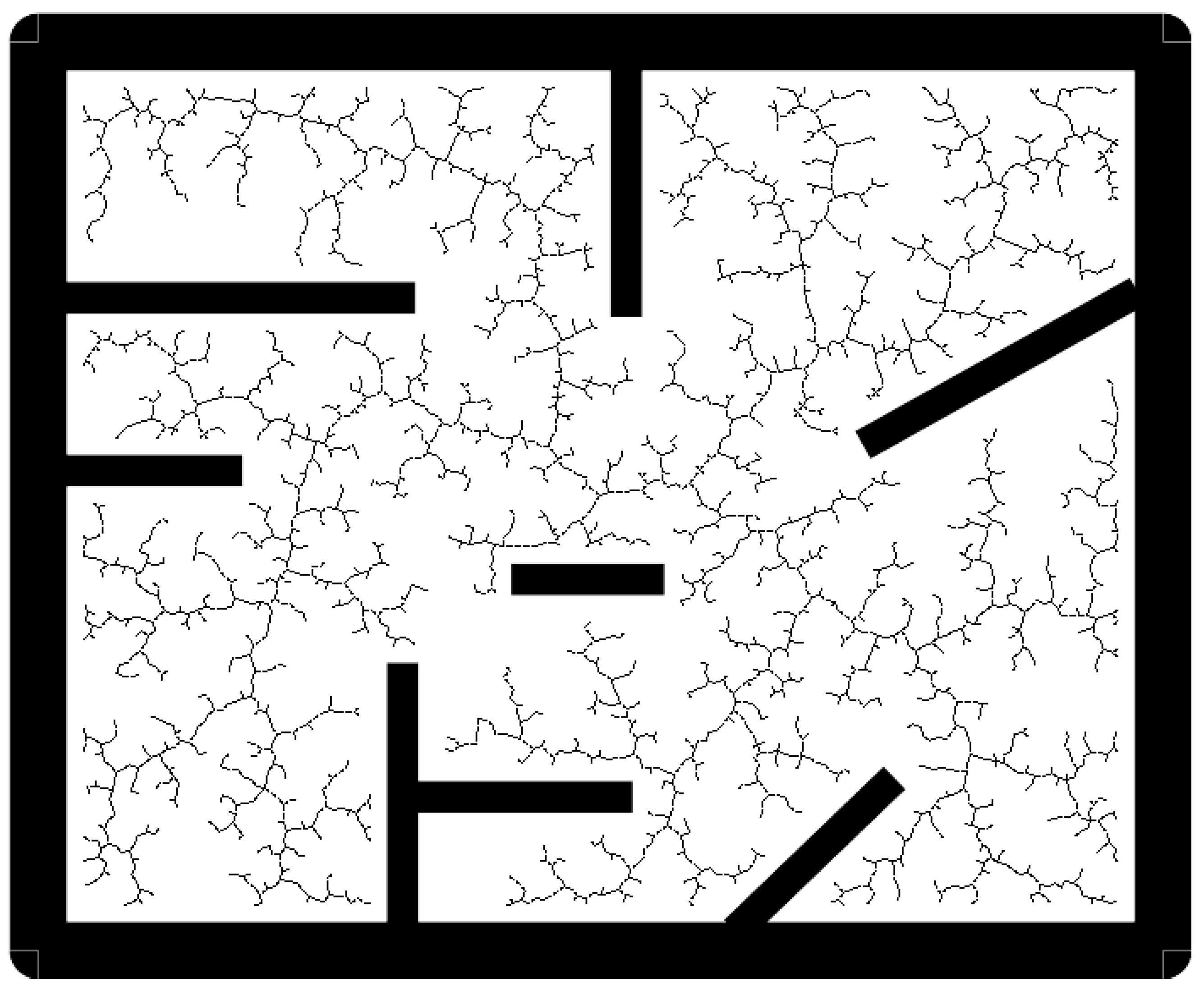
In general terms, the rapidly-exploring random tree (RRT) algorithm builds an exploration tree for a motion planning problem, where the root is the initial state, and each node in the tree represents a reachable state. Thus, each edge in the tree represents a motion connecting two states. Leaf nodes represent final states; when a leaf node reaches the goal area for the motion planning problem, then the trajectory can be generated by connecting the motions (edges) from the root to the leaf node. As a randomized planning technique, the RRT has several good qualities such as being biased to an unexplored state space, the nodes (referred to as RRT points in this paper) being nearly uniformly distributed, only nearest-neighbor queries being needed, etc. The RRT has been increasingly applied in path planning since its establishment in 1998 [5,6]. To compute the $(n+1)$th ($n\ge 2$, initial point is included) RRT point, there are n distances between RRT points and the random point to be computed. The size of the subsequent compare logic determining the nearest distance would also be large if n was a large number. In addition, its size would keep increasing if more RRT points were required. This is a incremental process; so, the RRT belongs to the category of incremental sampling-based motion planning algorithms. If m denotes the number of obstacle points, in the verification process of each iteration, m distances of obstacle points to the line segment $(x_n,y_n)-(x_{new},y_{new})$ should be computed and the nearest distance should be chosen, compared with the robot rotation radius $\xi$ to determine whether to discard or store the potential point $(x_{new},y_{new})$. If the nearest distance is smaller than $\xi$, when the robot walks along this line segment, it bumps into obstacles. So, only when the nearest distance is larger than $\xi$ can the potential RRT point be accepted.

The procedures of determining the nearest RRT point to a random point and the verification process can be performed in parallel. The processing speed will be improved to a large extent if these computations are executed in parallel hardware architecture. To this aim, this research models the RRT algorithm in a GNPS and implements this model on an FPGA. The IEEE 754 floating point number is selected as the real number format for its large dynamic range and high precision. This format allows the future application of the RRT into a large-scale map with a number of obstacle points.

The issues of the FPGA implementation of a GNPS consist of: (1) the mapping between the membrane structures and the hardware description language constructs; (2) the manipulation of the sequential computing associated with different membranes; (3) the realization of parallel computing within one membrane of a GNPS when implementing it on an FPGA. The problems of the FPGA implementation of the RRT algorithm include: (1) after the nth RRT point is generated, to compute the potential (n + 1)th RRT point, there are n distances among RRT points and the (n + 1)th random point to calculate. Note that this is an accumulating computation. Namely, the number of distance calculations above accumulates along with the number of RRT points. How can such accumulating computations be performed? (2) To evaluate the the potential (n + 1)th RRT point, the distances between all the obstacle points and the potential RRT point should be calculated concurrently. These computations are carried out in each round of computing RRT points. In practice, the number of obstacle points is a large number (thousands of thousands). How can these computations be executed properly? (3) It is comparatively easy to generate pseudo random numbers based on a linear shift feedback register. However, if a floating point format is used, generating a floating point number in the range of $(0,1)$ is not trivial. A novel method should be proposed.

To address the issues mentioned above, we conceived corresponding solutions. For issues of the FPGA implementation of a GNPS: (1) Membrane structures are mapped to Verilog modules. The inclusion of membranes is identically transferred to associated modules; (2) The group of computations inside different membranes is triggered by sequential binary impulses; so, the sequential computing of the RRT algorithm is achieved; (3) The group of computations inside the same membrane is triggered by one binary impulse; so, the parallel computations take place correctly. For issues of the FPGA implementation of the RRT algorithm: (1) If the n RRT point will be computed, n distance computing modules (DCMs) are instantiated at first. However, only the right number of DCMs are activated and under use to calculate the corresponding number of distances in a different round; (2) If the number of obstacle points is m, then m DCMs are instantiated under the circumstance that the FPGA hardware resources are sufficient. These DCMs are triggered at the same time to perform parallel computing; (3) Two linear feedback shift registers (LFSR) are chained in order to increase the randomness. These two LFSRs produce 27-bit random numbers. The highest five bits ‘0_0111’ are concatenated at left to the 27-bit number to form a 32-bit number in the range of $(0,1)$.

The proposed FPGA architecture for the RRT algorithm is a novel one because the one membrane computing model, i.e., the GNPS, is utilized as the modeling framework to rebuild this algorithm. Sequential computations are accommodated in different membranes numbered from two (membrane one is the skin to hold all the inner membranes) to the last one. Parallel computations triggered by the same binary impulse reside in one membrane. The employment of the GNPS results in the RRT algorithm being structured and flattened: the computations commence from membrane two sequentially, while the computations within one membrane are carried out in parallel. The advantages of this reconstruction lie in the following: (1) The modularization of the RRT algorithm is beneficial to understanding how this complicated algorithm works; (2) It is quite favorable for FPGA implementation, since the membrane structures are mapped to Verilog module interconnections; (3) This architecture has good scalability. For different maps with different numbers of obstacles and the number of RRT points to be computed, instantiating different numbers of distance computing modules can meet specific requirements. The penalties of this architecture consist of the following: (1) The basic knowledge of membrane computing is indispensable. This precondition may be a barrier for applications of this architecture; (2) FPGA hardware resource expenditure and power consumption are relatively higher for the use of a floating point format. So, this architecture is not suitable for mobile applications powered by batteries.

This architecture was validated in a map containing eight obstacle points, and two RRT points were generated. Although the numbers of obstacle points and RRT points were small, it is easy to scale this architecture by instantiating more or fewer distance computing modules. Compared with the software simulation of this GNPS–RRT model, the GNPS–RRT FPGA architecture achieved a speedup of ${10}^4$ order. The speedup indicates that this architecture has good performance, which can be used to accelerate the RRT algorithm. Furthermore, this study shows that modeling computation intensive algorithms with a GNPS is a feasible and favorable alternative. By means of this rebuilding and modeling of algorithms, FPGA implementation-friendly models are obtained. This study may provide a typical case for modeling with a GNPS and its FPGA implementation, which will expand applications of membrane computing.

The contributions of this study consist of the following: (1) A GNPS is employed as the modeling framework for the RRT algorithm, providing an alternative way to structure computation intensive algorithms; (2) The GNPS–RRT model is desirable for devising a new FPGA architecture, which exhibits feasibility and efficiency. This attempt expands the hardware implementation research of a GNPS and its application; (3) The GNPS–RRT FPGA architecture works with the IEEE 754 floating point format. An original method to generate floating point numbers in the range of $(0,1)$ is proposed.

The paper is organized as follows. Section 2 gives a short introduction to the model of generalized numerical P systems, to RRT algorithm functioning, and to floating point numbers’ representation in hardware. In Section 3, the pros and cons of the existing hardware implementations of the RRT algorithm are analyzed. Section 4 presents the GNPS implementations of the RRT algorithm and its FPGA implementation. Section 5 gives the obtained experimental results and their analyses. Section 6 concludes this paper and discusses the strong and weak points of the proposed implementation.

2. Preliminaries

In this section, the definition of a GNPS is given, and this computing device is represented in detail, so that readers outside membrane computing can understand it well. The RRT algorithm is also explained to reveal the characteristics and computations involved. A brief introduction to the IEEE 754 floating point format is presented at the end of this section. Section 2.1 describes the GNPS, while Section 2.2 gives a detailed description of the RRT algorithm. Section 2.3 displays the IEEE 754 format explicitly.

2.1. Generalized Numerical P Systems

The main model used in this paper is called a generalized numerical P system (GNPS) [4]. It extends a simpler model called a numerical P system (NPS), introduced in 2006 [2] to model economic processes. The model structure of a GNPS corresponds to a graph where each node, called a cell or also a membrane, contains a set of real-valued variables. Some variables are marked as input variables and are read-only (cannot be updated by the rules of the system), while others are marked as output variables and are write-only (cannot be read by the system). All other variables are called internal variables. The model also contains a set of rules that allow updating the values of variables based on their values at the previous discrete time step. The application of rules is guarded by (recursive) predicates, and theoretically, they can perform any transformation. It should be noted that a locality principle is used—any transformation may only consider values of variables located in the same cell.

For implementation reasons, it is often interesting to use integer variables and linear predicates and transformations. This allows achieving very high implementation speeds. The basic variant of a GNPS corresponds to such a restriction, enriched with explicitly mentioned nonlinear functions that can be additionally used.

We provide the formal definition of a GNPS as well as its semantics, as follows [4,7].

Definition 1. 

A generalized numerical P system is the following tuple

$$\mathsf{\Pi }=(m,V,I,O,(Va{r}_1,Va{r}_1\left(0\right)),\dots ,(Va{r}_m,Va{r}_m\left(0\right)),Pr),$$

where

• $m>0$ is the number of cells/membranes,
• V is an alphabet of variables,
• $I\subseteq V$ is the set of input variables, $I\cap O=\varnothing$,
• $O\subseteq V$ is the set of output variables, $I\cap O=\varnothing$,
• $Va{r}_i\subseteq V$ is the list of internal variables for cell i,
• $Va{r}_i\left(0\right)$ is the vector of initial values for variables internal to cell i,
• $Pr$ is the set of rules of the system (see the description below).

A rule (called also program) $r\in Pr$ has the following form

$$\begin{array}{cc}\hfill & P(x_{1i},\dots ,x_{ki};E_1,\dots ,E_l);\hfill \\ \hfill & F(x_{1i},\dots ,x_{ki})\to c_1|v_1,\dots ,c_n|v_n,\hfill \end{array}$$

(1)

where

• $\{x_{1i},\dots ,x_{ki}\}\subseteq Va{r}_i$ for some i, $1\le i\le m$, are variables located altogether in the same cell i,
• $\{E_1,\dots ,E_l\}\cap Va{r}_i=\varnothing$ are predicate variables located in cell i above,
• $\{v_1,\dots ,v_n\}\subseteq V$ are any variables of the system,
• $c_j\in \mathbb{N}$, $1\le j\le n$ are repartition coefficients that together with variables $v_j$ form the repartition protocol,
• P is the applicability condition, which is a decidable predicate over the indicated variables,
• F is the production function, which is a computable function.

In the definition above, the values of the variables are considered to be real. Then, it is clear that the predicate P should be decidable, and the function F should be computable on real numbers. Since, from a theoretical point of view, most of the predicates on real numbers are undecidable, in this paper we understand by “decidable on reals” any predicate decidable on a chosen representation (approximation) of real numbers. Similarly, the computability on real numbers refers to the computability using the chosen representation of real numbers. In the case of an always true predicate, it can be omitted.

Since each variable has a unique cell to which it belongs, the rules in $Pr$ can be interpreted as the structural relation between cells to which the involved variables belong. In the most general case, this relation induces a hypergraph; however, special cases of graph and tree relations are of particular interest for membrane computing. In the latter case, the system can be depicted graphically as a Venn diagram, where the variables and rules are located in corresponding cells.

In order to apply a rule r as described above, first, its applicability condition is checked. If predicate P is true, then the rule is called applicable, and it is applied as follows [2,4,7]. First the value of the production function is computed, based on the current values of the variables. Second, each variable $v_j$, $1\le j\le n$ from the repartition protocol part receives the fraction $\frac{c_j}{{\sum }_{t=1}^n{c}_t}$ of the computed production function value. If there are several applicable rules, then all of them are applied. If several rules update the same variable, then the corresponding amounts are added. Finally, the value of a variable at the beginning of each new step is reset to 0 if it was used in a computation of some production function. The value of an output variable is always kept to the previous value, unless updated. In this case, the old value is replaced by the newly computed value.

The evolution of a GNPS can be described by the following discrete time series (we suppose that r is described as in (2)):

$$x_{ls}(t+1)=\sum _{r\in Pr}F\left(x_{1i}\left(t\right),\dots ,x_{ki}\left(t\right)\right)\frac{c_j}{{\sum }_{t=1}^n{c}_t}+{\overline{x}}_{ls}\left(t\right),$$

(2)

where ${\overline{x}}_{ls}\left(t\right)=\left\{\begin{array}{cc}{x}_{ls}\left(t\right)\hfill & \mathrm{if}{x}_{ls}\mathrm{does}\mathrm{not}\mathrm{appear}\mathrm{in}\mathrm{any}\hfill \\ & \mathrm{production}\mathrm{function}F\mathrm{of}\mathrm{an}\hfill \\ & \mathrm{applicable}\mathrm{rule},\hfill \\ 0\hfill & \mathrm{otherwise}.\hfill \end{array}\right.$

We recall that the initial values (at time 0) of variables from cell i are given by the set $Va{r}_i\left(0\right)$.

2.2. The Rapidly-Exploring Random Tree (RRT) Algorithm

The pseudo code of the RRT algorithm is given in Algorithm 1. In general terms, the RRT algorithm builds an exploration tree for a motion planning problem, where the root is the initial state, and each node in the tree represents a reachable state. Thus, each edge in the tree represents a motion connecting two states. Leaf nodes represent the final states; when a leaf node reaches the goal area for the motion planning problem, then the trajectory can be generated by connecting the motions (edges) from the root to the leaf node (Figure 1).

Algorithm 1: Pseudocode for the RRT algorithm.

Input: Initial position: $X_0=(x_0,y_0)$, size of RRT: N, step: $\delta$, radius: $\xi$, list of obstacle points: L     Output: RRT Graph: G 1  Add vertex $X_0$ to G 2  for $i=1$to N do$\phantom{(}$ 3         $X_{rand}\leftarrow$ random point on the map 4         $X_{near}\leftarrow$ nearest vertex from G to $X_{rand}$ 5         $X_{new}\leftarrow$ point situated at distance $\delta$ from $X_{near}$ when moving towards $X_{rand}$ 6         if $\exists p\in L$ with the distance between p and $X_{near}{X}_{new}<\xi$, then 7                go to step 3 8         Add vertex $X_{new}$ to G 9         Add edge $(X_{near},X_{new})$ to G

At the beginning of the RRT algorithm, the first random point $(x_{r{d}_1},y_{r{d}_1})$ is produced as $(p\times rd{m}_1,q\times rd{m}_2)$, where p and q are the x-axis length and y-axis height of the map. $rd{m}_1$ and $rd{m}_2$ are two random numbers in the range of $(0,1)$. The initial position of the robot, which is also the root point of the RRT, is $(x_1,y_1)$. On the line segment $(x_1,y_1)-(x_{r{d}_1},y_{r{d}_1})$, a shorter one, whose starting point is $(x_1,y_1)$ and length is $\delta$, is computed. $\delta$ is called the step length of the RRT path. If the distance of $(x_1,y_1)-(x_{r{d}_1},y_{r{d}_1})$ is less than that of $\delta$, then $rd{m}_1$ and $rd{m}_2$ are regenerated until $|(x_1,y_1)-(x_{r{d}_1},y_{r{d}_1})|\ge \delta$. If we find such a line segment whose length is $\delta$, then the end point of this line segment $(x_{ne{w}_1},y_{ne{w}_1})$ is the first potential RRT point. To verify this point, the distances among all obstacle points to the line segment $((x_1,y_1)-(x_{ne{w}_1},y_{ne{w}_1}))$ are calculated in parallel. Then, the minimum distance is determined by comparing these distances pairwise. If the minimum distance is larger than the robot rotation radius $\xi$, then $(x_{ne{w}_1},y_{ne{w}_1})$ is recognized as the second RRT point $(x_2,y_2)$ (note that the root RRT point, which is the initial position of the robot, is $(x_1,y_1)$). Otherwise, $(x_{ne{w}_1},y_{ne{w}_1})$ is discarded, and $(x_{r{d}_1},y_{r{d}_1})$ is recomputed until $(x_1,y_1)$ is obtained.

To acquire $(x_3,y_3)$ is more complicated. Once the second random number $(x_{r{d}_2},y_{r{d}_2})$ is computed, we should compare the length of line segment $(x_1,y_1)-(x_{r{d}_2},y_{r{d}_2})$ and $(x_2,y_2)-(x_{r{d}_2},y_{r{d}_2})$, choosing the minimum one. Then, we calculate the line segment whose length is $\delta$ on the minimum one if its length is equal or larger than $\delta$. As mentioned above, the endpoint $(x_{ne{w}_2},y_{ne{w}_2}$ is the second potential RRT point. To confirm it, the distances among all obstacle points to the line segment $((x_{s{p}_1},y_{s{p}_1})-(x_{ne{w}_2},y_{ne{w}_2}))$ are calculated in parallel, where $(x_{s{p}_1},y_{s{p}_1})$ is $(x_1,y_1)$ or $(x_2,y_2)$. As can be seen, the process computing an RRT point comprises two phases. In the first phase, there is an accumulating distance calculation that determines the minimum distance to the random point. Specifically, to compute the $(n+1)$th RRT point ($(x_1,y_1)$ is included), there are n distances to compute; and the minimum one is selected by pairwise comparison. The second phase is the verification involving the calculation of distances among all obstacle points to the target line segment. This phase is static because the number of obstacle points is constant.

2.3. Real Number Representation

We would like to remark that the model of a GNPS considers real-valued variables. Note that real numbers are represented by their approximation using bit arrays. There exist two main possibilities for such a representation: fixed point and floating point formats.

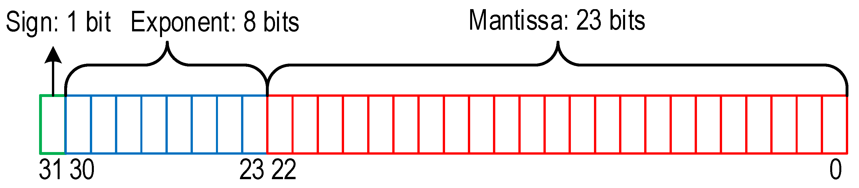
The usage of fixed point encoding in the implementation presents many benefits; however, it has a major drawback—its dynamic range is relatively small. This can be penalizing for several types of applications, including the RRT algorithm. To increase it, a larger number of bits for the representation should be considered, even if most of the possible values would remain unused. If the limit values cannot be determined in advance, then there is an important risk of overflow. The floating point representation of (the approximation of) real numbers aims to deliver a large dynamic range, while trading off the number precision. The most common format for such a representation is the IEEE 754 single precision floating point format, depicted in Figure 2. As can be seen, the total size of the representation is 32 bits. Bits 0 to 22 store the mantissa, and bits 23 to 30 store the exponent of the number. The last bit denotes the sign, 0 for positive and 1 for negative values. The exponent is an 8-bit unsigned integer in a biased form: an exponent value of 127 actually represents 0. Additionally, the exponents range from −126 to +127 because the exponents of −127 (all 0 s) and +128 (all 1 s) are reserved for special numbers.

3. Related Works

The development of robots able to act in real-world environments implies the study and research of anytime algorithms, i.e., algorithms able to return a valid solution to a problem even if they are interrupted. In the particular case of mobile robots, one crucial problem to be solved by this type of algorithm is the motion planning problem. This problem demands finding a sequence of commands that allow moving an agent from an initial state (usually a position in a 2D plane) to a final one, while avoiding obstacles [8]. In [9], the mentioned problem is demonstrated to be PSPACE-hard. Therefore, several approximated solutions have been designed. One special case is the category of algorithms to build Rapidly-exploring Random Trees (RRTs). They are based on a randomized exploration of the obstacle-free configuration space by creating a data tree structure in which the nodes represent reachable states and the edges represent transitions or movements between states. Several variants of the main algorithm have been designed, in particular, the RRT${}^{*}$ algorithm [10] is able to create a tree whose branches asymptotically converge in computation time to optimal solutions.

Attempts to speed up the execution of the RRT algorithm led to the investigation of its parallelization strategies. While the main core of the RRT algorithm is iterative and, therefore, sequential, there are parts that have been successfully implemented on parallel hardware in the obstacle collision detection [11,12]. Another possibility is to use an inherently parallel model of computation such as membrane computing [1] to encode the algorithm. Then, a parallel implementation of the corresponding model would result in a parallel RRT solution.

In recent years, several hardware implementations of the RRT algorithm have been developed by using custom FPGA hardware [13,14], by using CUDA GPUs [15,16], and by using the OpenMP platform [16]. In particular, in [13], a hierarchical FPGA architecture was proposed to speed up the RRT algorithm. In this architecture, multiple RRT modules were executed concurrently to obtain their results. These results were integrated to form the path via a write-access mechanism. In detail, after a potential RRT point (called as ‘node’) was calculated by a RRT module, this point was polled. If it was acknowledged as a node by the polling module, it was transferred to generate the global path. Otherwise, a new iteration began to compute the potential node. The polling module is a buffer stack storing nodes. To preserve data integrity, all the nodes are transferred through a write-acknowledge mechanism. A FIFO stack is configured to poll those polling modules in a chronological sequence. Polling modules send data to the FIFOs after receiving the instant read access request sent by the latter. There are several FIFO polling levels in which the higher levels poll the lower ones. A global map module, located at the top of the polling tree, is updated by its immediate lower FIFOs.

The benefits of this architecture consist of the following: (1) The polling tasks only come from the immediate higher levels so that the data integrity is preserved. Consequently, zero intra-level communication is achieved; (2) Data collision is avoided, where data scheduling happens only among the immediate lower modules. As the result, the waiting time is reduced to a large extent; (3) The number of each kind of modules can be adjusted, for the depth of the hierarchical structure. However, the limitations include the following: (1) Except for the global map module, most parts inside each module are reusable in different iterations. Nevertheless, they are instantiated many times, consuming a lot of hardware resources. So this strategy incurs more power consumption; (2) The map should be described by obstacle points instead of the real map picture for an FPGA. So, the number of obstacle points of each map should be determined. This number is important because it decides how many distance computations are conducted in the polling process. If the number of the RRT module is lower than the number of obstacle points, what will they do? Can they compute the distance in several rounds, or there is another solution? (3) The relative performance proposed is not suitable for evaluating the performance of this architecture. The absolute performance (the concrete time elapsed to plan a path from initial position to destination) is more acceptable. Another weak point is that the hardware resource consumption is not mentioned.

Compared with the existing FPGA implementations mentioned above, the FPGA architecture proposed in this paper has the following advantages: (1) Floating point arithmetic units are instantiated in one instance to reduce the hardware expenditure and power consumption; (2) A target map is described with obstacle points and the length × width. The number of obstacle points is clear-cut and constant. This fact benefits the implementation of the RRT; (3) The absolute performance is employed to evaluate our architecture. The hardware expenditure and power consumption of our design are provided as well, which are necessary to assess this architecture. The disadvantages of our architectures lie in the following: (1) the floating point format consumes many more hardware resources than the fixed point format, although the former has a much larger range and higher precision; (2) For the limited hardware resources of an FPGA, it is almost impossible to instantiate enough distance computing units to calculate the distances simultaneously. A mechanism which arranges the distance computing in sequential batches is needed. This mechanism will be investigated in the next phase.

4. Methods

In this section, the design and implementation of the FPGA architecture for the GNPS-modeled RRT algorithm are elaborated. We describe the modeling of the RRT algorithm with a GNPS in Section 4.1. As a consequence, a GNPS computing RRT points is obtained. This GNPS is used as the roadmap for the FPGA architecture design. In Section 4.2, the design of the associated floating point arithmetic units working as functional parts of FPGA architecture is described. In Section 4.3, the implementation of this architecture is presented.

4.1. GNPS Modeling of the RRT Algorithm

The modeling of the RRT algorithm using a GNPS closely follows Algorithm 1 and performs parallel operations whenever possible. The state space corresponds to a rectangle of a given size in the 2D plane. The maximum number of RRT points and the number of obstacles are fixed in advance. These values can be changed if necessary. Each obstacle and RRT point is represented by a couple of GNPS variables corresponding to their coordinates. After obtaining the random point $X_{rand}$ using a pseudo-random number generator, distances from this point to all the available RRT points are computed in parallel. Then, the minimum distance is found, the corresponding RRT point is selected as $X_{near}$, and the new candidate RRT point $X_{new}$ is computed. Then, the distances from each obstacle point to the line segment $X_{near}{X}_{new}$ are computed in parallel. If these distances are smaller than the robot rotation radius $\xi$ (there is a collision), the process is reiterated.

The GNPS modeling of the RRT is based on a functional group partition to the algorithm. As a consequence, different functional groups are located in different membranes, while these membranes are enclosed by a skin membrane, composing the GNPS as a whole. From the coarse-grained point of view, procedures computing $X_{rand}$, $X_{near}$, and $X_{new}$ can be regarded as a functional group, contained in an internal membrane. Note that these procedures are executed serially for the implicit sequence. 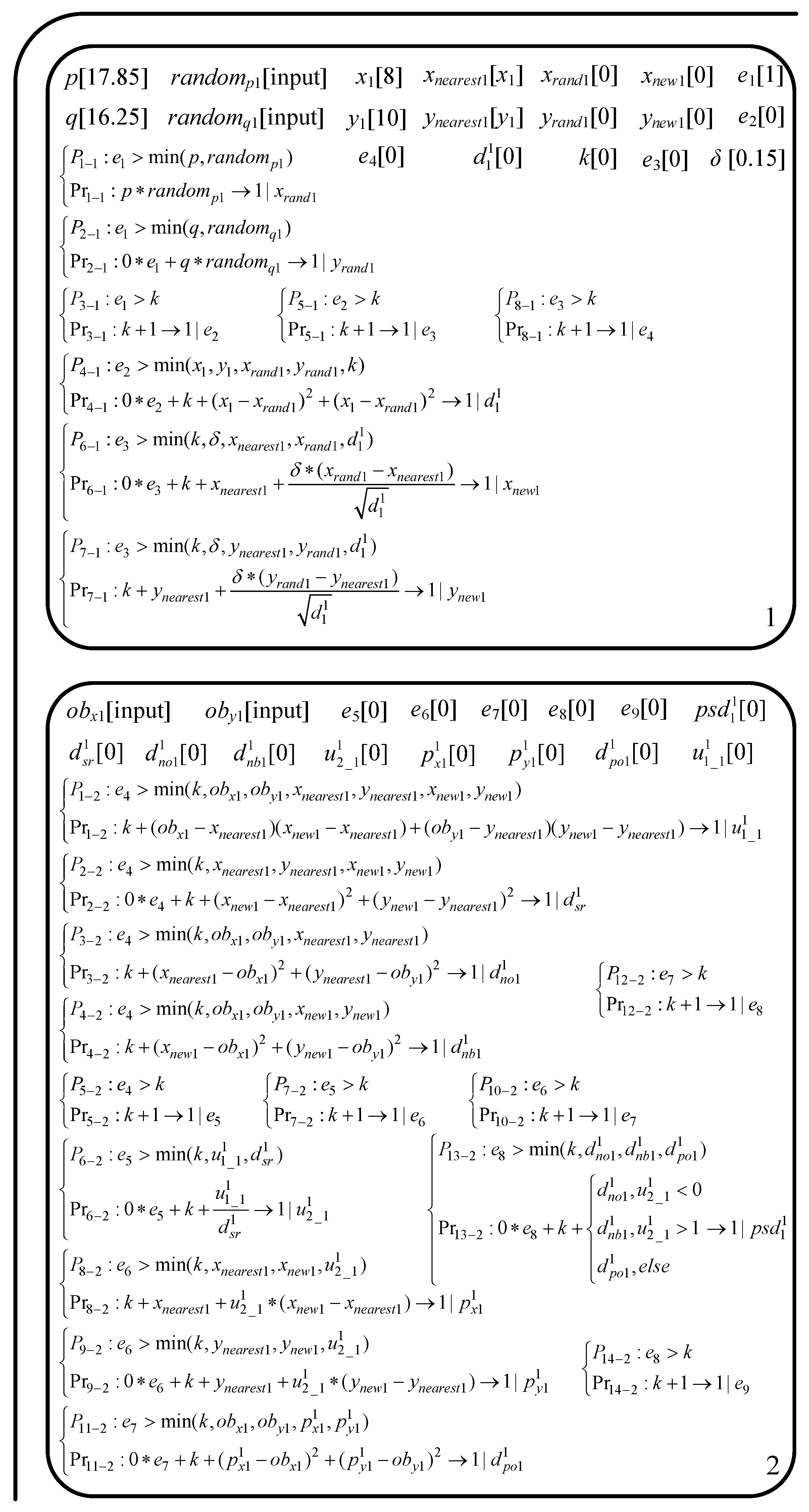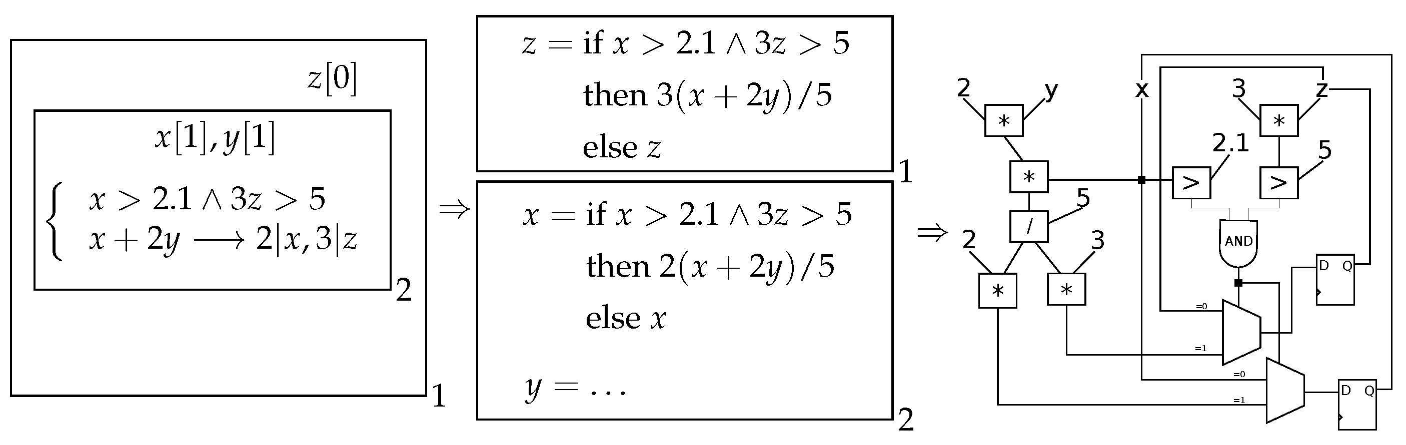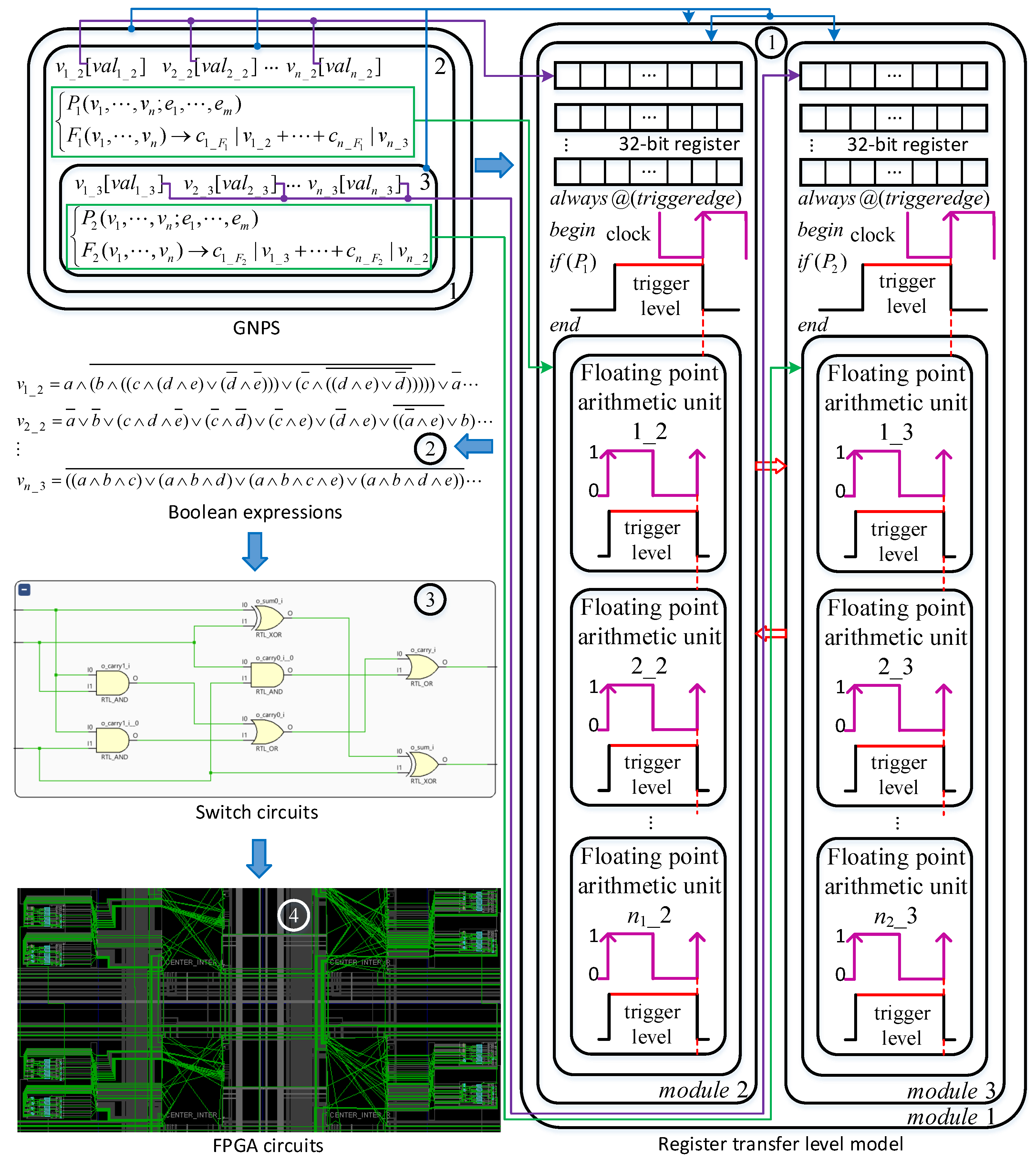The calculations of the distances from the obstacles to $X_{near}{X}_{new}$ can be conducted in parallel, although they have sequential procedures. Such a calculation is treated as a functional group; so, they reside in multiple membranes. The number of these membranes is equal to the number of obstacle points. Finally, the process of choosing the minimum distance and verification is another functional group split into fine-grained view to organize the distance comparison. The membrane groups standing for these three functional groups execute serially to conform to the RRT algorithm, while the applicable programs in all these membrane are performed in parallel. An example of the translation is depicted in Figure 3, where the model is computing the third RRT point in a map having three RRTs and eight obstacle points. The system was built incrementally, first providing the rules for the high-level algorithm description and then refining in subsequent steps by adding new or modifying existing rules.

4.2. Floating Point Arithmetic Module Design

For formulas operating fixed point numbers, Verilog operators can be used. However, to perform arithmetic operations involving IEEE 754 numbers on an FPGA, one should use floating point arithmetic units (FtPAUs) because the Verilog arithmetic operators are only compatible for fixed point numbers. The execution of the arithmetic operations is inherently sequential: operations with higher priorities, such as multiplication and division, should be performed ahead of operations with lower priorities, such as addition and subtraction; operations with the same priority are executed serially. Hence, to conduct a production function of a GNPS program operating floating point numbers, several FtPAUs will be chained in a specific order to form a FtPAU group to perform the calculation correctly. To this end, a trigger signal is indispensable to fire the associated FtPAUs sequentially. On the other hand, the FtPAU groups corresponding to all applicable programs should be triggered simultaneously to comply with the parallelism, while the nonapplicable programs’ FtPAU groups cannot be fired. Here, trigger signals are needed again.

For a GNPS working with fixed point numbers, predicates are translated to logical expressions and employed as the conditions of if–else statements of Verilog language. Production functions comprised with Verilog arithmetic operators and variables reside in these statements, acting in line with the results of these logical expressions. Nevertheless, in hardware description language (HDL) development, instantiated FtPAU groups cannot be placed in such constructs. The treatment of predicates in a fixed point scenario should be changed in a way that adapts to the new form of programs. In our research, the function of logical expressions representing predicates is substituted by trigger signals with equivalent functions.

FPGA vendors provide basic FtPAU intellectual property (IP) cores: an adder, a multiplier, and a divider. These FtPAUs are triggered by the rising edge of the clock. This is a general setting but not suitable for constructing complex computations such as the RRT algorithm. FtPAUs that are triggered at different times and hold their values after computing are more preferred. The main reason is that developers should schedule all the calculations to implement the algorithm correctly. FtPAUs triggered at the clock rising edge actuate at the same time, keeping developers from utilizing distinct FtPAUs, resulting in the chaotic timing of computations. Following this idea, associated FtPAUs are developed to have different trigger conditions. FtPAU IP cores are not used except for the normal divider, which is a long time-latency and high resource-expenditure FtPAU. The following IEEE 754 compliant arithmetic units were designed: an adder, a multiplier, and an inverse square root. The comparator and pseudo-random number generator were also devised to fulfill the demand.

Our implementation of the FtPAUs triggered them sequentially for a single group of operations. To implement this, it used input state and output control signals (wires/bit variables). The first signal allowed the activation of the unit when the signal was asserted high (equal to one). After the end of the computation (which may take several clock cycles), the high control signal was asserted (during one clock cycle) indicating that the result was computed. The control signal of an unit from a FtPAU chain was connected to the state port of the next one to activate it. For each FtPAU, several implementations were designed targeting different timing setups and computation conventions.

Addition and subtraction were realized by a single unit that takes as input two operands and the operation to perform (+ or −). Since the IEEE 754 representation contains the number sign, the operation of the unit should be handled with care (a subtraction can become an addition, indeed). To reduce hardware resources and power consumption, IEEE 754 exceptions were not taken into account except underflow. Truncation was selected as the rounding mode [17] for the same reason. The design of the floating point multiplier was simpler than the adder, as there was no need to ensure that both numbers had the same exponent.

It was trivial to compare to fixed point numbers since Verilog comparison operators are at hand. However, to compare to floating point numbers was not as straightforward due to the lack of comparison operators. The floating point comparator was designed to conduct the comparison. Since floating point numbers consist of sign, exponent, and mantissa, these parts were compared successively. The RRT algorithm involved the comparison of numbers with the same sign. An absolute value comparison method, which combined the exponent and mantissa was devised, as shown in

Table 1. Comparison of two FP numbers with the same signs.

Sign of a	Sign of b	abs	Output
+	+	$\left|a\right|>\left|b\right|$	b
+	+	$\left|a\right|<\left|b\right|$	a
−	−	$\left|a\right|>\left|b\right|$	a
−	−	$\left|a\right|<\left|b\right|$	b

. Note that the comparator output the smaller number.

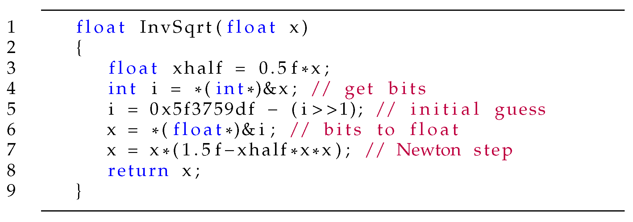
The RRT algorithm involves the inverse square root calculation for new RRT point generation. Instead of attacking the problem directly by performing radication and division, we used an ingenious solution for this problem, which first appeared in the source code of the Quake3 3D game launched in the 1990s, see Figure 4. This solution is based on a Newton approximation; however, it converges to a low error solution only after the first iteration. We refer to [18] for more details and the analysis of this algorithm. We also used the constant ‘5f37_5a86’ for better precision, as suggested in [18]. To translate this algorithm to Verilog, one should bear in mind that a binary number, either in fixed or floating point format, is treated as fixed point number, if the Verilog operators are exerted, while it is considered as a floating point number, if it is input to a FtPAU. As mentioned above, for normal floating point number divisions that cannot be avoided, we used the corresponding IP cores, which were optimized at time, and resource aspects, directly.

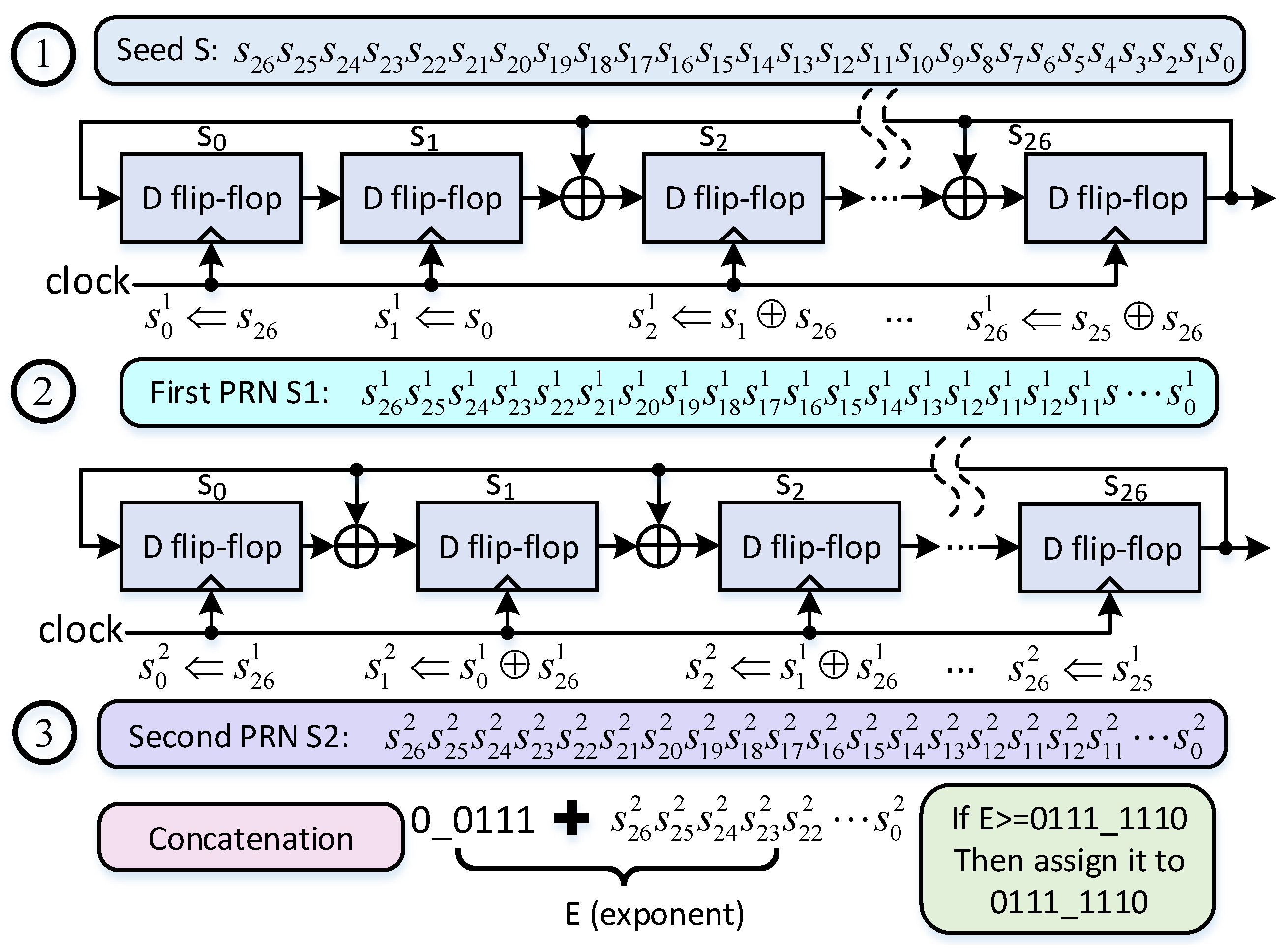
There are two types of random number generators that can be implemented in FPGA: true random number generators (TRNG) and pseudo random number generators (PRNG) [19]. Since it is quite difficult to design a TRNG, we developed a PRNG producing an IEEE 754 floating point number in the range of $(0,1)$. Its construction was based on two chained linear feedback shift registers (LFSR) in order to increase the randomness. It functions in three steps as follows. (1) First a 27-bit seed number is selected. Then, exclusive or (XOR) operations among some bits of this seed are performed yielding the first random number; (2) Next, several exclusive or (XOR) operations among other bits of the first pseudo random number are performed yielding the second pseudo random number; (3) Finally, sequence ‘00111’ is concatenated at the left of the second pseudo random number in order to transform it to a 32-bit IEEE 754 single precision floating number. Finally, the exponent part of this resultant number (denoted by E) is adjusted to be less or equal than ‘01111111’, which is the exponent of the numbers in the range of $(0,1)$. The computation algorithm is shown graphically in Figure 5.

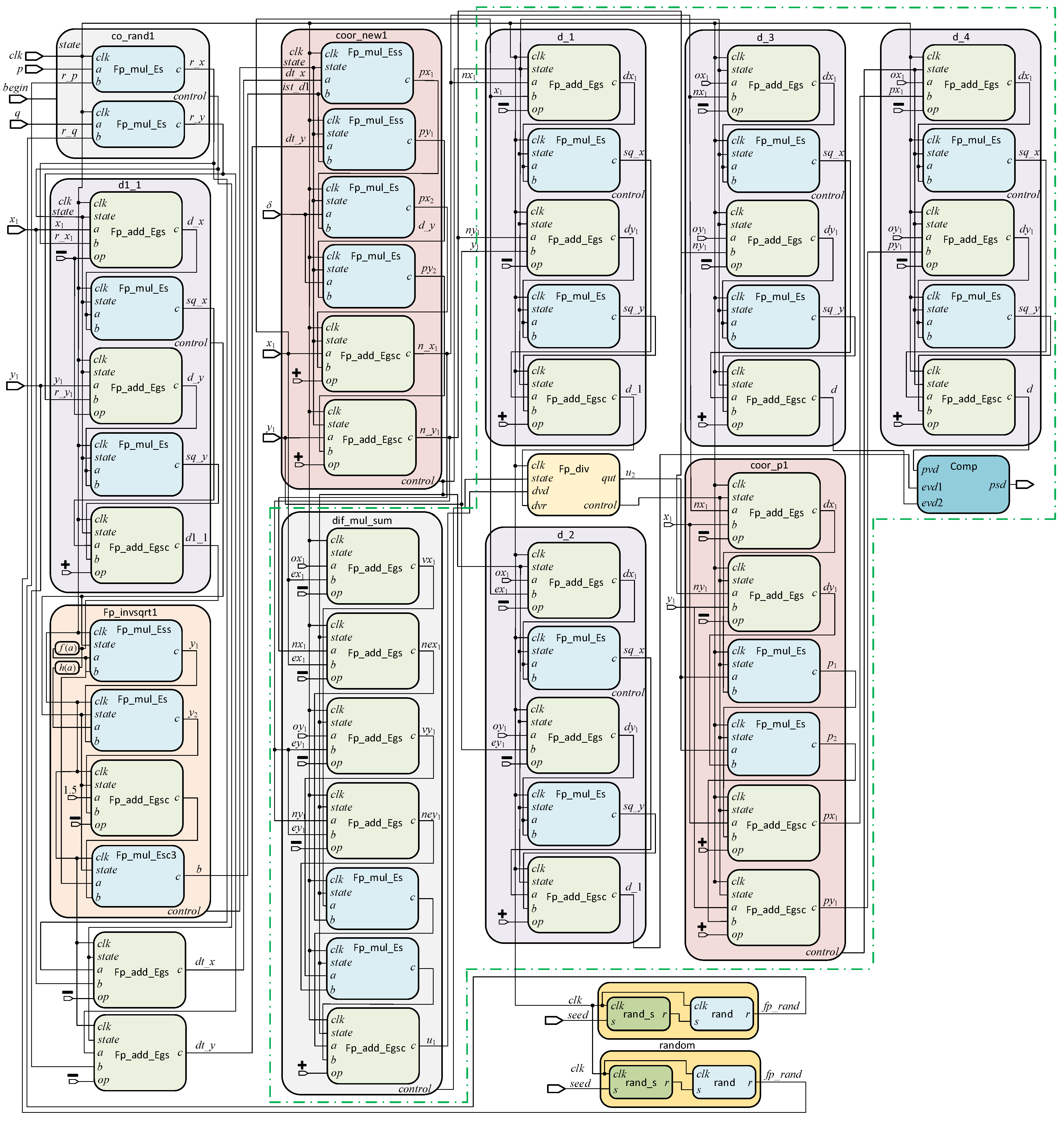
By wiring the corresponding Verilog modules, we can obtain the detailed FPGA architecture of the GNPS-modeled RRT algorithm, which is illustrated in Figure 6. Two random modules depicted at the right bottom provide pseudo random numbers. Module co_rand1 calculates the random point $X_{rand}$. Module d1_1 computes the square distance between initial position and $X_{rand}$ after its generation. Fp_invsqrt1 module computes the inverse square root of this square distance. Two adders adjacent to Fp_invsqrt1 are utilized to calculate the coordinate differences of the initial position and $X_{rand}$. coor_new1 is used to obtain the potential RRT point $X_{new}$. Module dif_mul_sum, d_1, d_2, and d_3 begin to work simultaneously to verify whether or not $X_{new}$ is an RRT point. Module Fp_div is the instantiated divider IP core conducting normal floating point number division. Module coor_p1 obtains the coordinates of the projection of an obstacle point on the line segment. Module d_4 returns the square distance between an obstacle point and its projection. Module Comp selects the proper distance between a point and a line segment for the three distances according to their relative locations.

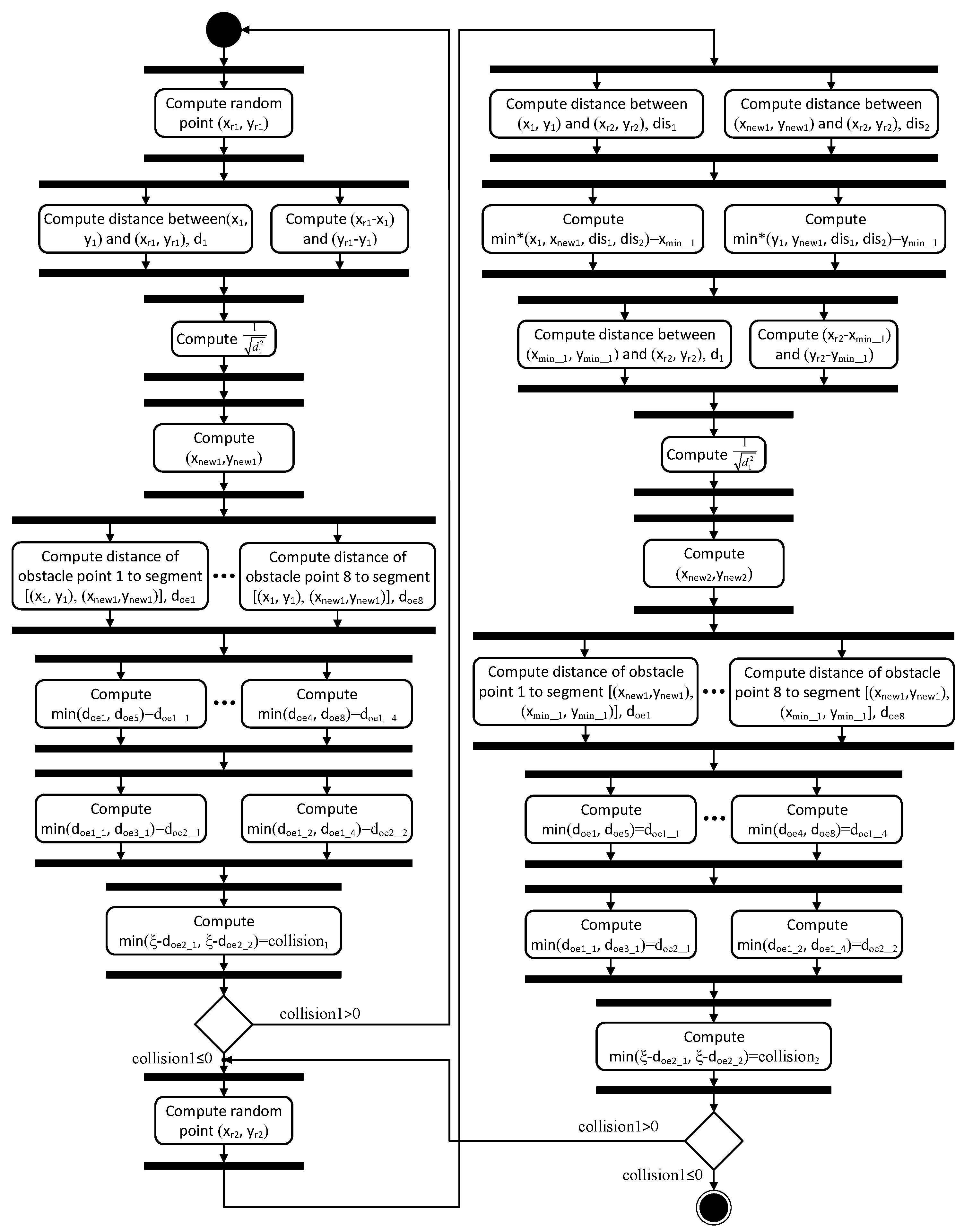
The unified modeling language (UML) activity diagram depicted in Figure 7 details the whole process of the FPGA architecture designed from the GNPS-modeled RRT. It is highlighted that the distances between the obstacle points and the line segment are computed in parallel so the performance will be improved to a large extent. A comparison process is required to determine the minimum distance. This process can be implemented by software.

4.3. FPGA Implementation of GNPS

The FPGA implementation of the GNPS is similar to the method from [4]. First, the target GNPS was rewritten in terms of a time series, as shown in Section 2.1. Next, the obtained equations were translated to Verilog code, yielding an implementation, where all the values of variables for the next step were computed in parallel. However, since the variable values were represented in IEEE 754 format, this translation was not direct as in the case of the fixed point encoding, considered in [4]. To perform the necessary operations, each Verilog module corresponding to a cell/membrane instantiated a number of floating point arithmetic units, whose sequential application yielded the desired result. These units were then wired between each other as well as to the corresponding variables and constants. In order to reduce the latency, the computation was split into several independent parts that were processed in parallel. An overview of the process for a single rule can be seen in Figure 8. The overall computation speed is dependent on the number of independent computational blocs that need to be synchronized [20].

After the design of the RTL model, the implementation phase commenced, which included the following operations: behavioral simulation, synthesis, setting up the debug cores, I/O pins planning, implementation, post-implementation simulation, place and route, and hardware debug. The results computed by the FPGA were probed in the hardware debug to show on screen, with the integrated logic analyzer (ILA) or oscilloscope. In this research, the first one was used for its convenience. The implementation process is diagrammatically shown in Figure 9.

Compared with the method introduced in [13], except for the floating point divider, all the arithmetic modules in this paper were designed from scratch. The inverse square root unit has good efficiency; so, the computation speed was lifted to a large extent. In addition, the trigonometric functions involved were avoided by utilizing this kind of unit. Our paper focuses on designing parallel floating point arithmetic units involved in the RRT algorithm.

5. Experimental Results

To test the described methods, a Xilinx VC707 evaluation board featuring a Virtex-7 XC7VX485T-2FFG1761 FPGA [21] was used. The development and software benchmark tests were performed on a host computer equipped with an Intel Core i7-7820HQ processor and 16 GB RAM. Xilinx Vivado 2019.1 was used as an FPGA integrated developing environment.

The size of the map was a square of 17.85 m, with eight obstacle points. A GNPS computing three RRT points on this map was created and then translated manually to Verilog, according to the procedure described in Section 4. The GNPS consisted of 34 membranes, 220 variables, and 210 rules. The initial position and obstacle points coordinates were read from an external file and stored in the distributed memory of the FPGA. The output was not directly exposed; instead, it was checked during hardware debug by the integrated logic analyzer (ILA). An additional debug core was set together with the synthesized model in order to use the ILA functionality.

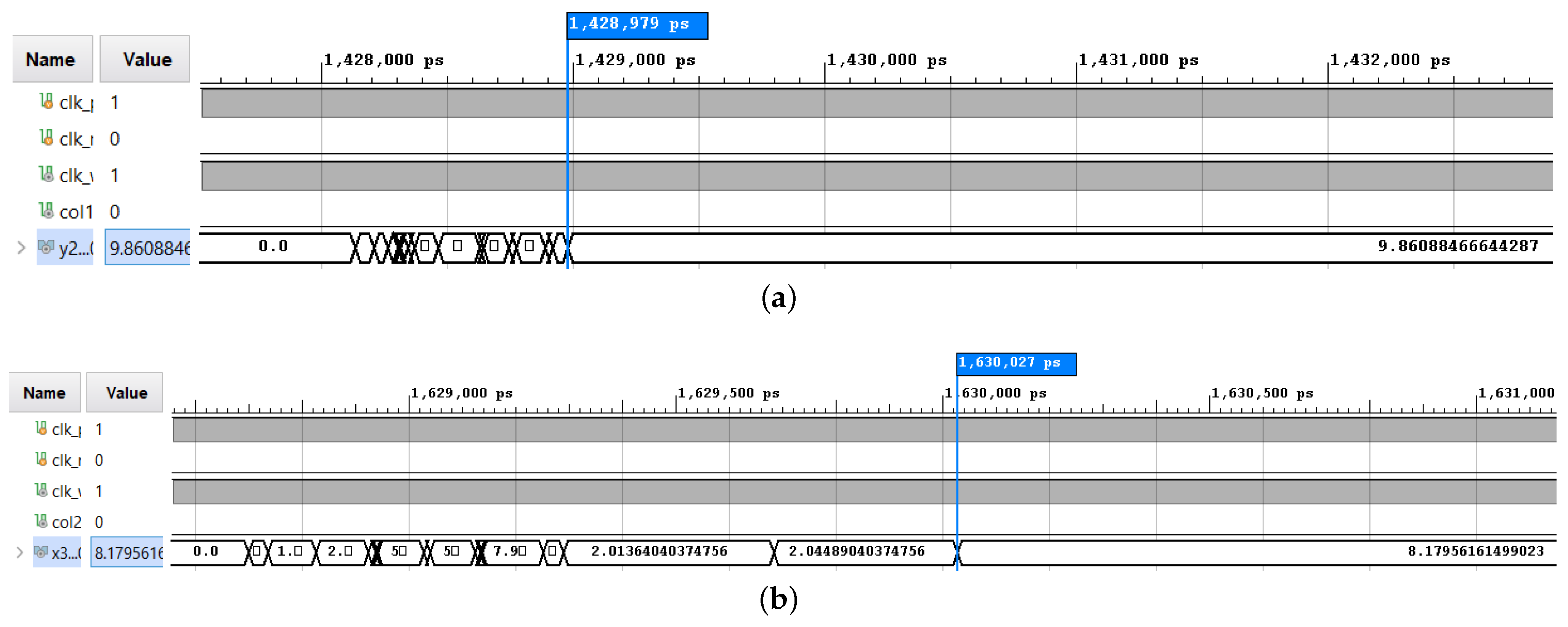
To ensure that the RTL description of a GNPS-modeled RRT algorithm behaved as expected, a testbench was designed, and a behavioral simulation of the design was performed. It confirmed the good functioning of the translation. After the synthesis and the place and route step, we verified that the design met the timing constraints. The clock speed was set to 40 ns (25 MHz) in order to meet them. Next, a post implementation timing simulation was performed. 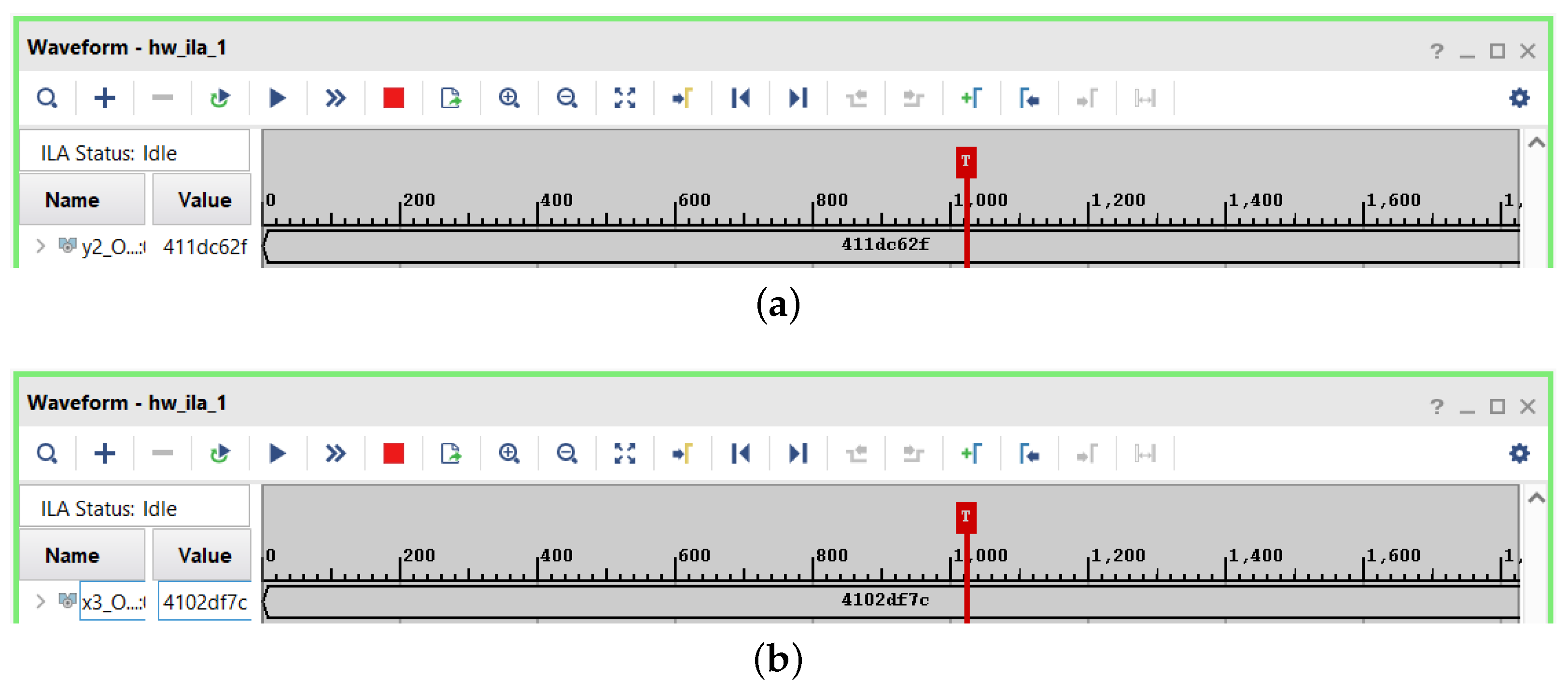This simulation was very similar to a behavioral simulation, but it was time accurate; so, an estimation of the running time was obtained from it, as given in Figure 10. After several post-simulation tests, we determined that it took an average of 3059.01 ns to compute the three RRT points. Next, the design was run on the FPGA hardware. By reading the results using ILA (directly on the hardware), we observed that they corresponded exactly to the values obtained during the post-timing simulation, as shown in Figure 11. Moreover, we would like to note that the obtained time corresponded only to the raw time used by the device for the computation and did not take into account the input/output latency, which is standard practice in the area of the FPGA design. Finally, we remark that we used the same seed for the random number generator for the simulation and the actual run; so, the obtained values were the same.

The software simulation of the same GNPS model was performed by the PeP NPS simulator [22]. This is a straight simulator written in Python that does not use any particular parallelization optimizations. The running time took an average of 0.097948 s to obtain the same results, as shown in Figure 12. The results of the PeP saved two significant digits. When we did the same to the FPGA outcomes, the same numbers were obtained. As in the FPGA case, only the computation part was considered, ignoring the delays induced by the input and the output. So, the obtained speedup was of the order $3.20195\times {10}^4$. We would like to note that by using the basic parallelization techniques, it would be possible to have a faster execution of the PeP simulator; however, this would not change the order of magnitude for the speedup.

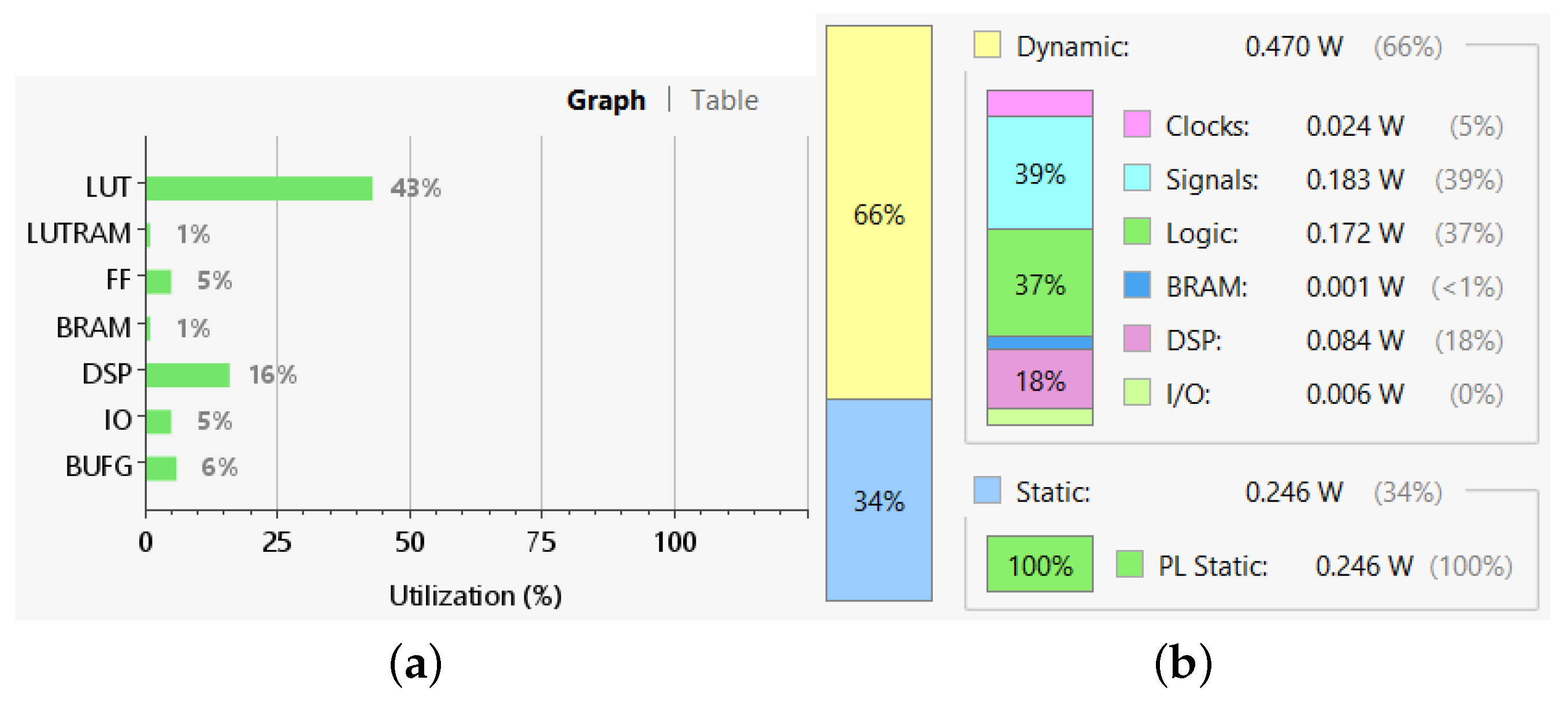
The resource utilization and power consumption of the RRT–GNPS are shown in Figure 13. They were computed automatically by Xilinx Vivado software based on the synthesized design during the post-implementation stage. The implementation used 43% of the look-up table (LUT) resources because of the long 32-bit width of the IEEE 754 representation. According to our tests, if this representation was decreased to 16 bits (basically, halving the precision), the LUT usage would be reduced by half. The implementation also featured a high usage of DSP resources because they were heavily used for the arithmetic functions. In a 16-bit implementation, this number would be reduced to 10%. Looking at these values it is clear that there is room for the implementation of larger models.

The performed experiments showed the feasibility of the proposed implementation method. Even if a relatively small experiment was conducted, the implementation would scale linearly with respect to the number of RRT and obstacle points. Since most of the arithmetic blocs are reused in a larger design, the existing hardware resources should be sufficient for real-world cases. Our approach used a manual coding of the problem and its manual translation to the hardware design. It is clear that this procedure should be automatized, and we are currently working on such a translation using the developed templates.

6. Conclusions

In this research, the RRT algorithm was split into several functional groups and modeled by a GNPS to reorganize it to facilitate its FPGA implementation. By this attempt, the GNPS was applied to the robot path planning field for the first time after its motion control applications. The FPGA implementation method for a GNPS with a IEEE 754 single precision floating point variables was devised: the arithmetic operations were executed by chained FtPAUs, which were fired at different time to clarify the computing timing schedule; the function of the predicates was replaced by trigger signals stimulating associated FtPAU groups to achieve parallel or serial manipulations. An LFSR-based method was conceived to generate floating point numbers in the range of $(0,1)$.

The obtained implementation highlighted several strong points of the proposed method. First, it was demonstrated that it is possible to code the RRT algorithm using a parallel unconventional computing model and to preserve most of the parallelism in the subsequent FPGA implementation. Moreover, the structure of the GNPS models allows easily updating or tuning of parts of the algorithm, without disturbing the functioning of remaining ones. Hence, by using a GNPS as an intermediate implementation step, it allowed us to concentrate more on the algorithm parallelization than on its FPGA encoding, leading to fewer implementation errors and a faster FPGA design. Second, it was shown that it is feasible to use variables encoded in the IEEE 754 format, although at the price of a higher space consumption with respect to the fixed point encoding [13,14]. It is worth noting that the obtained speed-up was similar to some of the cited implementations but running at a lower speed. We think that this might be a consequence of using the intermediate GNPS representation that required development of a parallelization of the RRT algorithm. Finally, the obtained implementation was parallel in line with the RRT algorithm: all distance computations were performed in parallel, the sequential parts corresponded to the serial computations, and the comparison phase found the minimum distance values.

Our approach also had limitations. We imagine that all hardware resources could be employed but would still not be sufficient to process a large amount of data. If the data were divided into several parts and input sequentially, this would be a good solution. So, for the FPGA implementation and its application, what is still lacking is the relevant software, which can (partially) automate the design process and organize the data in different portions and then import the data in a way that makes full use of the computing nodes implemented in the FPGA. As a consequence, the desired software is vital for the application of our architecture. Moreover, such software is indispensable for real-life applications of FPGAs. We will focus on this software in the next phase whose aim is to enhance the automation computation of the FPGAs to a higher level.