Vehicle to Infrastructure-Based LiDAR Localization Method for Autonomous Vehicles

Abstract

The localization of autonomous vehicles using light detection and ranging (LiDAR) sensors relies on high-definition (HD) maps, which are essential for accurate positioning. However, the large storage capacity required for HD maps poses challenges for real-time performance. To address this issue, we propose a vehicle to infrastructure (V2I)-based LiDAR localization method. In this approach, real-time HD maps are transmitted to vehicles in the vicinity of the infrastructure, enabling localization without the need for map data. We conducted tests to determine the optimal size of the HD maps and the distance between vehicles and the infrastructure, considering the impact on transmission speed. Additionally, we compared the matching performance between the complete HD map and sub maps received from the infrastructure, to evaluate the effectiveness of our method in a qualitative manner.

1. Introduction

For autonomous vehicles to move, the three components of automation of perception, decision-making, and control must operate well. Perception is the component that substitutes the eye of the human driver, for which vision, light detection and ranging (LiDAR), radio detection and ranging (RADAR), and ultrasonic sensors are used. Autonomous vehicles recognize objects such as pedestrians and surrounding vehicles using these perception sensors. In addition, these sensors localize to the vehicle [1].

Localization is an essential part of autonomous driving [2]. It ensures that the vehicle and, by extension, the passenger, know their coordinates and their desired destination. This allows for the planning of the driving route. The current location of the vehicle needs to be identified using sensor data in order to ascertain its position [3]. Furthermore, the position and orientation of the vehicle need to be adjusted, matched, and updated based on the processing time of the sensor-derived information [4].

Typically, localization relies on the use of a global navigation satellite system (GNSS), commonly known as the global positioning system (GPS). GNSS encompasses satellite navigation systems from various countries or regions, including Europe’s Galileo, China’s BeiDou, India’s IRNSS, Japan’s QZSS, and others. It enables precise determination of the vehicle’s (and passenger’s) location on a global map by utilizing satellite data, thereby facilitating autonomous driving via accurately planning routes to designated coordinates. However, GPS has its limitations [5]. Due to its reliance on satellite signals, GPS-based localization cannot be performed in areas with poor signal reception, such as underground parking lots. Furthermore, since a standalone GPS system has a limited accuracy, achieving precise localization requires the use of correction signals like differential GPS (DGPS) or real time kinematic GPS (RTK-GPS). Therefore, to ensure redundancy in vehicle positioning, autonomous vehicles employ localization techniques using perception sensors in conjunction with GPS systems [6].

Localization techniques using perception sensors rely on map data as a reference for comparing the surroundings. The map used for accurate localization is called a high-definition (HD) map. Typically, tahe HD map is constructed based on point cloud data, which includes global coordinates and various information such as RGB color for each point. In mobile mapping system (MMS) equipped with multiple perception sensors, the acquired information is utilized to remove dynamic obstacles that could interfere with the map and accumulate the point cloud to build the map [7]. With the aid of this detailed map, the vehicle’s position can be estimated by comparing the current surrounding data with landmarks or key features. AI technologies are also being applied to represent features such as landmarks or vectors on HD maps. Since manual annotation can be challenging and time-consuming, artificial intelligence techniques are used to map the information [8].

2. Related Works

First, the vision sensor, which resembles the human eye in functionality, is primarily used for object recognition based on RGB color information [9]. Therefore, feature map-matching localization, utilizing the colors and shapes of objects, is performed using these sensors.

In recent years, research on simultaneous localization and mapping (SLAM) has gained significant traction, both indoors and outdoors. Localization and mapping rely on feature points such as building exteriors and traffic lights as landmarks. Visual SLAM offers a notable advantage by incorporating multiple road features during the localization process, due to the availability of color information [10]. However, it is important to note that these sensors are susceptible to weather changes, such as low light conditions or rain, which can affect the accuracy of odometry measurements.

There are also studies on localization using satellite images, as opposed to feature-based localization using on-board vision. This research proposes a localization method that uses geographically referenced aerial images to create a map, and matches features such as lane markings and road markings. Localization is performed by matching the aerial images with vision sensor images attached to the vehicle, and path planning is also supported. However, a limitation is that initial value-matching still relies on GPS.

There are also studies focusing on visual localization using deep learning techniques. These studies employ deep learning encoders to extract features from images. In one study, YOLOv5, an image detection network, is utilized for monocular visual odometry-based localization in autonomous driving cars. Loop closure detection is also employed to minimize drift caused by vision sensors [11].

Radar sensors, on the other hand, utilize electromagnetic radiation to measure distance, and are particularly effective in measuring distance from objects along the vehicle’s longitudinal axis, for example, for adaptive cruise control (ACC) systems [12]. Unlike vision sensors, radar sensors, typically operating in the 77 GHz band, are not affected by weather conditions. Additionally, due to the shorter wavelength of the radio waves used, object detection is possible even in low-light, rainy, or snowy environments. Consequently, several studies have focused on SLAM techniques incorporating radar sensors [13].

However, it is important to note that both radar and vision sensors have limitations. Radar sensors tend to produce inaccurate readings due to the presence of noise in the received radio waves used for ranging. Furthermore, their field of view (FOV) is limited along the direction of electromagnetic radiation, necessitating the use of multiple radar sensors to achieve comprehensive surrounding detection [14].

Localization methods using radar sensors have been developed through sequential Monte Carlo filtering and other methods. In recent studies, radar-based localization has been carried out using the extended Kalman filter (EKF) and the iterative closest point (ICP) algorithm [15]. Results show that even with point-to-point ICP matching and GPS/IMU data, errors in lateral and longitudinal directions can occur up to one meter [16].

In contrast, the LiDAR sensor is a perception sensor that uses laser pulses and a light source with a wavelength of 905 nm, which enables accurate distance measurements [17]. Similar to radar, it enables distance measurement even during dark nights. Since the algorithm is applied using point cloud-based data, LiDAR-based studies also utilize the same algorithms as radar-based methods. Thus, SLAM technology using 3D LiDAR is widely used.

LiDAR sensor-based localization cannot use color information; therefore, it is used as a feature point by using the location characteristics and shapes of the detected points. Using edge points and planner points, the shape of the object is used as a landmark to perform odometry and orientation using its association with previous scan data. The most commonly used algorithms for localization include the ICP-based LiDAR odometry and mapping (LOAM) series, and the normal distribution transform (NDT) algorithm [18,19]. Research is also being conducted on the NDT-LOAM algorithm, which combines NDT and the LOAM series [20]. Accordingly, several studies on autonomous vehicles have conducted LiDAR-based localization along with GPS. When performing localization using map-matching algorithms, finding an accurate initial position is crucial for precise positioning. If the initial position is not determined accurately, it can lead to error accumulation and make accurate localization challenging. Research is also being conducted to find accurate initial positions and enable dynamic localization in the high-density environments of HD maps [21].

HD maps constructed from LiDAR point clouds have an exceptionally high data capacity [22,23]. Since LiDAR scan data generates millions of points per second, each containing characteristic values such as coordinate positions (x, y, z) and intensity, the accumulated map data size becomes substantial. Consequently, LiDAR-based localization for autonomous driving requires a large volume of map data. However, integrating such large-capacity HD maps into autonomous systems can strain computational resources, potentially affecting real-time performance.

Traditionally, map resolution can be reduced by voxelizing the point cloud data to minimize data size. However, decreased resolution can compromise point-matching accuracy, resulting in inaccurate localization and a deleterious impact on autonomous driving performance. To address this issue, this study proposes a localization technique that leverages real-time peripheral map transmission using the vehicle to infrastructure (V2I) approach [24]. With V2I, localization is made possible by receiving maps from infrastructure systems, even in areas with no satellite data reception. This approach significantly reduces the system’s capacity load compared to conventional HD map-based localization, thus enabling real-time performance. Moreover, the infrastructure system proves to be more cost effective, as it can be utilized simultaneously by multiple vehicles.

3. Materials

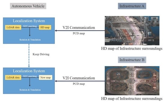
Real-time map data transmission requires communication equipment for transmission between infrastructure and vehicles. Initially, the infrastructure server in a specific area transmits map data to the vehicle using a roadside unit (RSU). In the vehicle, data are transmitted from the infrastructure using an access point (AP), such as an attached antenna. Typically, communication is achieved using a robot operating system (ROS) to exchange data in a 5 GHz band WiFi wireless network environment. When a 3D point cloud HD map around the infrastructure is transmitted, the vehicle performs localization using the transmitted map data. An overview of the communication system is shown in Figure 1.

LiDAR localization requires four components: hardware, such as sensors and vehicles, to acquire actual data to match; calibration steps, to acquire correct data for hardware; algorithms, to perform pose estimation; and, finally, an HD map to achieve localization. Accurate localization can only be performed when all four parts are operational. Figure 2 shows a flow diagram of an autonomous driving car with the LiDAR sensor attached, and the localization system used for the LiDAR localization experiment.

The autonomous vehicle used in the experiment was based on a minibus of a larger size. It was equipped with a 64-channel LiDAR sensor in the front, 16-channel LiDAR sensors on both sides at the bottom of the A pillars, and a 16-channel LiDAR on the upper part of the rear trunk for rear detection. The vehicle also had separate vision sensors, GPS, IMU, and other sensors for autonomous driving, but they were not utilized in this experiment. The coverage of the attached sensors is illustrated in Figure 3. The four LiDAR sensors mounted on the vehicle were connected to an Ethernet hub, which transmitted raw data to PCs. Various algorithms were then applied to perform localization as the final step.

The localization process involves downloading a 3D sub map from the infrastructure via V2I communication, and then performing matching using the NDT algorithm with the scan data from the autonomous vehicle. The map-matching algorithm utilizes the NDT algorithm. Detailed information about the algorithm can be found in this study [25]. The NDT algorithm calculates the vehicle’s displacement by comparing the normal distribution of the grid, which is uniformly divided between the registered map data and the scanned LiDAR point data. When representing the coordinates of ith points within the grid as ‘$x_i$’, the mean $\mu$ and covariance $\sum$ of the distribution can be expressed as follows.

$$\mu =\frac{1}{n}{\displaystyle \sum }_{i=1}^n{x}_i,$$

(1)

$$\sum =\frac{1}{n}{\displaystyle \sum }_{i=1}^n(x_i-\mu ){(x_i-\mu )}^T$$

(2)

The probability $p\left(x\right)$, modeled by the normal distribution N($\mu$,∑), which includes x, is as follows.

$$p\left(x\right)~e^{-\frac{{\left(x-\mu \right)}^T{\sum }^{-1}(x-\mu )}{2}}$$

(3)

In two dimensions, the coordinate transformation equation for spatial mapping T is given by

$$\begin{gathered} \mathbf{T}: \left(\begin{array}{c}{x}^{\prime }\\ y^{\prime }\end{array}\right)=\left(\begin{array}{cc}\mathrm{c}\mathrm{o}\mathrm{s}\varphi & -\mathrm{s}\mathrm{i}\mathrm{n}\varphi \\ \mathrm{s}\mathrm{i}\mathrm{n}\varphi & \mathrm{c}\mathrm{o}\mathrm{s}\varphi \end{array}\right)\left(\begin{array}{c}x\\ y\end{array}\right)+\left(\begin{array}{c}{t}_x\\ t_y\end{array}\right) \\ =\left(\begin{array}{c}x\mathrm{c}\mathrm{o}\mathrm{s}\varphi -y\mathrm{s}\mathrm{i}\mathrm{n}\varphi +t_x\\ x\mathrm{s}\mathrm{i}\mathrm{n}\varphi +y\mathrm{c}\mathrm{o}\mathrm{s}\varphi +t_y\end{array}\right) \end{gathered}$$

(4)

For two sequentially scanned data over time, $t_x$ and $t_y$ indicate the amount of translation, while $\varphi$ represents the amount of rotation. The mapping is conducted between the initial scan data and the following scan data, calculating the normal distribution and finding the optimal matching using the score of Equation (5). $\mathrm{P}$ represents the vector of parameters used for estimating. $x_i$ represents a sample of scanned LIDAR points, and $x_i^{\prime }$ represents the $x_i$ that has been sorted by the parameters in $\mathrm{P}$. The equation is expressed as $x_i^{\prime }=\mathbf{T}(x_i,\mathrm{P})$. The score of $\mathrm{P}$, which represents the optimal value of the matching, is defined as the following equation:

$$\mathrm{S}\mathrm{c}\mathrm{o}\mathrm{r}\mathrm{e}(\mathrm{P})={\displaystyle \sum }_{i=1}^n{e}^{-\frac{{\left(x_i^{\prime }-{\mu }_i\right)}^T{\sum }^{-1}\left(x_i^{\prime }-{\mu }_i\right)}{2}}$$

(5)

To optimize the mapping function, the process of finding the optimal parameters P that minimize the function $f$ is employed using the Newton algorithm. The parameters P that minimize the function are found using the gradient, $\mathit{g}$, of the function, $f$, and the Hessian matrix, H. $s$ is a summand of score.

$$\mathbf{H}∆\mathrm{p}=-\mathit{g}$$

(6)

$$g_i=\frac{𝜕f}{𝜕p_i}$$

(7)

$$H_{ij}=\frac{𝜕f}{𝜕p_i𝜕p_j}$$

(8)

$$\mu =x_i^{\prime }-{\mu }_i,\hspace{0.17em}s=-e^{\frac{-{\mu }^T{\sum }^{-1}\mu }{2}}$$

(9)

The partial derivative of $\mu$ with respect to $P_i$ can be represented by $x_i^{\prime }$, and the gradient of the score function can be calculated using Equation (9) as a summand. Therefore, the partial derivative of $\mu$ can be expressed as the Jacobian matrix $J_T$ of T. The gradient and Hessian are constructed using the partial derivatives of the score function with respect to all parameters.

$${\tilde{g}}_i=-\frac{𝜕s}{𝜕p_i}=-\frac{𝜕s𝜕\mu }{𝜕\mu 𝜕p_i}={\mu }^T{{\displaystyle \sum }}^{-1}\frac{𝜕\mu }{𝜕p_i}{e}^{\frac{-{\mu }^T{\sum }^{-1}\mu }{2}}$$

(10)

$$J_T=\left(\begin{array}{ccc}1& 0& -x\mathrm{s}\mathrm{i}\mathrm{n}\varphi -y\mathrm{c}\mathrm{o}\mathrm{s}\varphi \\ 1& 1& x\mathrm{c}\mathrm{o}\mathrm{s}\varphi -y\mathrm{s}\mathrm{i}\mathrm{n}\varphi \end{array}\right)$$

(11)

The Hessian matrix H can be expressed as shown below Equation (12), and the second partial derivative of $\mu$ can also be expressed using the equation below Equation (13).

$$\begin{gathered} {\tilde{H}}_{ij}=-\frac{𝜕s}{𝜕p_i𝜕p_j}=-e^{\frac{-{\mu }^T{{\displaystyle \sum }}^{-1}\mu }{2}}\left(\left(-{\mu }^T{{\displaystyle \sum }}^{-1}\frac{𝜕\mu }{𝜕p_i}\right)\left(-{\mu }^T{{\displaystyle \sum }}^{-1}\frac{𝜕\mu }{𝜕p_j}\right) \\ \hspace{1em}\hspace{1em}\hspace{1em}\hspace{1em}\hspace{1em}+\left(-{\mu }^T{{\displaystyle \sum }}^{-1}\frac{{𝜕}^2\mu }{𝜕p_i𝜕p_j}\right)+\left(-{\frac{𝜕{\mu }^T}{𝜕p_j}{\displaystyle \sum }}^{-1}\frac{𝜕\mu }{𝜕p_i}\right)\right) \end{gathered}$$

(12)

$$\frac{{𝜕}^2\mu }{𝜕p_i𝜕p_j}=\left\{\begin{array}{c}\left(\begin{array}{c}-x\mathrm{c}\mathrm{o}\mathrm{s}\varphi +y\mathrm{s}\mathrm{i}\mathrm{n}\varphi \\ -x\mathrm{s}\mathrm{i}\mathrm{n}\varphi -y\mathrm{c}\mathrm{o}\mathrm{s}\varphi \end{array}\right),\hspace{1em}\hspace{1em}\hspace{1em}i=j=3\\ \left(\begin{array}{c}0\\ 0\end{array}\right),\hspace{1em}\hspace{1em}\hspace{1em}otherwise\end{array}\right\}$$

(13)

The Hessian matrix is used to optimize the NDT function and perform position estimation. By computing the derivatives of the NDT function using the Hessian matrix, necessary updates and corrections for position estimation can be performed. The Hessian matrix provides information about the curvature and second-order derivatives of the NDT function, allowing for the efficient optimization and refinement of the estimated position.

In summary, sensors such as GPS, inertial measurement unit (IMU), vision, radar, and LiDAR are used for the localization of autonomous vehicles. The most common method for accurate location measurements is localization using GPS and LiDAR sensors. However, LiDAR localization requires a high-capacity HD map, which can burden the autonomous driving system. In one study, a method was employed to reduce the map size of an HD map and perform localization using GPS and IMU [26]. The existing 3D point cloud-based HD map has a large file size, so instead of reducing the file size, GPS and IMU were utilized to preserve the accuracy of localization. This approach aims to alleviate the computational power burden and ensure real-time performance for localization in autonomous vehicles. However, using this approach, autonomous driving is not possible in areas without a map. The proposed V2I system addresses these problems.

4. Methods

The autonomous vehicle used in this experiment was equipped with four LiDAR sensors. The sensors comprised a 64-channel LiDAR in the front, a 16-channel LiDAR located above both front fenders, and a 16-channel LiDAR attached to the rear of the vehicle. The sensors were calibrated considering the pose for each sensor attachment location to facilitate the acquisition of sensor data. Smooth communication up to a line of sight of 500 m was confirmed.

Both the infrastructure RSU and vehicle AP equipment used the RT-AC68U model equipped with three external antennas with a 12 dBi output, and a IEEE 802.11ac standard WiFi 5 network [27]. The bandwidths used were 5 GHz band 80 MHz, with the Tx Power set to 1000 mW.

The PCs used in the experiment were set to ROS Melodic in the Ubuntu 18.04 LTS environment. ROS communication is a communication method provided by ROS, in which many components exchange topics using nodes under one master management module. The detailed specifications of the sensors and equipment used in the experiment are summarized in

Table 1. Experimental environment.

	Manufacturer	Model	Qty	Specification	Remarks
Sensor	Velodyne	VLP 16	3	16 ch. Vertical FOV 30 deg. Vertical resol. 2 deg. Horizontal resol. 0.1–0.4 deg.	Left/Right/Rear
	Ouster	OS1 64	1	64 ch. Vertical FOV 45 deg. Vertical resol. 0.7 deg. Horizontal resol. 0.35 deg	Front
AP/RSU	ASUS	RT-AC68U	2	Antenna output 12 dBi IEEE 802.11ac, WiFi5 5 GHz band 80 MHz bandwidth Tx power 1000 mW	Infra./vehicle
PC	LENOVO	Thinkpad/ Legion 5 pro	2	Ubuntu 18.04 LTS ROS Melodic	Infra./vehicle
Vehicle	Hyundai	Solati	1	Mini bus
	Kia	Sportage	1	Mid-size SUV

. If infrastructure PCs and vehicle PCs are connected to the same ROS Master address, anyone can subscribe to the ROS Topic that the infrastructure publishes. Thus, even if multiple vehicles are connected, each can receive an HD map without obstructions. Not only can it establish 1:1 communication links, but it also enables 1:N communication, allowing a single infrastructure to transmit surrounding map data to multiple vehicles.

Depending on the number of connected vehicles, the speed may decrease due to the bandwidth limitations. This can be mitigated by calculating the traffic flow of vehicles and employing techniques such as bandwidth allocation and partitioning.

The NDT-matching algorithm was used as the LiDAR localization algorithm in the experiment. The NDT-matching algorithm was used for localization with the prebuilt HD map, because the point cloud registration method is more efficient than the scan-matching method.

Map-matching was conducted on a proving ground (PG) with a length of 1 km and width of 400 m; the capacity of the entire PG point cloud map reached 4.64 GB. Therefore, the entire map was divided into sections of approximately 200 m in width and 300 MB in capacity, and experiments were conducted using maps of different sizes that were voxelized and lightened. The optimal environment was determined by measuring the capacity and matching accuracy based on the density of the map, the communication delay based on the infrastructure and vehicle distance, and the communication delay based on the speed of the vehicle. Figure 4 shows the sub map that was segmented from the HD map of the entire PG and the map surrounding the infrastructure, while Figure 5 is the original image of the segmented sub map data zoomed in. Figure 6 and Figure 7 show the results of applying voxelization filters of different sizes to the sub map.

5. Experiments and Results

The experiment was conducted in two steps. In the first step, we measured the time taken to match by loading the map of the autonomous vehicle without communication in an environment in which the same hardware is set. The loading time required to calculate the initial position by loading each map was measured for different map sizes based on the voxelization filter size. The loading time represents the average of 20 repetitions for each map. By comparing the loading time of the matching system and the matching score of each map, we evaluated the reliability of the HD map with usable accuracy.

Table 2. A comparison table of map loading time without V2I, based on map size.

Source	Map Size	Voxelization Filter Size (m)	Loading Time (s)	Remarks
Map A	4.64 GB	N	40.41	Full map
	304 MB	N	1.98	Sub map
	41.2 MB	0.1	1.4	Voxelized submap
	3.1 MB	0.5	1.37	Voxelized submap
	931.8 KB	1	1.35	Voxelized submap
	287 KB	2	1.34	Voxelized submap

shows the loading times for the HD map of the entire PG, sub maps, and downsampled sub maps of different sizes, until the localization system starts matching them, without communication with the vehicle’s PC, which has the maps. The loading times vary depending on the size of the maps. According to the experimental results, it took 40 s to load the original PG HD map and start localization, while for the sub maps, it only took 1.98 s, which is about 1/20th of the original time. Although the loading time decreased as the voxelization filter size decreased, it generally saturated at around 1.4 s. Based on these results, to achieve fast transmission and high map-matching performance, experiments were conducted using sub maps voxelized at a size of 0.1 m.

In the second step, we measured the map data transmission time for each capacity according to the degree of weight reduction at various distances. We experimentally determined the maximum reliable infrastructure distance when using V2I by measuring the change in communication delay time with increasing distance from the infrastructure. In addition, we determined the optimal HD map condition.

The following results are obtained by measuring the time taken to receive the map from the infrastructure according to the distance for each map set, fully upload it, and start matching. Similarly, the above experiment was tested ten times for each category, the average of which is shown in the table. Maps A, B, and C are three sub maps of the PG shown in Figure 4. They were divided into partitions of equal size for experimentation purposes, ensuring that neighboring regions were mapped at the same capacity. The experimental results show that the change in delay with increasing distance is limited to 2–3 s, with no significant difference within 100 m.

In

Table 3. Map data transmission time comparison table according to distance.

Source	Map Size	Initial Loading Time (s)—Range			Computation Time (ms)
		0 m	50 m	100 m
Map A	304 MB	27.92	32.8	30.02	144.4
	41.2 MB	3.17	4.1	4.4	42.1
	3.1 MB	2.04	2.53	2.7	8.2
	931.8 KB	1.91	1.77	1.51	-
	287 KB	2.2	1.91	1.85	-
Map B	304 MB	27.45	32.17	29.02	148.5
	41.2 MB	4.47	5.51	4.27	44.1
	3.1 MB	1.72	1.87	2.24	8.9
	931.8 KB	1.72	2.1	2.16	-
	287 KB	1.85	1.71	1.91	-
Map C	304 MB	28.63	28.11	29.27	146.4
	41.2 MB	4.47	3.81	5.04	48.4
	3.1 MB	1.72	1.99	2.89	8.7
	931.8 KB	1.72	2.11	2.11	-
	287 KB	1.85	1.98	2.04	-

, the initial loading time values represent the average time it takes for the map to be transmitted to the vehicle’s localization system via V2I, and for the initial pose to be established. Computation time indicates the average processing speed of the localization system for each sequence after the initial pose calculation. Once the map is downloaded from the infrastructure and the initial pose is computed, the localization system operates at a constant speed similar to that of an onboard system. The time required to process a single sequence of data for map-matching was measured in milliseconds (ms). Sub maps with voxelization filter sizes larger than 1 resulted in sparse maps, making it difficult to achieve accurate localization. As a result, the localization process was not successful under these circumstances.

Furthermore, in terms of the experimental conditions, once the communication between the vehicle and the infrastructure was established, the difference in vehicle speed did not affect the time required to download the map. Therefore, the experiments were conducted at a constant speed of 50 km/h.

In summary, the benefits of voxelized separation maps generated using infrastructure were confirmed; these maps can achieve a reduction of 99% (4.64 GB, 41.2 MB) in capacity and approximately 35 s (40.41 s, 4.4 s) in time for HD maps within 100 m of infrastructural RSUs, compared to the conventional LiDAR localization method. Furthermore, the computation time exhibited an average delay of around 40 ms and achieved a performance of over 20 Hz, satisfying real-time requirements.

Figure 8 depicts the real-time map-matching process of an autonomous vehicle passing through an area with infrastructure 1 and infrastructure 2, receiving different sub maps from each. In (a), the vehicle performs localization using the map received from infrastructure 1, and reaches the end of the map. In (b), the vehicle downloads a new sub map from infrastructure 2, and performs localization immediately. To create a more extreme environment, the overlapping sections of the sub maps were set to be short, i.e., within 20 m, in this experiment.

Figure 9 depicts the coordinates obtained during the localization process of an autonomous vehicle driving through three neighboring sub maps received via V2I, as well as the coordinates measured by the localization system utilizing the HD map of the entire driving environment. When applying the method proposed in this study, there was little difference between autonomous vehicles equipped with the complete HD map of the driving environment for positioning and those utilizing the sub map-matching approach.

The root mean square errors (RMSE) calculated for the estimated coordinate differences between HD map-matching and sub map-matching for the three segments were 0.004, 0.167, and 0.047, respectively, while the overall RMSE for the entire driving route was 0.111. These results indicate that the system’s accuracy demonstrates an acceptable level of error for practical autonomous driving scenarios. Furthermore, the use of small-sized maps for localization offers significant advantages in terms of capacity limitations, as there is no need to possess the entire map; small-sized maps also provide computational benefits.

6. Conclusions

This study proposes a LiDAR localization method using V2I to address the issue of the large-capacity HD maps required for conventional localization methods. Using V2I, HD maps within a 200 m radius of each infrastructural RSU are transmitted to the vehicle, which downloads them and performs real-time localization. The capacities of the separated maps are approximately 6.5% of the total map capacity; the lightweight voxelized map is approximately 40 MB, 99% smaller than the total map. In this study, real-time map-matching was achieved in a vehicle running a lightweight map after receiving transmission from the infrastructure. In addition, reliable operation was confirmed for various speed and distance conditions.

The proposed system can potentially overcome the biggest obstacles in existing methods, such as limited data storage space, huge computational load (owing to large map size), and unavailability of maps to achieve real-time performance. In addition, considering the ease of infrastructure construction and the possibility of networking all vehicles with proper communication, it is considerably more economical than the existing methods.

The reason for proposing a positioning system based solely on LiDAR sensors in this study is to ensure redundancy in the localization system of autonomous vehicles. It is understood that using additional systems such as GNSS and IMU would naturally yield more accurate results. However, when the vehicle enters an area in which satellite signals are not available, the proposed approach suggests utilizing infrastructure-based map-matching using precise maps as an alternative for localization.

Such research can be utilized in future applications such as an auto valet parking system, in which unmanned electric vehicles without human occupants need to approach the nearest building’s parking lot for charging during autonomous driving. In such cases, the vehicle may receive precise map data of the building through communication, and follow the instructions of the infrastructure control system to park in the designated area for charging.

Even if the autonomous vehicle does not have the map, by using the infrastructure communication system to transmit the detailed map of the underground parking lot of a building to the approaching vehicle, it may easily navigate to the specified parking slot using accurate position information. This may help prevent accidents during parking, and save time that would otherwise be spent searching for parking spaces.

References

- Pendleton, S.D.; Andersen, H.; Du, X.; Shen, X.; Meghjani, M.; Eng, Y.H.; Rus, D.; Ang, M.H. Perception, Planning, Control, and Coordination for Autonomous Vehicles. Machines 2017, 5, 6. [Google Scholar] [CrossRef] [Green Version]
- Laconte, J.; Kasmi, A.; Aufrère, R.; Vaidis, M.; Chapuis, R. A Survey of Localization Methods for Autonomous Vehicles in Highway Scenarios. Sensors 2022, 22, 247. [Google Scholar] [CrossRef] [PubMed]
- Zhang, Y.; Wang, L.; Wang, J. Real-time localization method for autonomous vehicle using 3DLIDAR. Dyn. Veh. Roads Tracks 2017, 1, 271–276. [Google Scholar]
- Chen, D.; Weng, J.; Huang, F.; Zhou, J.; Mao, Y.; Liu, X. Heuristic Monte Carlo Algorithm for Unmanned Ground Vehicles Realtime Localization and Mapping. IEEE Trans. Veh. Technol. 2020, 69, 10642–10655. [Google Scholar] [CrossRef]
- Jo, K.; Keonyup, C.; Myoungho, S. GPS-bias correction for precise localization of autonomous vehicles. In Proceedings of the 2013 IEEE Intelligent Vehicles Symposium (IV), Gold Coast, QLD, Australia, 23–26 June 2013; pp. 636–641. [Google Scholar]
- Yi, S.; Worrall, S.; Nebot, E. Integrating Vision, Lidar and GPS Localization in a Behavior Tree Framework for Urban Autonomous Driving. In Proceedings of the IEEE International Intelligent Transport Systems Conference, Indianapolis, IN, USA, 19–22 September 2021; pp. 3774–3780. [Google Scholar]
- Xia, X.; Meng, Z.; Han, X.; Li, H.; Tsukiji, T.; Xu, R.; Ma, J. An automated driving systems data acquisition and analytics platform. Transp. Res. Part C Emerg. Technol. 2023, 151, 104120. [Google Scholar] [CrossRef]
- Park, Y.; Park, H.; Woo, Y.; Choi, I.; Han, S. Traffic Landmark Matching Framework for HD-Map Update: Dataset Training Case Study. Electronics 2022, 11, 863. [Google Scholar] [CrossRef]
- Janai, J.; Guney, F.; Behl, A.; Geiger, A. Computer vision for autonomous vehicles: Problems, datasets and state of the art. In Foundations and Trends® in Computer Graphics and Vision; Now Publishers: Boston, MA, USA, 2020; pp. 1–308. [Google Scholar]
- Oliver, P. Visual map matching and localization using a global feature map. In Proceedings of the 2008 IEEE Computer Society Conference on Computer Vision and Pattern Recognition Workshops, Anchorage, AK, USA, 23–28 June 2008; pp. 1–7. [Google Scholar]
- Wided, S.M.; Mohamed, A.S.; Rabah, A. YOLOv5 Based Visual Localization For Autonomous Vehicles. In Proceedings of the 29th European Signal Processing Conference (EUSIPCO), Dublin, Ireland, 23–27 August 2021; pp. 746–750. [Google Scholar]
- Campbell, S.; O’Mahony, N.; Krpalcova, L.; Riordan, D.; Walsh, J.; Murphy, A.; Ryan, C. Sensor technology in autonomous vehicles: A review. In Proceedings of the 29th Irish Signals and Systems Conference (ISSC), Belfast, UK, 21–22 June 2018; pp. 1–4. [Google Scholar]
- Erik, W.; John, F. Vehicle localization with low cost radar sensors. In Proceedings of the 2016 IEEE Intelligent Vehicles Symposium (IV), Gotenburg, Sweden, 19–22 June 2016; pp. 864–870. [Google Scholar]
- Bilik, I.; Longman, O.; Villeval, S.; Tabrikian, J. The rise of radar for autonomous vehicles: Signal processing solutions and future research directions. IEEE Signal Process. Mag. 2019, 36, 20–31. [Google Scholar] [CrossRef]
- Kwon, S.; Yang, K.; Park, S. An effective kalman filter localization method for mobile robots. In Proceedings of the 2006 IEEE/RSJ International Conference on Intelligent Robots and Systems, Beijing, China, 9–15 October 2006; pp. 1524–1529. [Google Scholar]
- Mendes, E.; Koch, P.; Lacroix, S. ICP-based pose-graph SLAM. In Proceedings of the 2016 IEEE International Symposium on Safety, Security, and Rescue Robotics, New York, NY, USA, 26–31 August 2016; pp. 195–200. [Google Scholar]
- Liu, J.; Sun, Q.; Fan, Z.; Jia, Y. TOF lidar development in autonomous vehicle. In Proceedings of the 2018 IEEE 3rd Optoelectronics Global Conference, Shenzhen, China, 4–7 September 2018; pp. 185–190. [Google Scholar]
- Zhang, J.; Singh, S. LOAM: Lidar odometry and mapping in real-time. Robot. Sci. Syst. 2014, 2, 1–9. [Google Scholar]
- Takubo, T.; Kaminade, T.; Mae, Y.; Ohara, K.; Arai, T. NDT scan matching method for high resolution grid map. In Proceedings of the 2009 IEEE/RSJ International Conference on Intelligent Robots and Systems, St. Louis, MO, USA, 11–15 October 2009; pp. 1517–1522. [Google Scholar]
- Shoubin, C.; Hao, M.; Changhui, J.; Baoding, Z.; Weixing, X.; Zhenzhong, X.; Qingquan, L. NDT-LOAM: A Real-Time Lidar Odometry and Mapping With Weighted NDT and LFA. IEEE Sens. J. 2022, 22, 3660–3671. [Google Scholar]
- Chiang, K.; Srinara, S.; Tsai, S.; Lin, C.; Tsai, M. High-Definition-Map-Based LiDAR Localization Through Dynamic Time-Synchronized Normal Distribution Transform Scan Matching. IEEE Trans. Veh. Technol. 2023, 99, 1–13. [Google Scholar] [CrossRef]
- Shin, D.; Park, K.-m.; Park, M. High Definition Map-Based Localization Using ADAS Environment Sensors for Application to Automated Driving Vehicles. Appl. Sci. 2020, 10, 4924. [Google Scholar] [CrossRef]
- Tsushima, F.; Kishimoto, N.; Okada, Y.; Che, W. Creation of high definition map for autonomous driving. Int. Arch. Photogramm. Remote Sens. Spat. Inf. Sci. 2020, 43, 415–420. [Google Scholar] [CrossRef]
- Milanés, V.; Villagrá, J.; Godoy, J.; Simó, J.; Pérez, J.; Onieva, E. An intelligent V2I-based traffic management system. IEEE Trans. Intell. Transp. Syst. 2012, 13, 49–58. [Google Scholar] [CrossRef] [Green Version]
- Biber, P.; Straßer, W. The normal distributions transform: A new approach to laser scan matching. In Proceedings of the 2003 IEEE/RSJ International Conference on Intelligent Robots and Systems, Las Vegas, NV, USA, 27–31 October 2003; Volume 3, pp. 2743–2748. [Google Scholar]
- Ma, W.; Tartavull, I.; Bârsan, I.; Wang, S.; Bai, M.; Mattyus, G.; Urtasun, R. Exploiting sparse semantic HD maps for self-driving vehicle localization. In Proceedings of the 2019 IEEE/RSJ International Conference on Intelligent Robots and Systems (IROS), Macau, China, 3–8 November 2019; pp. 5304–5311. [Google Scholar]
- Available online: https://www.electronics-notes.com/articles/connectivity/wifi-ieee-802-11/802-11ac.php (accessed on 8 May 2023).