Underwater Noise Modeling and Its Application in Noise Classification with Small-Sized Samples

Abstract

Underwater noise classification is of great significance for identifying ships as well as other vehicles. Moreover, it is helpful in ensuring a marine habitat-friendly, noise-free ocean environment. But a challenge we are facing is the small-sized underwater noise samples. Because noise is influenced by multiple sources, it is often difficult to determine and label which source or which two sources are dominant. At present, research to solve the problem is focused on noise image processing or advanced computer technology without starting with the noise generation mechanism and modeling. Here, a typical underwater noise generation model (UNGM) is established to augment noise samples. It is established by generating noise with certain kurtosis according to the spectral and statistical characteristics of the actual noise and filter design. In addition, an underwater noise classification model is developed based on UNGM and convolutional neural networks (CNN). Then the UNGM-CNN-based model is used to classify nine types of typical underwater noise, with either the 1/3 octave noise spectrum level (NSL) or power spectral density (PSD) as the input features. The results show that it is effective in improving classification accuracy. Specifically, it increases the classification accuracy by 1.59%, from 98.27% to 99.86%, and by 2.44%, from 97.45% to 99.89%, when the NSL and PSD are used as the input features, respectively. Additionally, the UNGM-CNN-based method appreciably improves macro-precision and macro-recall by approximately 0.87% and 0.83%, respectively, compared to the CNN-based method. These results demonstrate the effectiveness of the UNGM established in noise classification with small-sized samples.

1. Introduction

Underwater noise study is an important direction in underwater acoustics. The classification of underwater noise is of great significance for marine biological protection, ship identification, target positioning, and so on. In the era of big data, using machine learning methods to classify underwater noise has become a new trend. Unlike active experimental data collection, such as target localization, passive underwater noise (UN)collection is affected by cross-contamination between different noise sources. In many cases, it is difficult to determine and label which noise source or which two noise sources dominate. In other words, the current research status is characterized by a small number of samples in a large amount of data. However, most machine learning techniques require neural networks (NN) models trained on a large amount of data. This condition restricts the application of deep learning techniques in UN classification. Extracting and learning the features of UN from limited data resources is a major issue in UN classification that must be addressed. Four types of methods are currently available as solutions to small-sized sample learning. They are data augmentation (DA), transfer learning, metric learning, and meta-learning methods [1,2,3]. The DA-based approaches are subdivided into unlabeled data-based, data generation-based, and feature augmentation-based approaches. The advantage of this method is that it does not require adjustments to the model; it only needs to use auxiliary data or information to expand the data or enhance the features. The disadvantage is that it may introduce many noisy data or features, which may have a negative impact on classification performance [4,5,6]. Transfer learning methods mainly pre-train a model on source-domain samples similar to target-domain samples and subsequently transfer and apply the pre-trained model to the target scenario. These methods have highly limited applications due to their requirement for a large amount of labeled data in the source domain. In addition, they are not sufficiently flexible in terms of application scenarios and may lead to negative transfer [7,8]. Metric learning methods aim to ensure that cases of the same type are close to each other in the embedded space and that cases of different types are far away from each other. These methods classify unlabeled new cases based on their proximity to the labeled data in a given pre-trained deep-embedded space. This method is easy to calculate, but the accuracy of measuring similarity through distance will be reduced in the case of small-sized samples [9,10,11]. Meta-learning methods primarily train an NN model with generalization capabilities that are capable of learning abstract meta-features from relevant tasks. It has learning ability and can learn some knowledge beyond the training process, but its complexity is high and needs further improvement and development [12,13,14]. The available methods classify a small number of samples primarily based on new network techniques, new feature extraction, or transformation. No work carried out so far has considered underwater noise generation mechanisms.

On this basis, a UN generation model (UNGM) is established and used to classify UN with small-sized samples. In this model, UNGM is first proposed to simulate the typical UN. Then the simulated data are combined with measured data to form a combined dataset. Finally, convolutional neural networks (CNN) combined with UNGM is trained using the actual and combined dataset to produce accurate and robust classification results. In this method, the process of UNGM follows the noise generation mechanism, which can increase the measured data, so that it can solve the research gap faced in UN classification. To verify the method, nine classes of UN, including air-gun noise, mixed air-gun and vessel noise, ambient noise, and six vessels, are acquired. And they are simulated one time, two times, and six times to form the mixed data. For each dataset, they are randomly grouped into five mutually disjoint subsets of the same size. Four of the five subsets are used to train the classification model, while the remaining subset is used to test the classification model. And the process is repeated for all five possible combinations to get an accurate result.

Briefly, the main contributions of this study are as follows:

(1)

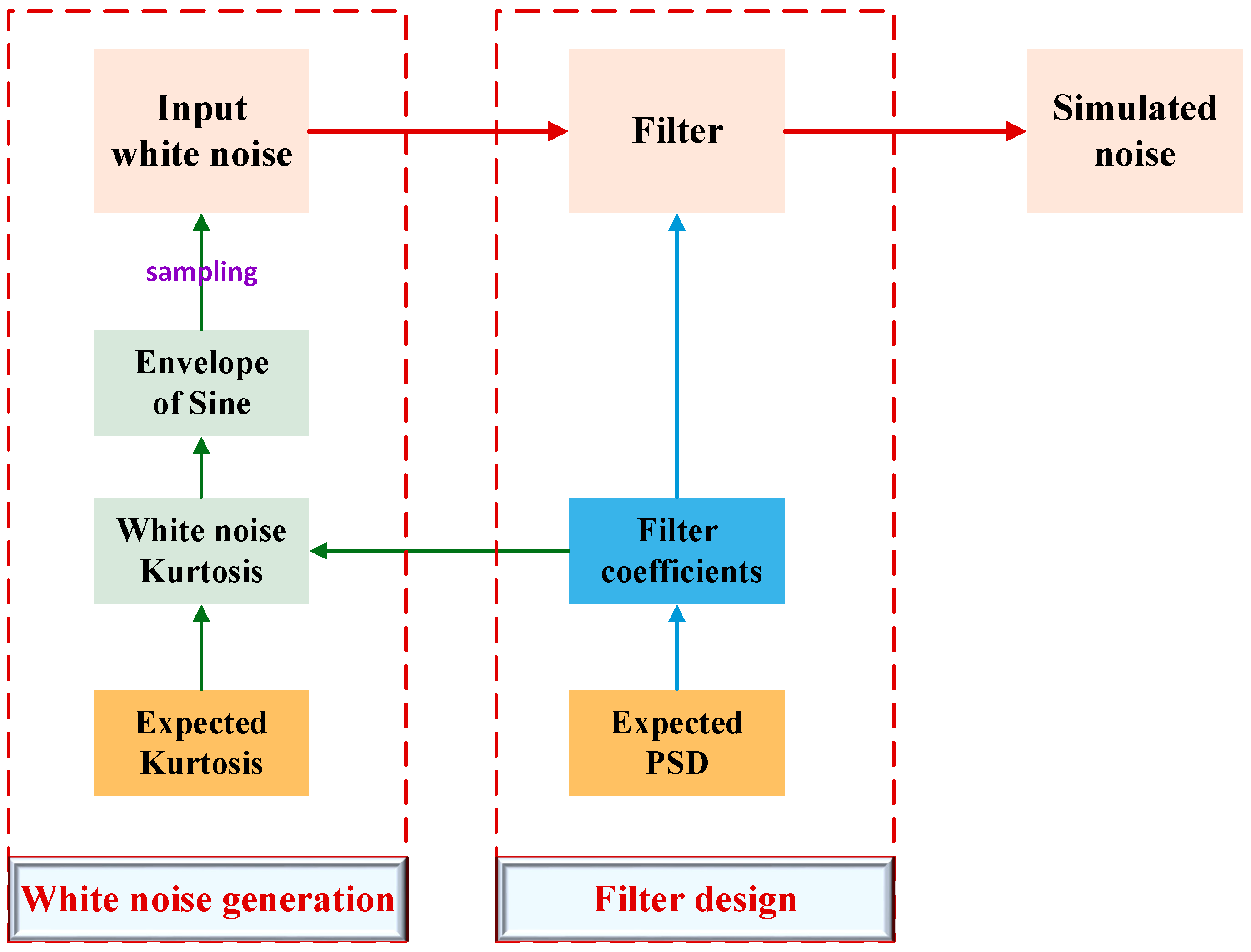
A UN generation model to simulate the nine typical noise types with certain PSD and kurtosis, which can augment the noise sample;

(2)

UN-generation model-based CNN that can classify nine sources of ocean noise, namely, air-gun noise, mixed air-gun and vessel noise, ambient noise, KeDiao vessel, and five fishing vessels;

(3)

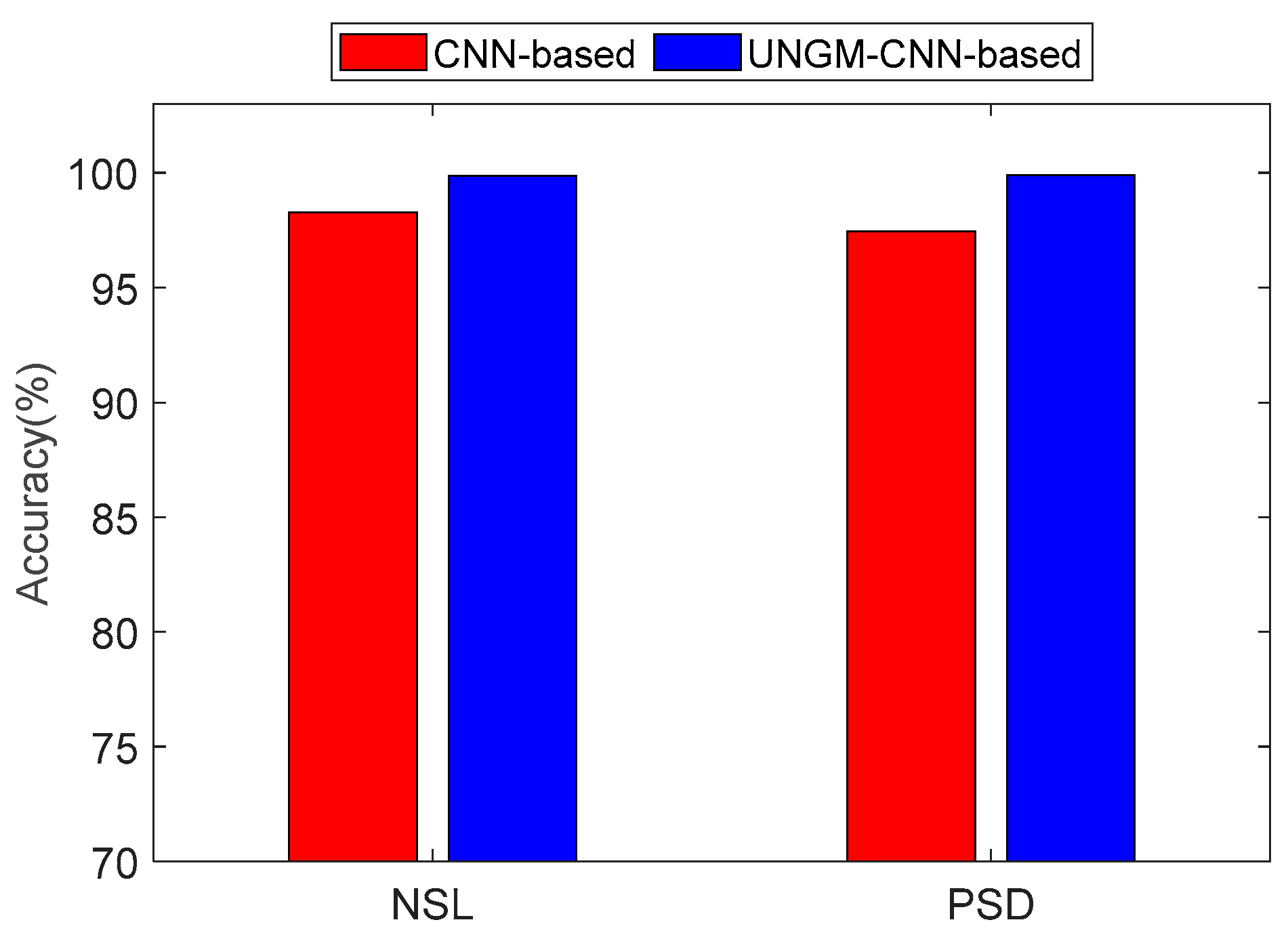
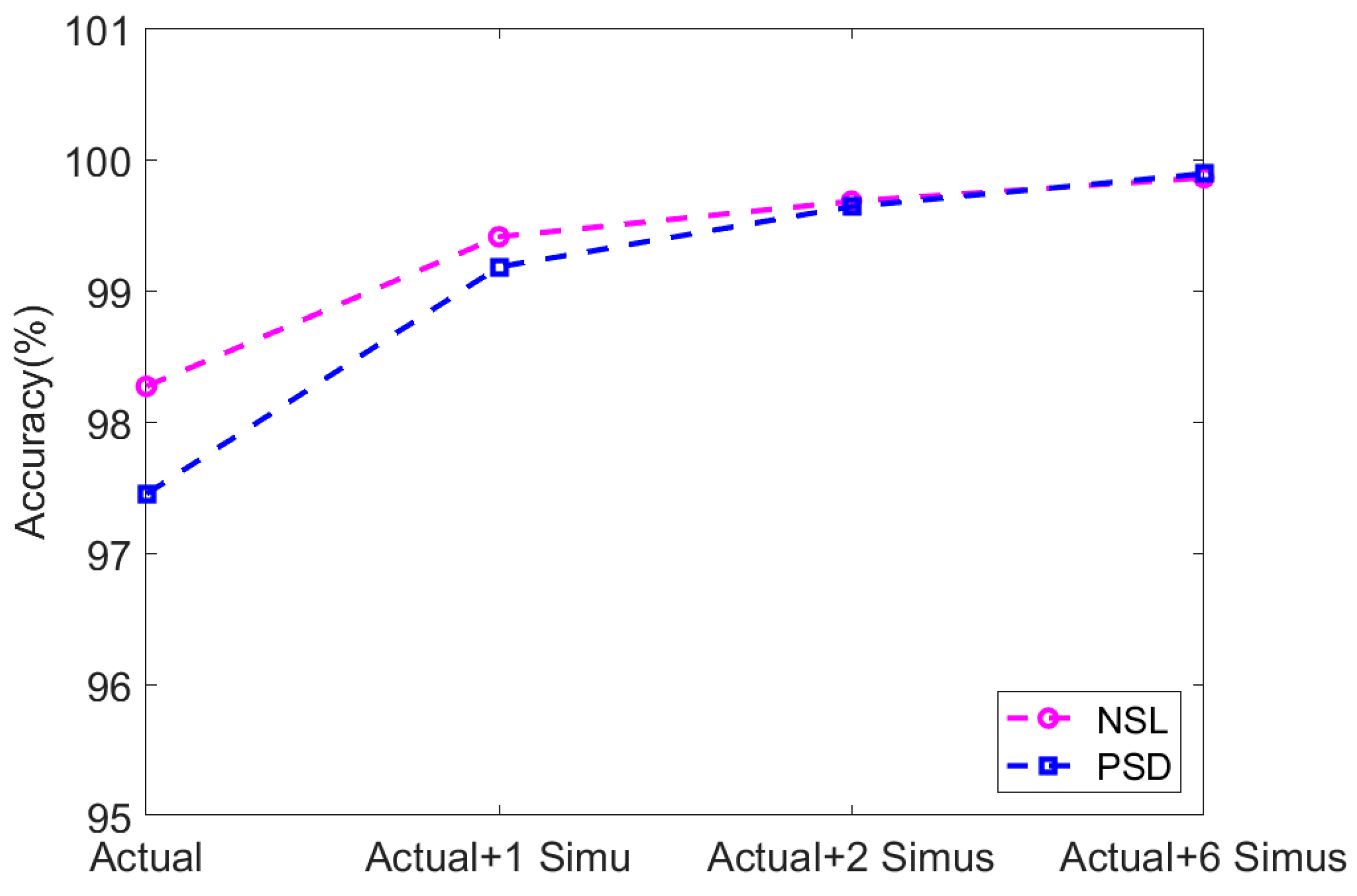
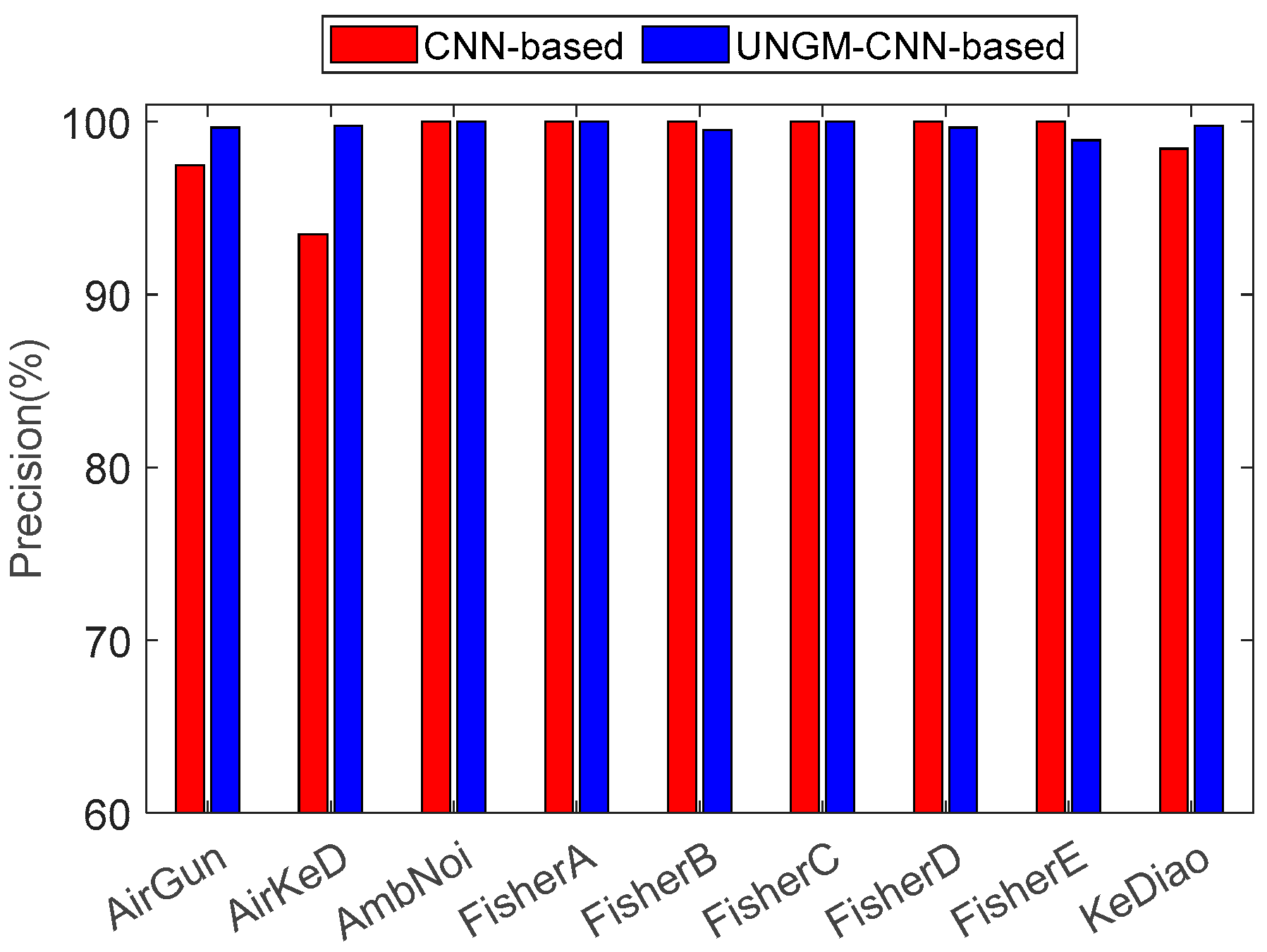
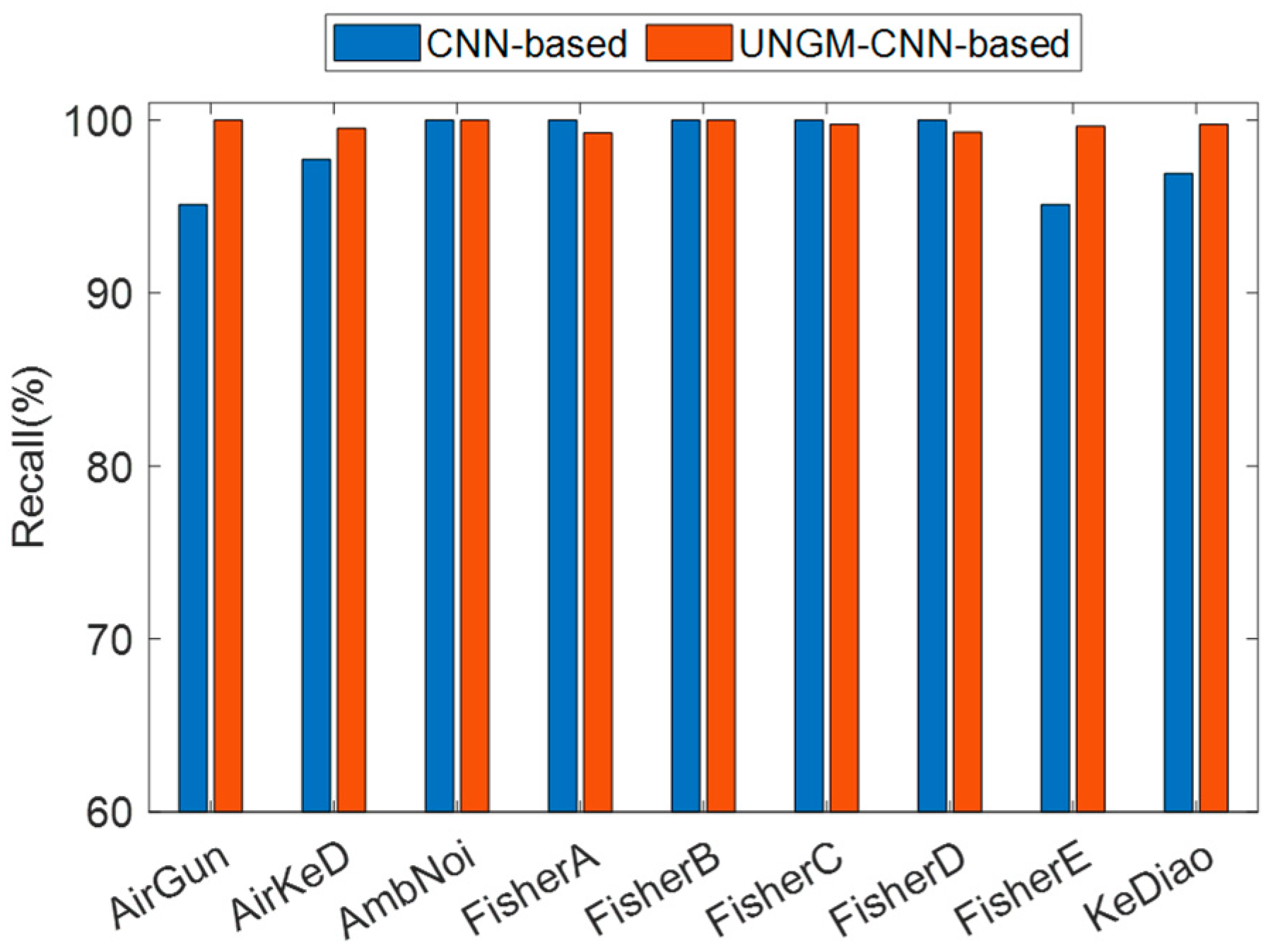
classification performance enhancement by combing a generation model and a CNN-based classification model. While augmenting the measured data with simulated data six times as large, it increases the classification accuracy by 1.59% and 2.44% when the NSL and PSD are used as the input features, respectively.

The remaining sections of the paper are organized as follows: In Section 2, the previous related work on UN classification is reviewed. Section 3 provides the methodology, which includes a generative model for UN and UNGM-CNN-based underwater noise classification. The experimental setup and analysis covering data collection, as well as the discussions, are detailed in Section 4. Finally, the conclusion is presented in Section 5.

2. Related Work

In recent years, cross-disciplinary research involving underwater acoustics and machine learning has garnered intense attention from researchers worldwide. New techniques integrated with machine learning (ML) or deepNNhave produced consequential research findings in several areas (e.g., underwater target recognition [15], sound source or target ranging and positioning [16,17], marine animal sound classification, seafloor sediment classification [18], underwater noise classification [19], and relationships between deep learning-based object detection technologies and geospatial big data management algorithms [20,21,22]) and have been developed for the identification of physical correlations or to provide interpretability.

2.1. Underwater Acoustics Related

Li et al. [23] proposed a deep-learning underwater object recognition method suitable for multichannel hydrophone arrays and subsequently used it to identify five types of targets through cascading of sub-channel features based on multichannel information. Wang et al. [24] introduced a deep transfer learning method for data containing target signal and UNmeasurements to facilitate underwater sound source ranging and subsequently validated its effectiveness at improving the ranging accuracy based on experimental data. Escobar-Amado et al. [25] detected and positioned seal vocalizations using convolutional neural networks (CNN). Zhong et al. [26] employed a CNN model to classify beluga detections, achieving an accuracy of 96.57%. Li et al. [27] developed a U-Net model based on a random mode-coupling matrix to recover distorted acoustic interference striations. Ekpez proposed a method for natural disasters classification, and the CNN model obtained a classification accuracy of 99.96%, whereas the LSTM obtained an accuracy of 99.90% [28]. Merchant ship-radiated noise was employed for seabed classification using an ensemble of deep learning (DL) algorithms by Escobar-Amado. The accuracy of the five networks was above 97% [29]. A siamese neural network (SNN) was used to detect, classify, and count the calls of four acoustic populations of blue whales, and it outperformed a CNN with a 2% accuracy improvement in population classification [30].

2.2. Underwater Noise Classification

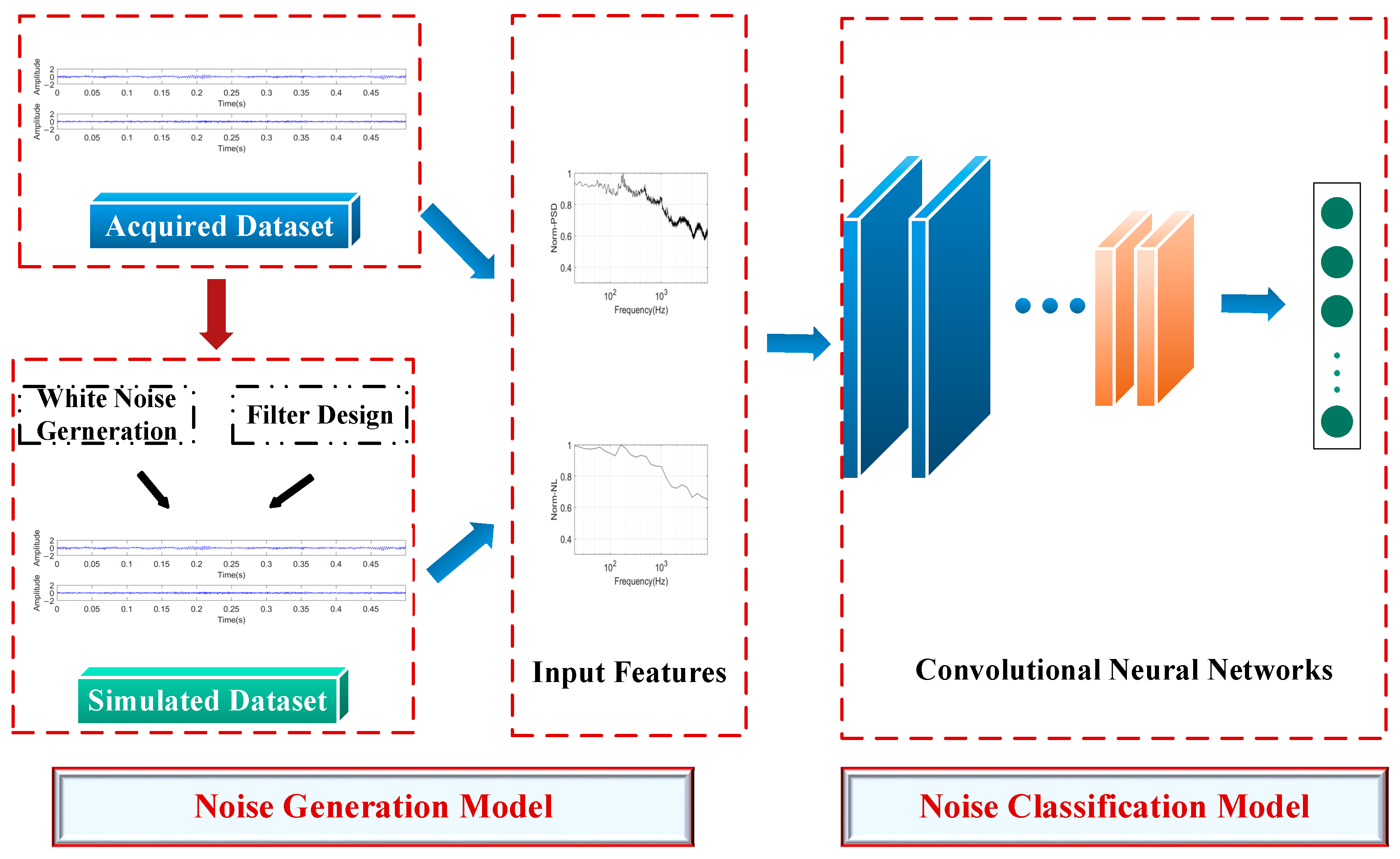
In terms of UN research, machine learning techniques have yielded some progressive results. Wu et al. [31] classified a total of 1049 ship-radiated noise samples using a fuzzy NN in conjunction with a statistical pattern recognition technique. The small number of samples used in this study, however, limited the classification’s performance and reliability. Wu and Yang [32] used a support vector machine (SVM) method to classify ship images based on their histograms of oriented gradients (HOG) and achieved an identification accuracy of 84.14%. Yang and Zhou [33] proposed an improved bi-coherence spectrum combined with a cyclic modulation spectrum and cross-correlation. Its subsequent use as a characteristic quantity for deep learning to classify five types of ship-radiated noise and towing sound sources produced a classification accuracy above 80%. Premus et al. [34] classified the underwater noise for rapid identification of surface vessel opening and closing behavior by using machine learning methods. Song et al. [35] classified five types of typical UN using a CNN and explained the classification results based on statistical analysis. Mishachandar [36] presented a CNN-based ocean noise classification and recognition system capable of classifying the vocalizations of cetaceans, fish, marine invertebrates, anthropogenic sounds, natural sounds, and unidentified ocean sounds from passive acoustic ocean noise recordings with 96.1% accuracy. The comparison of these studies is shown in

Table 1. Comparison of some studies of UN classification.

Reference	Method	Noise Type	Sample Size	Accuracy
[31]	Fuzzy neural network (FNN)	41 ships	1049	92.9%
[32]	Support vector machine (SVM)	5 ships	983	84.14%
[33]	SVM, random forest (RF), deep belief network (DBN)	4 ships + 1 drag source	30,000	91.2%
[34]	CNN	4 ships (trained on three vessels and applied to a fourth, to determine whether the vessel was opening or closing)	--	89.6%
[35]	CNN	5 ships	7225	98.95% (SNR = −10 dB)
[36]	CNN	Cetaceans, fishes, marine invertebrates, anthropogenic sounds, natural sounds, and the unidentified ocean sounds	560, then augment to 205,618	96.01%

.

It can be seen that most methods [31,32,33,34,35] only rely on measured data and try to improve classification performance by changing machine learning techniques. Reference [36] augmented the measured data by using traditional audio signal enhancement methods, including time shifting, pitch and speed shifting, and noise injection. The biggest advantage of this method is that it is simple and easy to operate, even without any underwater acoustic background. However, combining the physical principles of underwater acoustics with machine learning is what marine acoustics pursues. This is also what this study attempts to do, that is, to establish a noise generative model based on the noise generation mechanism to solve the small sample problem encountered in classification.

3. Methodology

The study consists of two parts: one is a noise generation model, and the other is a noise classification model. Figure 1 shows the specific framework of the proposed method.

In the first part, the model is achieved by generating white noise and designing a filter. It is used to simulate noise by 1 time, 2 times, and 6 times the acquired noise to form the simulated dataset. In the second part, a UNGM-CNN-based classification model is proposed. It is mainly composed of an input layer, convolution layers, pooling layers, fully connected layers, and an output layer. It is used to learn the difference between the features of different types of UN with a small number of measured samples and model-generated samples.

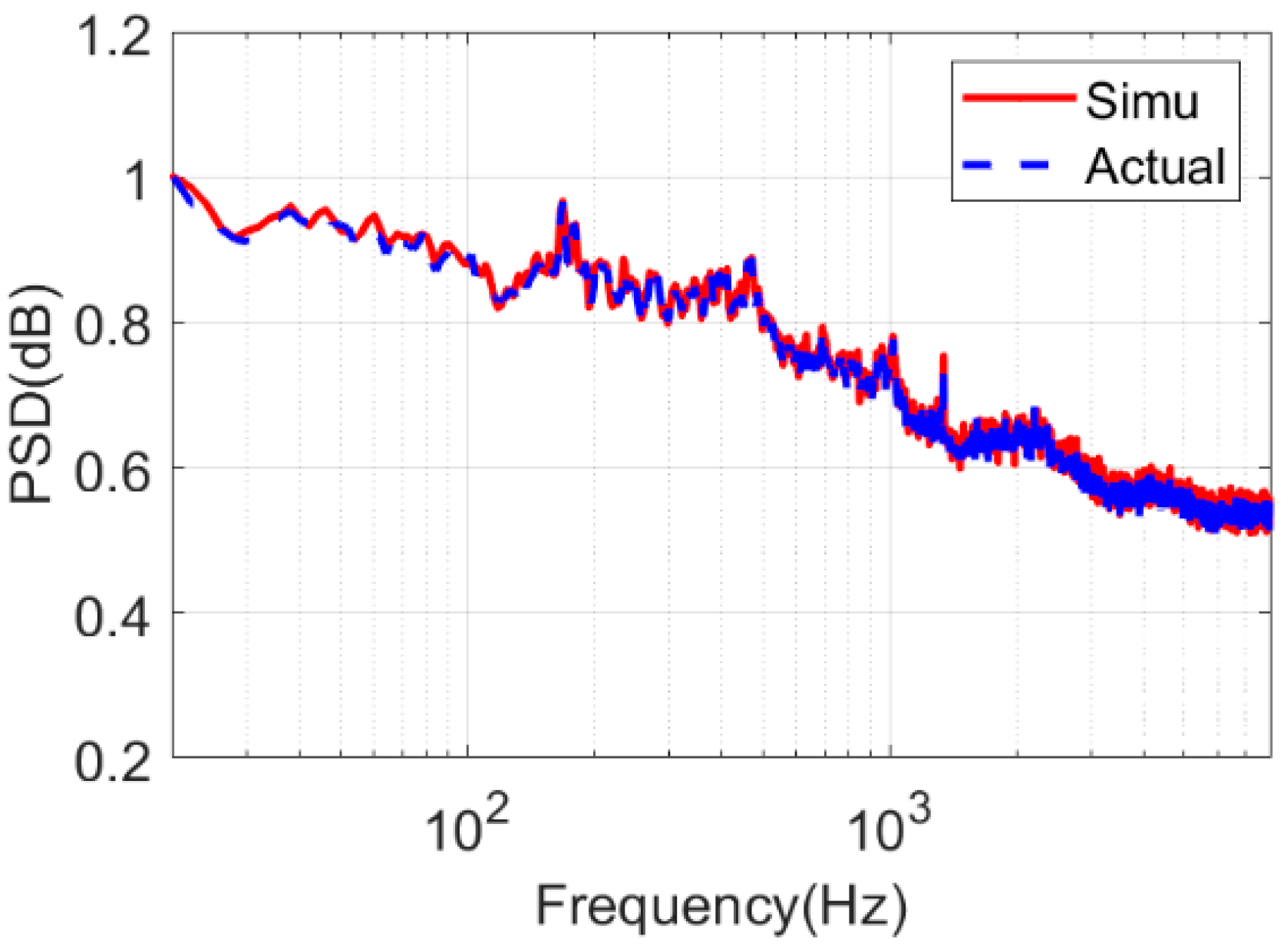
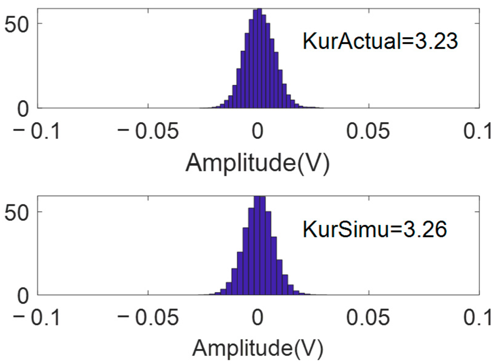
3.1. Underwater Noise Generation Model

There are two main ideas for constructing the noise generation model. On the one hand, it is necessary to generate input white noise with certain kurtosis based on the spectral and statistical kurtosis characteristics of the target noise sample. On the other hand, a filter should be designed whose pattern of frequency response is consistent with the power spectral density (PSD) of the target noise. After filtering the input noise, a simulated noise can be obtained. Figure 2 shows the flow chart of underwater noise generation.

For convenience, let us denote the input random variable as $X$ and the filtered random variable as $Y$. According to the filtering theory, a filtered variable $Y$ can be expressed as the sum of products of filter coefficients $a_m$ and an independent, identically distributed random variable $X_m$, as follows [37]:

$$Y={\displaystyle \sum _{m=1}^M{a}_m}{X}_m$$

(1)

Calculation reveals that the kurtosis of random variable $Y$ is related to that of random variable $X$ through the following function,

$$K_y=3+\left[K_x-3\right]\frac{{\displaystyle {\sum }_{m=1}^M{a}_m{}^4}}{({\displaystyle {\sum }_{m=1}^M{a}_m{}^2{)}^2}}$$

(2)

where $K_x$ and $K_y$ are the kurtosis of random variable $X$ and $Y$, respectively. It is a fourth-order standard moment, defined as follows,

$$K_x=\frac{E\left[{\left(X-E\left(X\right)\right)}^4\right]}{E^2\left\{{\left[X-E\left(X\right)\right]}^2\right\}}$$

(3)

where $E\left(X\right)$ is the mathematical expectation. Usually, a kurtosis bigger than 3 is called leptokurtic, which means that the probability density function of a variable has a thicker tail than the standard normal distribution, such as the air-gun noise. On the contrary, a smaller kurtosis means platykurtic, such as the propeller noise.

On the other hand, the random variable X can be generated by sampling a decaying sinusoidal signal uniformly. It is assumed that the envelope of a sinusoidal signal decays in a logarithmic fashion, as follows:

$$A={\left[\log 1/t\right]}^n,0<t\le 1,n>0$$

(4)

Then, a white noise sequence can be expressed in terms of two random variables that follow a uniform distribution using Webster’s method [37,38].

$$x_m={\left[\log \frac{1}{t_{2m-1}}\right]}^n\sin \left(2\pi t_{2m}\right)$$

(5)

where $n$ describes the manner in which the envelope decays and $t_{2m}$ is uniformly distributed in the interval (0, 1]. Thus, the kurtosis of a white noise sequence can be expressed in terms of a gamma function [39,40],

$$K_x=\frac{3}{2}\frac{\Gamma (4n+1)}{{\left[\Gamma (2n+1)\right]}^2}$$

(6)

The value of $n$ can be varied to adjust the kurtosis characteristics of input white noise. Therefore, a noise sequence can be generated by filtering a designed white noise, which displays both the spectral and statistical kurtosis characteristics observed in real-world UN. In the absence of sufficient measurements, the model can be employed to augment UN data and effectively extend datasets.

Figure 3 and Figure 4 compare a measured sample with its corresponding simulated one. The normalized PSDs are shown in Figure 3, with the red solid representing the simulated value and the blue dotted line representing the actual one. Analysis of it reveals a good match between the normalized PSDs of the simulated and measured samples. Figure 4 compares the results of kurtosis; here, KurActual represents the actual one and KurSimu is the simulated one. The values are 3.26 and 3.23, with a difference of approximately 1%.

3.2. Underwater Noise Classification Model

Feature extraction and network design based on input features are essential for underwater noise classification through machine learning. Therefore, three aspects, including feature extraction, CNN architecture design, and the established classification model, are included.

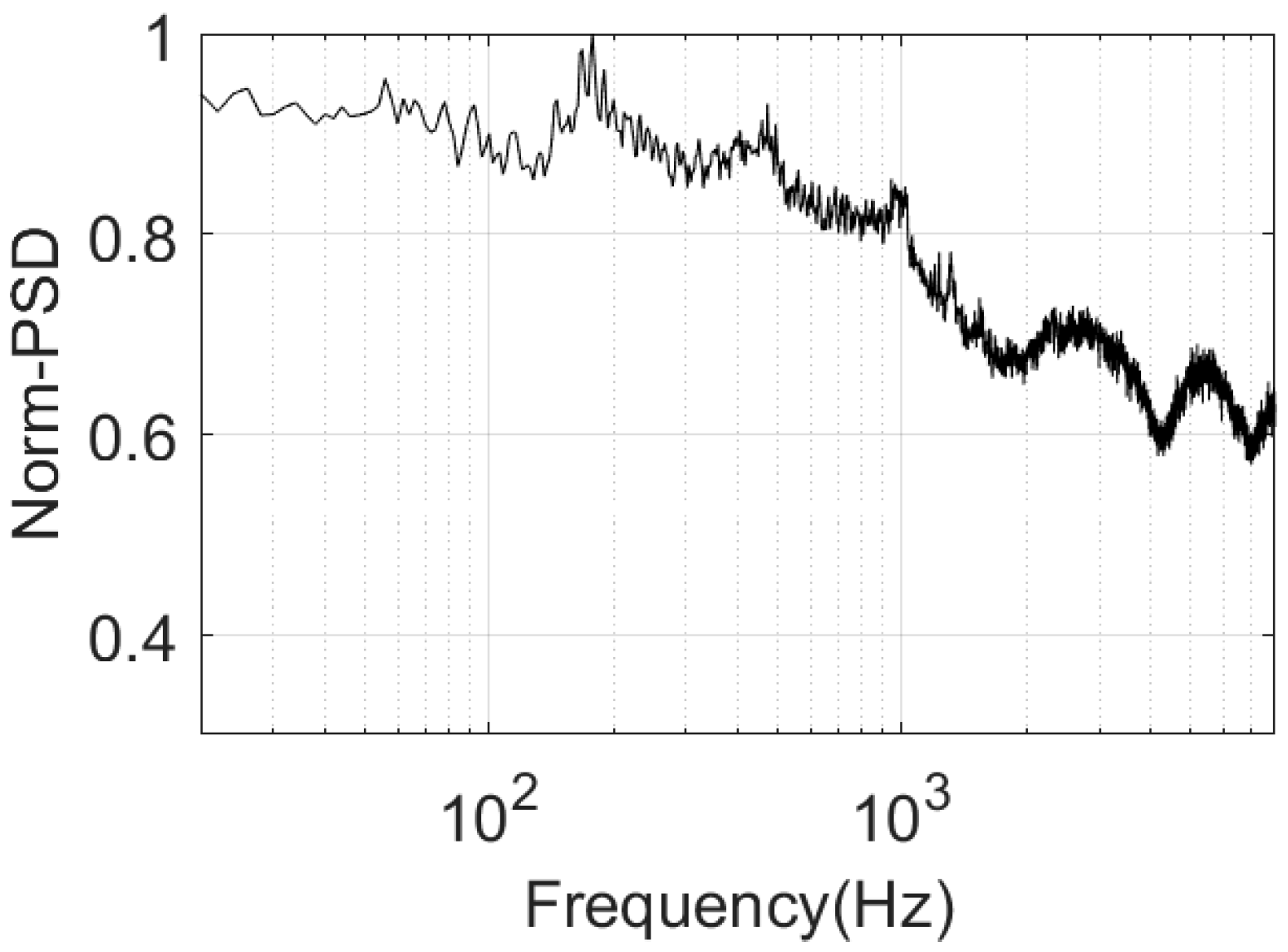
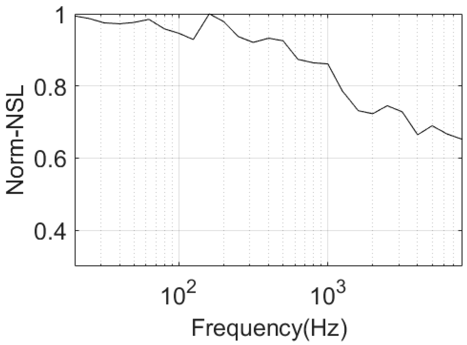
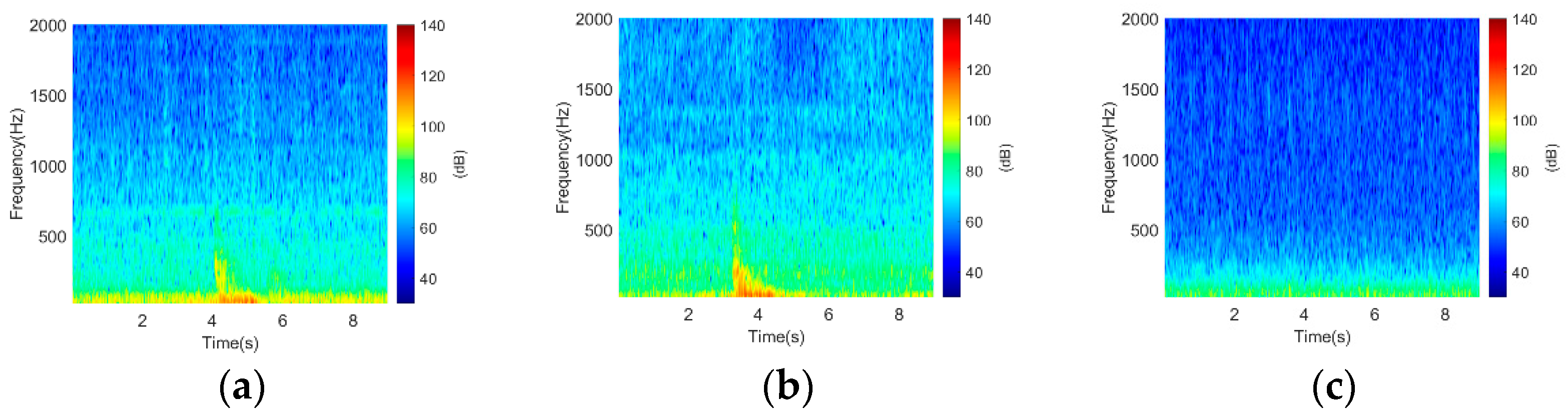
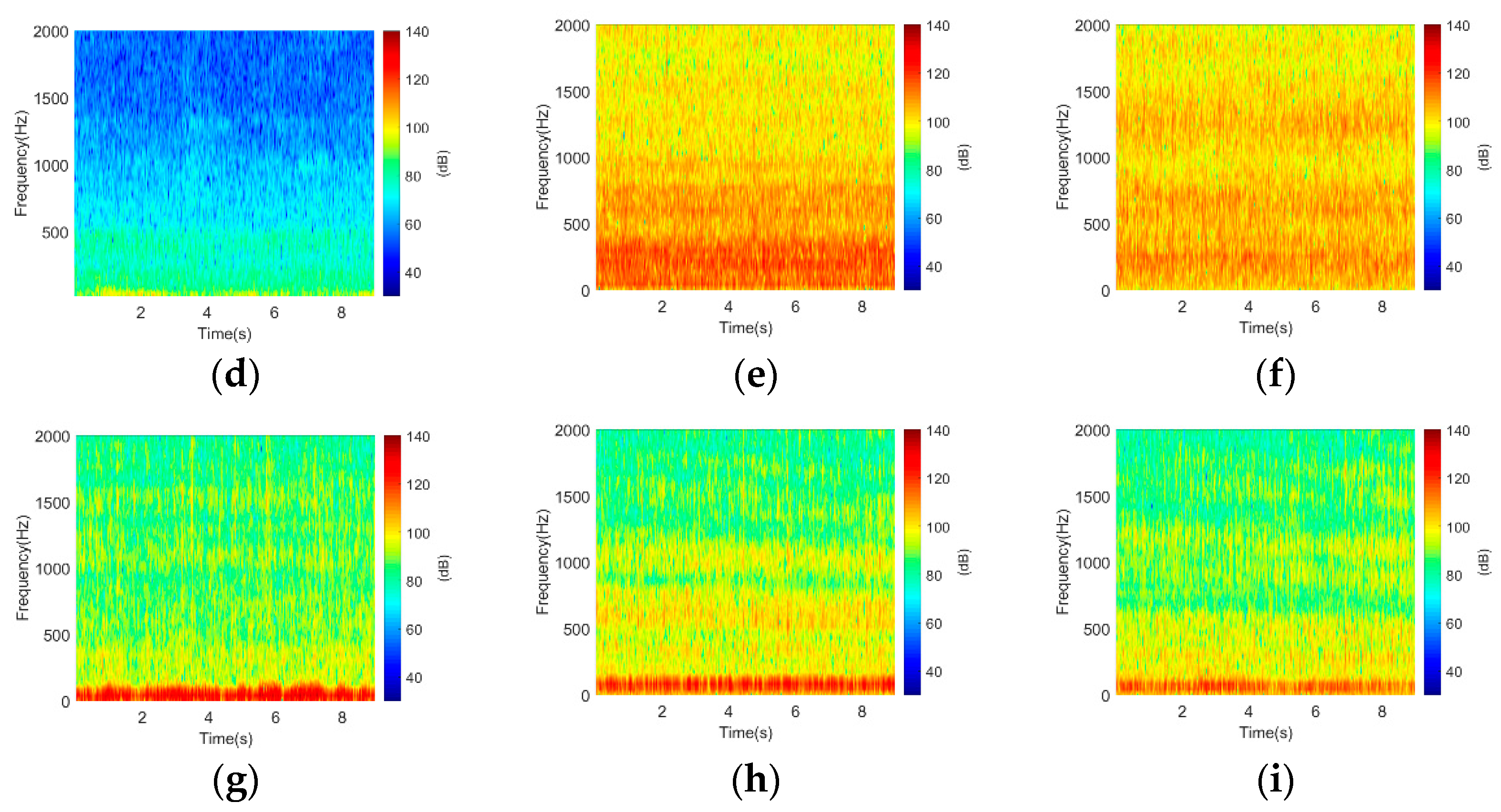
3.2.1. Underwater Noise Features Extraction

Because the UNGM primarily simulates the spectral characteristics of typical UN, the frequency domain characteristics are mainly extracted and used in classification.

• PSD.

The PSD is estimated using the average periodogram technique, with a Hamming window with a 50% overlap between adjacent frames. This analysis focuses on the frequency band of 20 Hz to 8 kHz with a frequency resolution of 2 Hz. This is because the lowest credible frequency of the noise recording system is 20 Hz, and although the highest frequency can be higher, the system above 8 kHz is subject to interference from bathymetric equipment. Correspondingly, the obtained PSD has 3991 frequency bins. To eliminate the effects of the absolute value of the PSD on the classification results, the PSD is normalized by its maximum value. Figure 5 shows the normalized PSD of a measured noise sample.

• 1/3 octave noise spectrum level (NSL).

The 1/3 octave NSL is a characteristic quantity commonly used to process UN data. Each obtained time-domain UN sequence is divided (using a sliding window) into $L$ data segments with a length of $N$, $x_i,i=1,2,\mathrm{\dots }L$. The 1/3 octave NSL is calculated for each data segment. The results for all $L$ data segments are summed and averaged.

Let $f_c$ be the central frequency, and $f_L=2^{-1/6}{f}_c$, $f_H=2^{1/6}{f}_c$ are the upper-limit frequency and lower-limit frequency of the 1/3 octave frequency band, $\Delta f=f_H-f_L$ is the bandwidth. Then, the average power of a continuous noise signal $x\left(t\right)$ with a duration of $\Delta T$ in the frequency band of $\Delta f$ is as follows:

$$\overline{I}(f_c)=\frac{1}{\Delta f}\frac{1}{\Delta T}\cdot 2\cdot {\displaystyle \underset{f_L}{\overset{f_H}{\int }}{\left|X\left(\omega \right)\right|}^2}df$$

(7)

Here, $X\left(\omega \right)$ is the Fourier transform (FT) of a finite continuous signal $x\left(t\right)$. Record $x\left(k\right)$ as the sampling sequence of $x\left(t\right)$, its discrete FT $X\left(k\right)$ is related to $X\left(\omega \right)$ though the following function,

$$X\left(\omega \right)=t_s\cdot X\left(k\right)$$

(8)

where $t_s$ is the sampling interval. Therefore, we have the following discrete form,

$$\overline{I}(f_c)=\frac{1}{\Delta f}\frac{1}{\Delta T}\cdot 2\cdot \frac{1}{N{f}_s}{\displaystyle \sum _{k=k_1}^{k=k_2}{\left|X\left(k\right)\right|}^2}$$

(9)

where $\Delta T=N{t}_s$, $f_L=(k_1-1)f_s/N$, and $f_H=(k_2-1)f_s/N$. Finally, the 1/3 octave noise spectrum level can be expressed as follows:

$$NSL=10\lg \left[\frac{1}{L}{\displaystyle \sum _{i=1}^L{\overline{I}}_i(f_c)}\right]-M-m$$

(10)

where $M$ is the sensitivity of the hydrophone and $m$ is the amplification factor of the amplifier.

In correspondence to the PSD, the 1/3 octave NSL in the frequency band of 20 Hz to 8 kHz is calculated. So, the ultimately obtained 1/3 octave NSL has 28 frequency bins. Similarly, the 1/3 octave NSL is normalized by the maximum value. Figure 6 shows the result obtained for the same noise sample as Figure 5.

It should be noted that because the PSD and NSL have different data dimensions, they are drawn as RGB images with a resolution of 32 × 32 pixels and three channels. Finally, each feature image is used as an input feature for UN classification.

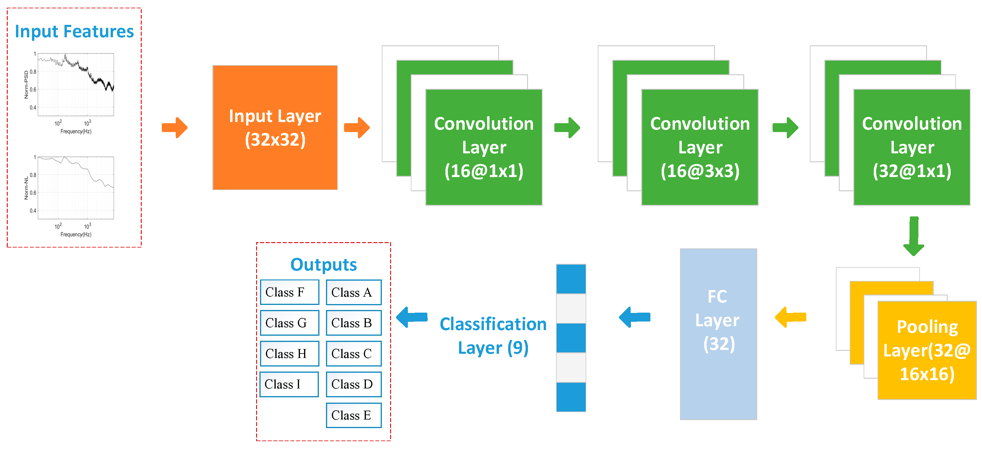
3.2.2. CNN Architecture Design

Inspired by classification tasks in the acoustic signal field [41,42,43], the CNN is designed as shown in Figure 7. It is composed of three convolutional layers: one pooling layer, one fully connected (FC) layer with 32 neurons, and a classification layer that assigns a score to each of the 9 classes.

The design follows two principles: (1) multiple layers of small convolution kernels are used to expand the receptive field and reduce the number of training parameters and overfitting; and (2) 1 × 1 convolutional layers are introduced as bottleneck layers to deepen the network while increasing or decreasing its dimensionality. Therefore, the first and third convolution layers adopted a 1 × 1 convolution kernel to include the bottleneck layer and increase the depth of the network, which is helpful for improving classification performance. Here, zero-padding is used to keep the numbers of input and output dimensions identical. Batch normalization and the rectified linear unit (ReLu) activation function are employed after each convolutional layer; this is a computationally efficient way to reduce the generalization error [44,45]. The pooling layer reduced the dimensionality based on the local correlation of the feature images using the max-pooling method with a pooling size and step of 2 × 2 and 2. Additionally, batch normalization was followed, which, on the one hand, accelerated the CNN’s training and, on the other hand, reduced the CNN’s sensitivity to network initialization and thus improved its generalization ability. The neural network was trained using the stochastic gradient descent method with a maximum number of training times of 20 and cross-entropy as the loss function.

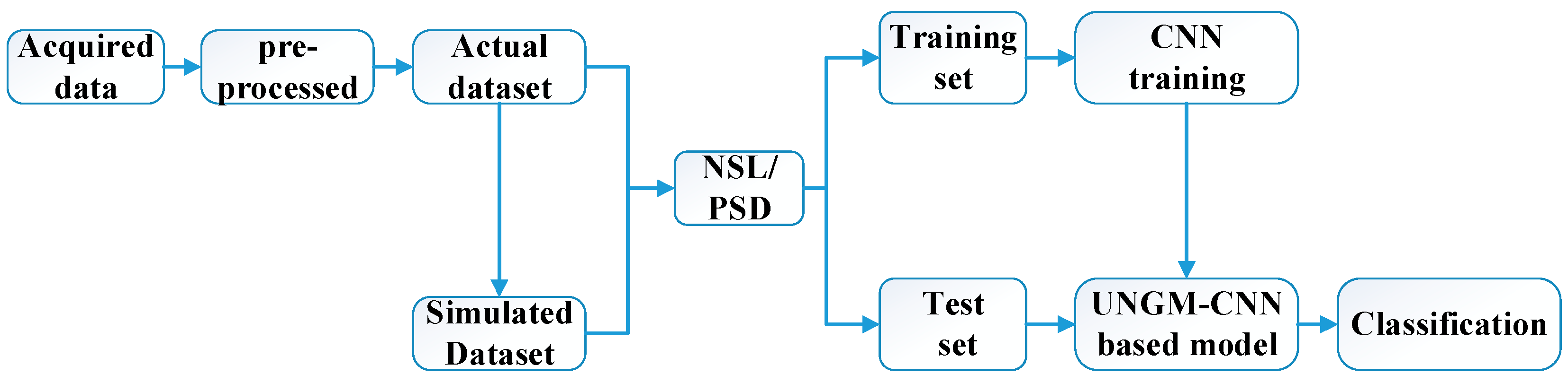
3.2.3. UNGM-CNN Based Classification Method

For the underwater noise measured, it is pre-processed to eliminate transient interference through empirical analysis and frequency spectrum analysis. Then the data were divided into equal lengths in the time domain to form the actual data, which includes N samples.

The UNGM is used to numerically simulate a sample for each of the experimentally measured UN samples. A total of N-simulated samples are obtained during each generation, and this process is performed 6 times. Several datasets are subsequently created. The measured data alone is the actual dataset. In addition, the measured data and simulated data yielded by different numbers of simulation processes are combined into different mixed sets.

Table 2. Details of dataset.

Dataset Name	Details of Dataset
Actual	Measured data
Simu	Simulated data yielded by one simulation process
Actual + 1 Simu	Measured data + simulated data yielded by one simulation process
Actual + 2 Simus	Measured data + simulated data yielded by two simulation processes
Actual + 6 Simus	Measured data + simulated data yielded by six simulation processes

summarizes the dataset types.

For all the samples in each dataset, the NSL and PSD features are extracted and normalized. Then the feature images are randomly grouped into five mutually disjoint subsets of the same size using the fivefold cross-validation method. Four of the five subsets are used to train the classification model, while the remaining subset is used to test the classification model. This process is repeated for all five possible combinations. Figure 8 shows the classification process. During the process, we refer to the method that only applies measured data as the CNN-based method and the method that uses a mixture of measured and simulated data as the UNGM-CNN-based method.

To evaluate the performance of the two methods, five metrics—accuracy, precision, recall, macro-precision, and macro-recall—are used. Accuracy is defined as the ratio of the number of samples that are correctly classified, $nu{m}_{ck}$, to the total number of samples tested, $nu{m}_{total}$, as follows:

$${\mathrm{Accuracy}}_{total}=1/5{\displaystyle {\sum }_{K=1}^5\frac{nu{m}_{ck}}{nu{m}_{total}}\cdot 100\%}$$

(11)

where $K$ is the number of cross-validations.

Precision is the ratio of the number of samples that are correctly classified as samples for a given type of UN to the total number of samples that are predicted to be samples for this type of UN, as follows:

$$\mathrm{Precision}=\frac{nu{m}_{TruePositives}}{nu{m}_{TruePositives}+nu{m}_{FalsePositives}}\cdot 100\%$$

(12)

Recall is the ratio of the number of samples that are correctly classified as samples for a given type of UN to the total number of samples for this type of UN, as follows:

$$\mathrm{Recall}=\frac{nu{m}_{TruePositives}}{nu{m}_{TruePositives}+nu{m}_{FalseNegatives}}\cdot 100\%$$

(13)

Macro-precision is defined as the precision averaged across all types, as follows:

$$\mathrm{Macro-Precision}={\displaystyle \sum _{i=1}^N\mathrm{P}{\mathrm{recision}}_i}$$

(14)

Macro-recall is defined as the recall averaged across all types, as follows:

$$\mathrm{Macro-Recall}={\displaystyle \sum _{i=1}^N\mathrm{R}{\mathrm{ecall}}_i}$$

(15)

where $N$ is the number of types. A high precision indicates a low false-positive rate, while a high recall suggests a high true-positive rate.

4. Experiments and Discussions

4.1. Experimental Data and Labeling Related Work

The underwater noise data were collected from three noise measurement experiments and were divided into 9 classes according to the main noise sources.

• A. Shallow sea experiment in the northern South China Sea (SCS).

A single-point noise-measuring hydrophone (sensitivity: −164 dB) was lowered to the floor of the SCS to collect noise data at a sampling frequency of 24 kHz. During some periods of time during this noise measurement experiment, ship-radiated noise was also measured. The participating fishing vessels traveled back and forth at a speed of 5 to 9 knots in the vicinity of the hydrophone. The distance between the vessel and the hydrophone varied from approximately 0.1 to 2.0 km. This experiment was intermittently affected by the noise emitted from the air gun onboard a drillship in the SCS. The air gun emitted a signal every 9 s, which lasted for approximately 1.5 s. Therefore, three types of noise from different main sources were sampled and labeled. They were single-vessel noise (labeled as KeDiao), air-gun noise (labeled as AirGun), and mixed air-gun and vessel noise (labeled as AirKeD). The duration of the samples was 9 s.

• B. Deep sea experiment in the northern SCS.

A subsurface buoy (sensitivity: −166 dB) was used to collect the ambient noise (labeled as AmbNoi) from the deep waters of the SCS at a depth of 4250 m with a sampling frequency of 64 kHz. Similarly, the duration of the samples was 9 s.

• C. Experiment in the East China Sea (ECS).

A hydrophone was lowered to a depth of approximately 7 m to collect ship-radiated noise in the coastal waters of the ECS at a frequency of 44.1 kHz. Noise data for five fishing vessels were collected separately, which were labeled FisherA, FisherB, FisherC, FisherD, and FisherE.

It should be noted that all data were down-sampled to 20 kHz. This is because we think that the characteristic differences between different dominant noise sources are mainly concentrated in the frequency band below 10 kHz. On the other hand, since sample features will be normalized, environmental information such as hydrology and topography is not considered.

Therefore, 9 classes of noise are acquired. Figure 9 shows the time-frequency spectrum of each noise (in the 20 Hz to 2 kHz frequency band only). The color in the figure represents the strength of energy. The red part below 500 Hz in (a) and (b) means the airgun. Analysis reveals a high level of similarity between the AirGun noise and the AirKeD noise; they are easy to confuse with the naked eye. Figure 9c shows typical ocean background noise without any obvious interference. Figure 9d–i represents different ships. The line spectrum that runs through the entire time is a typical feature of ship noise. This also increases the difficulty of classification to some extent because different ships can be similar, just like FisherD and FisherE.

Table 3. General information on 9 types of typical UN.

Main Noise Source	Air-Gun Noise	Mixed Air-Gun and Vessel Noise	Ambient Noise	KeDiao Vessel	Fishing Vessel A	Fishing Vessel B	Fishing Vessel C	Fishing Vessel D	Fishing Vessel E
label	AirGun	AirKeD	AmbNoi	KeDiao	FisherA	FisherB	FisherC	FisherD	FisherE
sample size	200	300	210	300	200	300	300	200	190

shows the details of the 9 types of underwater noise. There are 190 to 300 samples for each type. A total of 2200 samples are used for analysis. Therefore, combined with the simulated data samples, the final datasets are shown in

Table 4. Dataset types and their sample sizes.

Dataset Name	Dataset Size	Training Dataset	Test Dataset
Actual	2200	1760	440
Simu	2200	--	--
Actual + 1 Simu	4400 (2200 + 2200)	3520	880
Actual + 2 Simus	6600 (2200 + 2200 × 2)	5280	1320
Actual + 6 Simus	15,400 (2200 + 2200 × 6)	12,320	3080

.

It should be noted that the numbers of samples for each type of UN in the training and test sets generated are random.

Table 5. Number of samples for each type of UN in the training set created from the measured data set at the Kth cross-validation.

K-Fold	AirGun	AirKeD	AmbNoi	KeDiao	FisherA	FisherB	FisherC	FisherD	FisherE	Total
K = 1	41	44	33	65	51	70	52	42	42	440
K = 2	37	70	46	56	39	68	57	32	35	440
K = 3	40	63	43	55	38	62	59	49	31	440
K = 4	44	60	40	52	41	73	56	37	37	440
K = 5	38	69	49	59	34	44	65	41	41	440

summarizes the number of samples for each type of UN in the training set created from the measured dataset at the Kth cross-validation.

4.2. Discussions

Firstly, compare the performance of the two methods. In Figure 10, the red bar represents the CNN-based method, while the blue bar represents the UNGM-CNN-based method using the Actual + 6 Simus dataset. Overall, when NSL is the input feature, the CNN-based method achieves an accuracy of 98.27%, while the UNGM-CNN-based method achieves a 99.86% accuracy. When PSD is the input feature, the accuracies of the two methods are 97.45% and 99.89%, respectively. That is to say, the UNGM-CNN-based method increases the classification accuracy by 1.59% and 2.44% compared to the CNN-based method when NSL and PSD are used as the input features, respectively.

Then compare the effect of dataset size on the UNGM-CNN-based method, as shown in Figure 11. Here, the pink line and blue line represent the cases where NSL and PSD are input features, respectively. Observation of the trend of the two lines reveals that augmenting the dataset can gradually improve the classification performance. This further demonstrates the advantages of the UNGM-CNN-based method over the CNN-based method.

Table 6. Test results obtained of CNN-based method (K = 1).

		Predicted Class
		AirGun	AirKeD	AmbNoi	KeDiao	FisherA	FisherB	FisherC	FisherD	FisherE	Recall
True Class	AirGun	39	1	0	1	0	0	0	0	0	95.12%
	AirKeD	1	43	0	0	0	0	0	0	0	97.73%
	AmbNoi	0	0	33	0	0	0	0	0	0	100%
	KeDiao	0	2	0	63	0	0	0	0	0	96.92%
	FisherA	0	0	0	0	51	0	0	0	0	100%
	FisherB	0	0	0	0	0	70	0	0	0	100%
	FisherC	0	0	0	0	0	0	52	0	0	100%
	FisherD	0	0	0	0	0	0	0	42	0	100%
	FisherE	0	0	0	0	0	0	0	0	42	95.12%
	Precision	97.50%	93.48%	100%	98.44%	100%	100%	100%	100%	100%	--

and

Table 7. Test results obtained of UNGM-CNN-based method (K = 1).

		Predicted Class
		AirGun	AirKeD	AmbNoi	KeDiao	FisherA	FisherB	FisherC	FisherD	FisherE	Recall
True Class	AirGun	288	0	0	0	0	0	0	0	0	100%
	AirKeD	1	412	0	1	0	0	0	0	0	99.52%
	AmbNoi	0	0	310	0	0	0	0	0	0	100%
	KeDiao	0	0	0	411	0	0	0	0	1	99.76%
	FisherA	0	0	0	0	270	2	0	0	0	99.26%
	FisherB	0	0	0	0	0	405	0	0	0	100%
	FisherC	0	1	0	0	0	0	417	0	0	99.76%
	FisherD	0	0	0	0	0	0	0	282	2	99.30%
	FisherE	0	0	0	0	0	0	0	1	276	99.64%
	Precision	99.65%	99.76%	100%	99.76%	100%	99.51%	100%	99.65%	98.92%	--

summarize the test results for the CNN-based method and the UNGM-CNN-based method with 6 times simulated data. The input feature is NSL. In Table 6, the classifier is highly susceptible to mistaking UN samples of three types, AirGun, AirKeD, and KeDiao, which results in low precision and recall for each of them. The primary cause of this unsatisfactory performance of the classifier is that AirKeD is a mixture of AirGun and KeDiao. And this is also a challenge to the classification process. In Table 7, the precision of the 3 types is enhanced to greater than 99%. This is another advantage of the UNGM-CNN-based method.

The precision and recall of each type of noise are shown in Figure 12 and Figure 13. Overall, the precision of the UNGM-CNN-based method is better than that of the CNN-based method, with relatively low accuracy in the three categories of FisherB, FisherD, and FisherE, which are 0.49%, 0.35%, and 1.08% lower, respectively. But for the classes of AirGun, AirKeD, and KeDiao, the precisions are 2.15%, 6.28%, and 1.32% higher. The results of recall are similar to precision, with slightly lower recall in FisherA, FisherC, and FisherD and higher results in the other 6 classes. For example, they are 4.88%, 1.79%, 2.84%, and 4.52% higher than the CNN-based method in the AirGun, AirKeD, KeDiao, and FisherE, respectively.

Obviously, the UNGM-CNN-based method performs far superior to the CNN-based method in the three categories of AirGun, AirKeD, and KeDiao. We found that since AirKeD is a mixture of AirGun and KeDiao, more data is needed to extract feature differences between different categories. The UNGM-CNN-based method just meets this point. As for the reasons for the slightly poor performance in some ships, we think that this is caused by the error between the noise generated data and the real data. During the simulation process, the line spectrum of ships may not be perfectly simulated.

Based on Table 6 and Table 7, the macro-precision and macro-recall of the CNN-based method and the UNGM-CNN-based method are obtained, as shown in

Table 8. Comparison of the macro-precision and macro-recall.

	CNN-Based Method	UNGM-CNN-Based Method
Micro-precision	98.82%	99.69%
Micro-recall	98.86%	99.69%

. Evidently, the new method increases both macro-precision and macro-recall, specifically by approximately 0.87% and 0.83%, as compared to those of the old method.

In a word, the comparison of accuracy, precision, recall, macro-precision, and macro-recall between the two methods indicates that the UNGM-CNN-based method can improve the classification performance. The accuracy is 1.59% and 2.44% higher than the CNN-based method when NSL and PSD are used as the input features, respectively. Overall, the precision and recall are better than with the old method. The UNGM-CNN-based method performs far better than the CNN-based method in the three categories of AirGun, AirKeD, and KeDiao. And the macro-precision and macro-recall increase specifically by approximately 0.87% and 0.83% as compared to those of the old method.

5. Conclusions

This study focuses on addressing the problem of small sample sizes associated with UN classification. Specifically, a generative underwater noise model is established by white noise generation and filter design. From it, underwater noise can be simulated with a desired power spectral density and kurtosis. Therefore, it can be employed to augment measured data, such as the nine types of typical UN, including AirGun, AirKeD, AmbNoi, KeDiao, and five fishing vessels. Then, a UNGM-CNN-based underwater noise classification model is established. Results reveal that: (1) The CNN-based noise classification model is effective in classifying the nine types of underwater noise. For the measured data, it can get an accuracy of 98.27% and 97.45% when NSL and PSD are feature inputs, respectively. (2) The UNGM-CNN-based method performs better than the CNN-based method. Regardless of whether the NSL or PSD is used as the input feature, it can achieve a classification accuracy higher than 99.86%. The accuracy increases by 1.59% and 2.44% when the NSL and PSD are used as the input features with 6 times simulated data, respectively. Additionally, the UNGM-CNN-based method appreciably increases the macro-precision and macro-recall by approximately 0.87% and 0.83%, respectively. These findings lend credence to the effectiveness of the UNGM established in this study in noise classification involving small sample sizes. The methodology used in this work can be easily generalized to other passive acoustic sound classification problems. An efficient classification system like this can be of great help in identifying ships as well as other vehicles. Moreover, it will be helpful to marine oncologists in ensuring a marine habitat-friendly, noise-free ocean environment.

References

1. Garcia-Garcia, A.; Orts-Escolano, S.; Oprea, S. A survey on deep learning techniques for image and video semantic segmentation. Appl. Soft Comput. 2018, 70, 41–65. [Google Scholar] [CrossRef]
2. Li, X.; Long, S.; Zhu, J. Survey of few-shot learning based on deep neural network. Appl. Res. Comput. 2020, 37, 2241–2247. [Google Scholar]
3. Liu, Y.; Lei, Y.; Fan, J.; Wang, F.; Gong, Y.; Tian, Q. Survey of few-shot learning based on deep neural network. Surv. Image Classif. Technol. Based Small Sample Learn. 2021, 47, 297–315. [Google Scholar]
4. Zhang, R.; Che, T.; Ghahramani, Z. MetaGAN: An adversarial approach to few-shot learning. In Proceedings of the 32nd International Conference on Neural Information Processing Systems, Montreal, QC, Canada, 2–8 December 2018. [Google Scholar]
5. Zhao, K.; Jin, X.; Wang, Y. Survey on few-shot learning. J. Softw. 2021, 32, 349–369. [Google Scholar]
6. Dixit, M.; Kwitt, R.; Niethammer, M.; Vasconcelos, N. AGA: Attribute guided augmentation. In Proceedings of the IEEE Conference on Computer Vision and Pattern Recognition, Honolulu, HI, USA, 21–26 July 2017; pp. 7455–7463. [Google Scholar]
7. Liu, B.; Wang, X.; Dixit, M.; Kwitt, R.; Vasconcelos, N. Feature space transfer for data augmentation. In Proceedings of the IEEE Conference on Computer Vision and Pattern Recognition, Salt Lake City, UT, USA, 18–22 June 2018; pp. 9090–9098. [Google Scholar]
8. Long, M.; Cao, Y.; Wang, J.; Jordan, M.I. Learning transferable features with deep adaptation networks. In Proceedings of the 32nd International Conference on Machine Learning, Lille, France, 6–11 July 2015; pp. 97–105. [Google Scholar]
9. Qi, H.; Brown, M.; Lowe, D.G. Low-shot learning with imprinted weights. In Proceedings of the 2018 IEEE/CVF Conference on Computer Vision and Pattern Recognition, Salt Lake City, UT, USA, 18–22 June 2018; pp. 5822–5830. [Google Scholar]
10. Koch, G.; Zemel, R.; Salakhutdinov, R. Siamese neural networks for one-shot image recognition. In Proceedings of the 32nd International Conference on Machine Learning, Lille, France, 6–11 July 2015. [Google Scholar]
11. Zhou, L.J.; Cui, P.; Yang, S.Q.; Zhu, W.W.; Tian, Q. Learning to learn image classifiers with informative visual analogy. In Proceedings of the 2019 IEEE/CVF Conference on Computer Vision and Pattern Recognition, Long Beach, CA, USA, 15–20 June 2019. [Google Scholar]
12. Ravi, S.; Larochelle, H. Optimization as a model for few-shot learning. In Proceedings of the ICLR—International Conference on Learning Representations, San Juan, Puerto Rico, 2–4 May 2016. [Google Scholar]
13. Wang, X.; Yu, F.; Wang, R.; Darrell, T.; Gonzalez, J.E. TAFE-Net: Task-aware feature embeddings for low shot learning. In Proceedings of the IEEE Conference on Computer Vision and Pattern Recognition, Long Beach, CA, USA, 15–20 June 2019; pp. 1831–1840. [Google Scholar]
14. Gidaris, S.; Komodakis, N. Dynamic few-shot visual learning without forgetting. In Proceedings of the IEEE Conference on Computer Vision and Pattern Recognition, Salt Lake City, UT, USA, 18–22 June 2018; pp. 4367–4375. [Google Scholar]
15. Yang, H.; Li, J.; Shen, S.; Xu, G. A deep convolutional neural network inspired by auditory perception or underwater acoustic target recognition. Sensors 2019, 19, 1104. [Google Scholar] [CrossRef] [PubMed] [Green Version]
16. Ozanich, E.; Gerstoft, E.P.; Niu, H. A feedforward neural network for direction-of-arrival estimation. J. Acoust. Soc. Am. 2020, 147, 2035–2048. [Google Scholar] [CrossRef]
17. Niu, H.; Gong, Z.; Ozanich, E.; Gerstoft, P.; Wang, H.; Li, Z. Deep learning source localization using multi-frequency magnitude-only data. J. Acoust. Soc. Am. 2019, 146, 211–222. [Google Scholar] [CrossRef] [Green Version]
18. Van Komen, D.F.; Neilsen, T.B.K.; Howarth, K.; Knobles, D.P.; Dahl, P.H. Seabed and range estimation of impulsive time series using a convolutional neural network. J. Acoust. Soc. Am. 2020, 147, EL403–EL408. [Google Scholar] [CrossRef]
19. Song, G.; Guo, X.; Wang, W.; Li, J.; Yang, H.; Ma, L. Underwater Noise Classification based on Support Vector Machine. In Proceedings of the IEEE/OES China Ocean Acoustics Conference COA 2021, Harbin, China, 14–17 July 2021. [Google Scholar]
20. Lăzăroiu, G.; Andronie, M.; Iatagan, M.; Geamănu, M.; Ștefănescu, R.; Dijmărescu, I. Deep Learning-Assisted Smart Process Planning, Robotic Wireless Sensor Networks, and Geospatial Big Data Management Algorithms in the Internet of Manufacturing Things. ISPRS Int. J. Geo-Inf. 2022, 11, 277. [Google Scholar] [CrossRef]
21. Blake, R.; Frajtova Michalikova, K. Deep Learning-based Sensing Technologies, Artificial Intelligence-based Decision-Making Algorithms, and Big Geospatial Data Analytics in Cognitive Internet of Things. Anal. Metaphys. 2021, 20, 159–173. [Google Scholar]
22. Andronie, M.; Lăzăroiu, G.; Iatagan, M.; Hurloiu, I.; Ștefănescu, R.; Dijmărescu, A.; Dijmărescu, I. Big Data Management Algorithms, Deep Learning-Based Object Detection Technologies, and Geospatial Simulation and Sensor Fusion Tools in the Internet of Robotic Things. ISPRS Int. J. Geo-Inf. 2023, 12, 35. [Google Scholar] [CrossRef]
23. Li, C.; Huang, Z.; Xu, J.; Guo, X.; Gong, Z.; Yan, Y. Multi-channel underwater target recognition using deep learning. Acta Acust. 2020, 45, 506–514. [Google Scholar]
24. Wang, W.; Ni, H.; Su, L. Deep transfer learning for source ranging: Deep-sea experiment results. J. Acoust. Soc. Am. 2019, 146, EL317–EL322. [Google Scholar] [CrossRef] [Green Version]
25. Escobar-Amado, C.D.; Badiey, M.; Pecknold, S. Automatic detection and classification of bearded seal vocalizations in the northeastern Chukchi Sea using convolutional neural networks. J. Acoust. Soc. Am. 2022, 151, 299–309. [Google Scholar] [CrossRef]
26. Zhong, M.; Castellote, M.; Dodhia, R. Beluga whale acoustic signal classification using deep learning neural network models. J. Acoust. Soc. Am. 2020, 147, 1834–1841. [Google Scholar] [CrossRef]
27. Li, X.; Song, W.; Gao, D.; Gao, W.; Wang, H. Training a U-Net based on a random mode-coupling matrix model to recover acoustic interference striations. J. Acoust. Soc. Am. 2020, 147, EL362–EL369. [Google Scholar] [CrossRef] [Green Version]
28. Ekpezu, A.O.; Wiafe, I.; Katsriku, F.; Yaokumah, W. Using deep learning for acoustic event classification: The case of natural disasters. J. Acoust. Soc. Am. 2021, 149, 2926–2935. [Google Scholar] [CrossRef]
29. Escobar-Amado, C.D.; Neilsen, T.B.; Castro-Correa, J.A.; Van Komen, D.F.; Badiey, M.; Knobles, D.P.; Hodgkiss, W.S. Seabed classification from merchant ship-radiated noise using a physics-based ensemble of deep learning algorithms. J. Acoust. Soc. Am. 2021, 150, 1434–1447. [Google Scholar] [CrossRef] [PubMed]
30. Zhong, M.; Maelle, T.; Trevor, A.B.; Kathleen, M.S.; Jean-Yves, R.; Rahul, D.; Juan, L.F. Detecting, classifying, and counting blue whale calls with Siamese neural network. J. Acoust. Soc. Am. 2021, 149, 3086–3094. [Google Scholar] [CrossRef]
31. Wu, G.; Li, J.; Li, X.; Chen, Y.; Yuan, Y. Ship radiated-noise recognition (IV)-recognition using fuzzy neural network. Acta Acust. 1999, 24, 275–280. [Google Scholar]
32. Wu, Y.; Yang, L. Ship image classification by combined use of HOG and SVM. J. Shanghai Ship Shipp. Res. Inst. 2019, 42, 58–64. [Google Scholar]
33. Yang, K.; Zhou, X. Deep learning classification for improved bicoherence feature based on cyclic modulation and cross-correlation. J. Acoust. Soc. Am. 2019, 146, 2201–2211. [Google Scholar] [CrossRef]
34. Premus, V.E.; Evans, M.E.; Abbot, P.A. Machine learning-based classification of recreational fishing vessel kinematics from broadband striation patterns. J. Acoust. Soc. Am. 2020, 147, EL184–EL188. [Google Scholar] [CrossRef] [Green Version]
35. Song, G.; Guo, X.; Wang, W. A machine learning-based underwater noise classification method. Appl. Acoust. 2021, 184, 10833. [Google Scholar] [CrossRef]
36. Mishachandar, B.; Vairamuthua, S. Diverse ocean noise classification using deep learning. Appl. Acoust. 2021, 181, 108141. [Google Scholar] [CrossRef]
37. Webster, R.J. A random number generator for ocean noise statistics. IEEE J. Ocean. Eng. 1994, 19, 134–137. [Google Scholar] [CrossRef]
38. Webster, R.J. Ambient noise statistics. IEEE Trans. Signal Pro. 1993, 41, 2249–2253. [Google Scholar] [CrossRef]
39. Dolan, B.A. The Mellin transform for moment generation and for the probability density of products and quotients of random variables. Proc. IEEE 1964, 52, 1745–1746. [Google Scholar] [CrossRef]
40. Song, G.; Guo, X.; Ma, L.; Li, H. Non-Gaussian Ocean Ambient Noise Model with Certain Kurtosis. Chin. J. Acoust. 2020, 39, 498–511. [Google Scholar]
41. Neilsen, T.B.; Escobar-Amado, C.D.; Acree, M.C.; Hodgkiss, W.S.; Van Komen, D.F.; Knobles, D.P.; Badiey, M. Learning location and seabed type from a moving mid-frequency source. J. Acoust. Soc. Am. 2021, 149, 692–705. [Google Scholar] [CrossRef] [PubMed]
42. Frederick, C.; Villar, S.; Michalopoulou, Z.H. Seabed classification using physics-based modeling and machine learning. J. Acoust. Soc. Am. 2020, 148, 859–872. [Google Scholar] [CrossRef] [PubMed]
43. Bianco, M.J.; Gerstoft, P.; Traer, J.; Ozanich, E.; Roch, M.A.; Gannot, S.; Deledalle, C.A. Machine learning in acoustics: Theory and applications. J. Acoust. Soc. Am. 2019, 146, 3590–3628. [Google Scholar] [CrossRef] [PubMed] [Green Version]
44. Nair, V.; Hinton, G.E. Rectified Linear Units Improve Restricted Boltzmann Machines. In Proceedings of the 27th International Conference on Machine Learning (ICML-10), Haifa, Israel, 21–24 June 2010. [Google Scholar]
45. Ioffe, S.; Szegedy, C. Batch normalization: Accelerating deep network training by reducing internal covariate shift. In Proceedings of the 32nd International Conference on Machine Learning, Lille, France, 6–11 July 2015. [Google Scholar]
Figure 1. Framework of the proposed method.
Electronics 12 02669 g001
Figure 2. Flow chart of underwater noise generation.
Electronics 12 02669 g002
Figure 3. Normalized PSDs of the numerically simulated and measured samples.
Electronics 12 02669 g003
Figure 4. Kurtosis of numerically simulated and measured samples.
Electronics 12 02669 g004
Figure 5. Normalized PSD of a sample.
Electronics 12 02669 g005
Figure 6. The 1/3 octave NSL of a sample.
Electronics 12 02669 g006
Figure 7. CNN architecture for underwater noise classification.
Electronics 12 02669 g007
Figure 8. UNGM-CNN-based underwater noise classification method.
Electronics 12 02669 g008
Figure 9. Spectrograms of the 9 types of noise. (a) AirGun; (b) AirKeD; (c) AmbNoi; (d) KeDiao; (e) FisherA; (f) FisherB; (g) FisherC; (h) FisherD; (i) FisherE.
Electronics 12 02669 g009aElectronics 12 02669 g009b
Figure 10. Comparison of CNN-based and UNGM-CNN-based methods.
Electronics 12 02669 g010
Figure 11. Effects of dataset size of UNGM-CNN-based method.
Electronics 12 02669 g011
Figure 12. Precision of each class of UNGM-CNN-based method.
Electronics 12 02669 g012
Figure 13. Recall of each class of UNGM-CNN-based method.
Electronics 12 02669 g013