1. Introduction
Simultaneous localization and mapping (SLAM) technology plays a critical role in perception-based supporting path planning, obstacle avoidance, and other practical applications in autonomous robot navigation. In recent years, LiDAR–inertial SLAM systems have demonstrated higher accuracy and stronger environmental adaptability than systems based on single-type sensors [
1].
Currently, classic algorithms for LiDAR–inertial SLAM are mainly represented by loosely coupled LiDAR odometry and mapping (LOAM) [
2] and tightly coupled Laser–inertial odometry and mapping (LIOM) [
3]. However, using LiDAR as the primary sensor presents certain limitations because LiDAR–inertial SLAM heavily relies on the quality of the point cloud data obtained from LiDAR. In sparsely structured scenarios with geometrically repetitive patterns, certain directional constraints may be missing, making it difficult to estimate motion in certain degrees of freedom. This can result in degenerate accuracy or even failure of the SLAM system. In scenes with unidirectional sparse structures such as long tunnels, single-sided walls, and bridges, laser matching has an additional degree of freedom in one direction. When moving forward along a tunnel, the acquired laser point cloud is the same, making it difficult for the matching algorithm to accurately estimate the motion in this direction. Similarly, this situation occurs when the machine moves around a cylindrical object in a circle. In scenarios featuring unidirectional sparse structures such as lengthy tunnels, walls on a single side, and bridges, laser matching encounters an additional challenge regarding motion estimation in one particular direction. Specifically, when progressing forward along a tunnel, the gathered laser point cloud remains unchanged, creating difficulties for the matching algorithm in accurately estimating the motion in that specific direction. Likewise, a similar circumstance arises when the machine circumnavigates a cylindrical object in a circular path. In multidirectional sparsely structured scenarios such as plazas or airports, using only ground point clouds for matching may lack constraints from surrounding directions, leading to drift and random variations in the odometry. These issues can result in deteriorating drift correction and a significant cumulative error over time.
As intelligent mobile platforms are being increasingly deployed in diverse scenarios, SLAM systems are required to deliver higher levels of precision and robustness. Masaki et al. proposed a method that utilizes the Fisher information matrix to determine the level of degeneracy. By redefining the Fisher matrix based on the robot’s motion state information, the reliability of the robot’s localization on a known map can be assessed by analyzing the matrix’s eigenvalues [
4]. Ji Zhang et al. designed degeneracy factors to characterize the level of degeneracy in each direction for optimization-based state estimation [
5]. Additionally, due to the inherent difficulty faced by LiDAR in overcoming degeneracy in scenarios with sparse structures, solely relying on LiDAR and inertial information may not be sufficient to correct errors. To improve SLAM performance in degenerate environments, multiple-sensor fusion is commonly adopted to provide additional constraints for pose estimation, compensating for the inherent lack of constraints of LiDAR.
Weizhao Shao et al. proposed variational inference learning-based simultaneous localization and mapping (VIL–SLAM), which utilizes tightly coupled visual–inertial odometry as prior information to aid LiDAR-based SLAM and further improves LiDAR information with visual-LiDAR loop closure detection [
6]. However, this method still has shortcomings in terms of system complexity and potential losses. Weikun Zhen et al. evaluated the performance of LiDAR-based localization by comparing the constrained equations after perturbation. They proposed an ESKF-based LiDAR–inertial navigation SLAM fused with ultra-wide band (UWB) information, providing valuable insights for multisensor fusion solutions [
7].
To address the issue of the poor performance of LiDAR–inertial SLAM in degenerate environments, this paper proposes a LiDAR–inertial SLAM method based on a virtual inertial navigation system to provide additional constraints during free direction. This approach uses a convolutional neural network (CNN) with attention mechanisms to classify robot torso IMU information corresponding to each gait. Then, a residual network–gated recurrent unit (ResNet–GRU) hybrid model is employed to extract the nonlinear mapping relationship between the torso and foot IMU information and construct the virtual IMU and VINS corresponding to each gait. A zero-velocity update is applied to estimate and correct the position, velocity, pose error, and virtual IMU errors in real time. The corrected pose information is then input into the LiDAR–inertial odometry calculation process to maintain the odometry’s accuracy over short periods. When the robot operates in degenerate environments where its mapping and localization performance is reduced, the VINS system can assist in correcting the robot’s estimated state parameters to optimize the accuracy of the constructed map.
2. System Overview
This paper proposes a method for LiDAR–inertial SLAM based on a virtual inertial navigation system to address the navigation problem of degeneracy with quadruped robots.
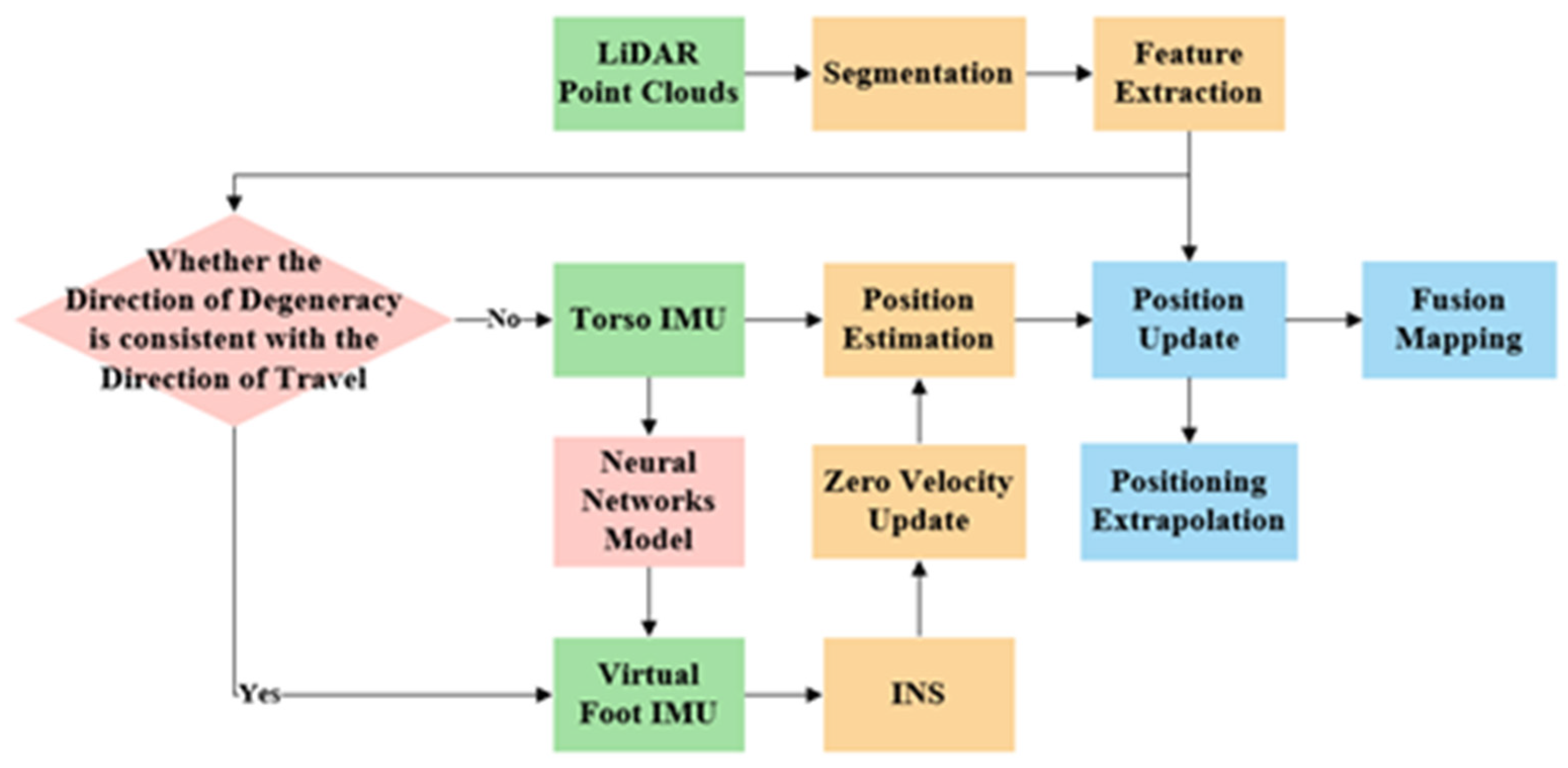
Figure 1 shows the detailed implementation process. The proposed LiDAR–inertial SLAM method based on VINS was designed with a convolutional neural network (CNN) model based on the attention mechanism trained to classify the robot’s motion patterns. This model is used to build corresponding models for each gait. The torso IMU data are classified into different gaits, and the relationship between the torso IMU data and foot IMU data is modeled using a ResNet–GRU hybrid network to build a virtual foot IMU for each gait. The virtual inertial information from the torso IMU mapped to the foot, along with the collected inertial information from the torso, is processed by an inertial navigation algorithm with a zero-velocity update to calculate the robot’s pose. The algorithm then outputs the pose estimation. This approach eliminates the need to install inertial sensors on the feet of the robot during navigation.
Following timestamp alignment, the missing pose data that are not from laser scan matching are inferred by means of timestamps and other LiDAR data. Both are continuously updated and initialized to minimize the errors accumulated during the pose fusion step. All data are then cached; the algorithm constantly polls and optimizes the fused pose, IMU data, and odometer data, updating these three data based on virtual IMU data. Ultimately, the fused pose is obtained to complete the localization and mapping process.
Based on the constructed LiDAR constraints equation, the system constraint weight is evaluated to calculate the degenerate direction. If the locomotion direction of the quadrupedal robot aligns with the environment’s degenerate direction, or when the reliability of the LiDAR localization information gradually decreases, the performance of the LiDAR–inertial navigation system is deemed to be insufficient, and the system transitions to a SLAM solution assisted by a VINS to continue operation. Otherwise, if the LiDAR–inertial navigation system operates normally, the computation of the virtual inertial information is not activated, and the system state remains unchanged, referring to LINS.
When the VINS is activated, feature points are extracted through curvature calculation, and the distortion caused by uniform motion is removed during point cloud matching using the obtained average velocity to obtain rough pose transformation. Nonuniform motion distortion is then removed using the torso IMU data, and the updated pose information from both the LiDAR feature point extraction and IMU data are utilized to obtain a more accurate interframe pose transformation. The error-state Kalman filter model (ESKF) is used to minimize the impact of nonlinear constraints, and the relative pose estimates between two consecutive local frames are compared to update the global pose estimate, outputting pure odometer data and features of undistorted point clouds. The feedback from the unmapped odometer data is used to re-estimate the pose. When the VINS is activated, the foot IMU information is calculated and combined with the torso IMU data to update the pose information using the VINS. The virtual inertial odometer feedback is used to improve the mapping process and preserve positioning accuracy in degenerate environments. The resulting map is refined by processing pure odometer data and undistorted point clouds features to obtain global pose information and generate a global map. The proposed approach maintains the authenticity of the mapping and prevents significant drift in sparsely featured environments.
3. Virtual Inertial Navigation System Based on Deep Learning
3.1. Reliability Evaluation of LiDAR Based on Geometric Degradation Modeling
To improve the robustness of the LiDAR–inertial navigation system for positioning and mapping in degenerate environments [
8], we employed a geometric degenerate modeling method to assess the impact of such environments on LiDAR-based positional estimation. The specific calculation method is described in the literature [
7]. The strength of the LiDAR’s constraint in degenerate environments was evaluated by constructing geometric constraint equations as follows:
In this equation, and represent the robot position and orientation, respectively; represents the point index in the laser scan; represents the LiDAR measurement distance; and represent the normal vector and distance, respectively, which are estimated by fitting a local plane to the neighboring one; and represents the unit range vector represented in the robot body frame.
By taking the partial derivative of the constraint equation
with respect to
and
, the LiDAR sensitivity measure is obtained. The sensitivity measures from each geometric constraint equation in the LiDAR frame are combined to create a matrix. This matrix is then subjected to eigenvalue decomposition, and the eigenvector direction corresponding to the eigenvalue that has a significantly smaller magnitude than the other eigenvalues in the decomposition result represents the environmental degenerate direction.
where
;
; and
and
, respectively, represent the decomposition result of the eigenvalues of the information matrix.
The calculation method describes the reliability of the LiDAR odometry information, where a smaller eigenvalue in the matrix decomposition result indicates a greater impact of environmental degeneracy on the LiDAR odometry. When the walking direction of the quadruped robot is consistent with the direction of environmental degeneracy or the reliability of the LiDAR odometry gradually decreases, the VINS can be used to assist in improving the positioning accuracy of the quadruped robot in degenerate environments. The reliability assessment can be manually adjusted during experiments.
3.2. Construction of Virtual Inertial Navigation System
To optimize the mapping and localization performance of the quadruped robot in degenerate environments, this paper proposes an auxiliary positioning scheme based on virtual inertial sensors. When the performance of the LiDAR inertial navigation system decreases in degenerate environments, the VINS is used to assist in correcting the pose information of the LiDAR’s inertial odometer.
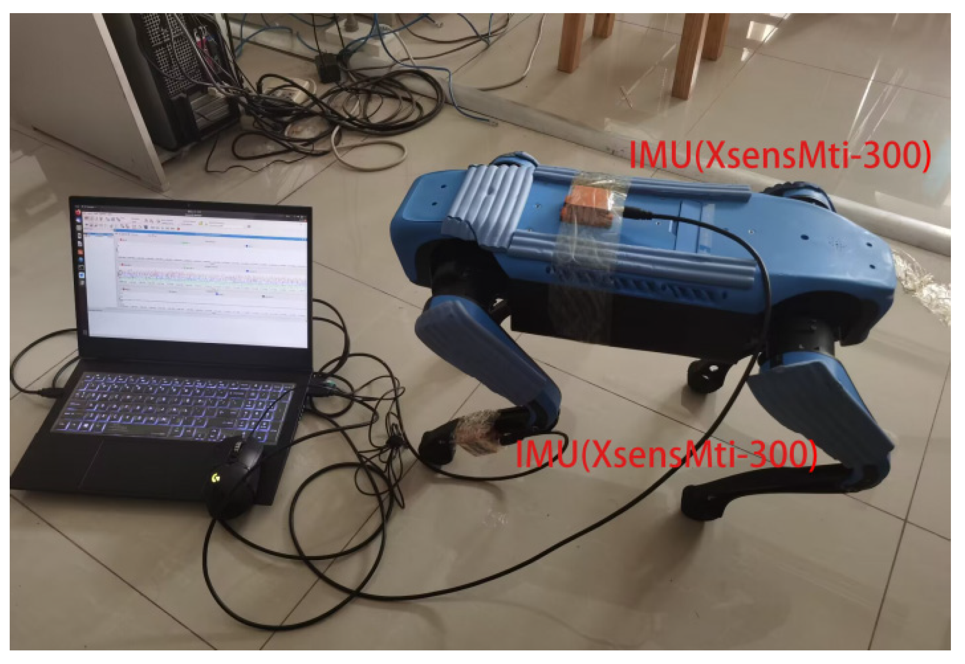
The data collection and construction of the virtual inertial sensor of the quadruped robot involve a deep learning computer and two distributed inertial sensors installed on the torso and feet of the quadruped robot, as shown in
Figure 2. The foot-mounted IMU should be located 1.97 inches away from the bottom of the foot, and the torso should be located in the center of the torso. These two distributed inertial sensors synchronously collect the motion inertial data of the quadruped robot. The deep learning network model classifies the inertial sensor information of the torso and constructs the virtual inertial sensor of the foot of the quadruped robot [
9].
3.2.1. Construction of Virtual Inertial Sensor Based on Deep Learning
In this study, we employed the squeeze-and-excitation network (SENet) as the attention-based CNN model for gait classification training. Compared with traditional CNN models [
10], SENet employs a weakly labeled dataset for model training [
11]. By learning the weights of each channel, it enhances the ability to identify various channel features and improves the accuracy of gait classification from torso’s inertial sensor data [
12]. The detailed working process and mathematical model algorithm of the SENet model are described in the literature [
13].
Figure 2.
Hardware installation of the quadruped robot’s virtual inertial sensor construction.
Figure 2.
Hardware installation of the quadruped robot’s virtual inertial sensor construction.
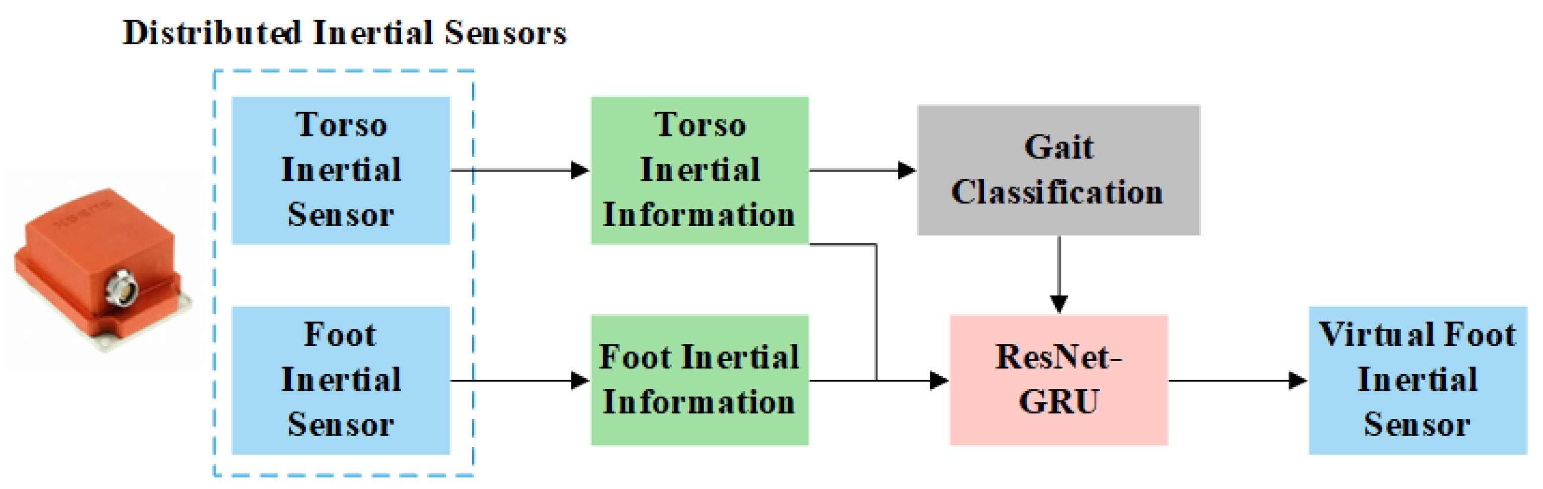
Through gait classification, we used a hybrid ResNet–GRU model to extract the nonlinear mapping relationship between the inertial sensor data of the torso and feet and to construct a virtual inertial sensor of the feet, The detailed flow is shown in
Figure 3. The model trains virtual inertial sensor models for each gait type, which reduces the difficulty of fitting the mapping relationship of the inertial sensor and improves the regression accuracy of the hybrid model.
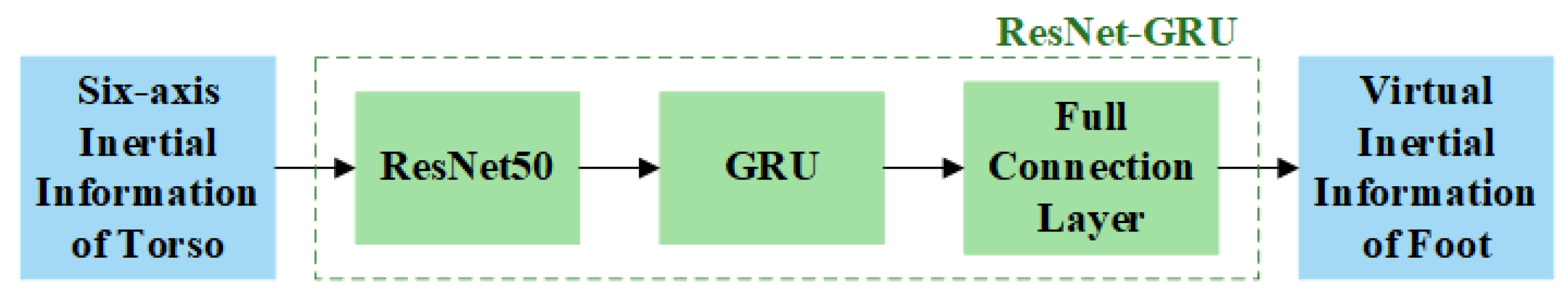
This is shown in
Figure 4, the hybrid ResNet–GRU model captures the local correlation features in the inertial sensor data using ResNet [
14,
15], learns and extracts the motion feature data hidden in the input data, and employs the GRU neural network to further extract the temporal features of the inertial data by receiving the feature fragments from ResNet [
16]. The features extracted by the model are all input into the fully connected layer to establish a nonlinear mapping relationship between the inertial sensor data of the torso and feet, constructing a virtual inertial sensor of the foot based on the hybrid ResNet–GRU model. The detailed structure of the hybrid ResNet–GRU model is described in the literature [
17].
3.2.2. Virtual Inertial Navigation System Based on Zero-velocity Update
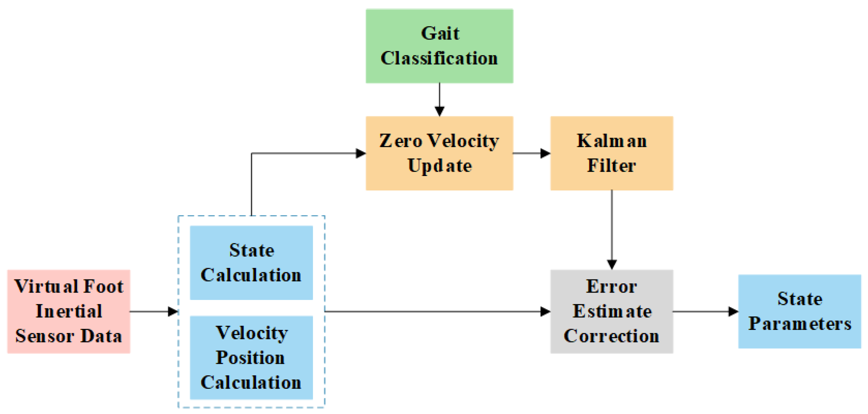
After the foot virtual inertial sensor is constructed, the VINS calculates and estimates the state parameters of the foot robot using the strapdown inertial navigation algorithm. To address the cumulative error of the inertial navigation system, the system uses the corrected state parameters via the zero-velocity detection algorithm to assist the system to complete the state estimation. The detailed flow is shown in
Figure 5. The flow of the strapdown inertial navigation and zero-velocity detection algorithm and related formulas are described in the literature [
18].
Due to the differences in the distribution of zero-velocity intervals across different motion modes of the quadruped robot, the accuracy of zero-velocity correction can be affected. To reduce the misjudgment rate of zero-velocity intervals and improve the accuracy of the correction algorithm, the system introduces gait classification constraints and adjusts filtering parameters based on the motion mode.
In the zero-velocity detection algorithm, angular velocity is filtered and partitioned into search units using a sliding window averaging method. When the system detects a zero-velocity state during motion, the Kalman filter is activated to estimate and correct output error. More details on the error mathematical model and the Kalman filter algorithm can be found in the literature [
19].
3.2.3. Virtual Inertial Navigation System Performance Verification
In this study, we first tested the accuracy of gait classification. It can be seen from
Table 1 that the attention-based CNN model could achieve a gait classification rate of approximately 97.6%. Considering that the hybrid ResNet–GRU model has the ability to tolerate faults, the gait classification accuracy achieved in the experiment was adequate for the further construction of virtual inertial sensors.
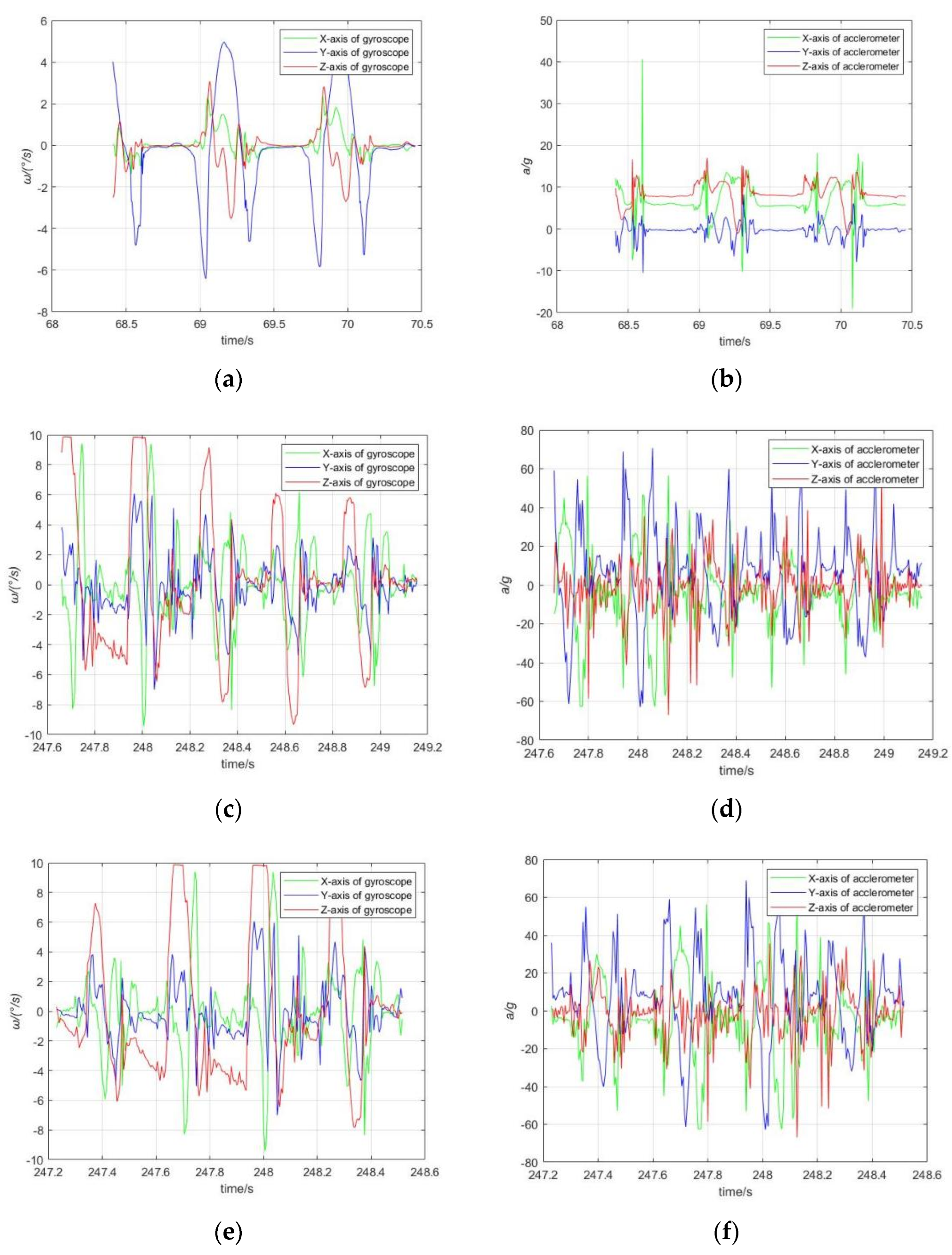
We also collected torso and foot inertial sensor data to validate three typical gaits of the quadruped robot: walking, running, and uphill/downhill walking.
Figure 6b,d and f show the acceleration output curves; and
Figure 6a,c and e show the gyroscope output curves of the virtual IMU for different walking motions of the quadruped robot. A comparison between the virtual inertial sensor data constructed using the hybrid ResNet–GRU network model and the actual foot inertial sensor data is shown in
Table 1.
The virtual inertial sensors constructed using the hybrid ResNet–GRU network model were compared with the actual foot inertial sensor data.
Figure 6 shows the fitting curves, and we do not present the actual collected curves as the errors between the two were too small to distinguish. During motion, the amplitude of motion information is much larger than the order of magnitude of the fitting error, making it difficult to identify the fitting error on the curve.
In the comparison results presented in
Table 2, it can be seen that the fitting curves of the virtual inertial sensor have a similar identification accuracy and a small curve error to the actual foot inertial sensor in the case of relatively intense movements such as the uphill and downhill movement of the quadruped robot. As in the previous study, the results meet the positioning accuracy requirements of the inertial navigation system.
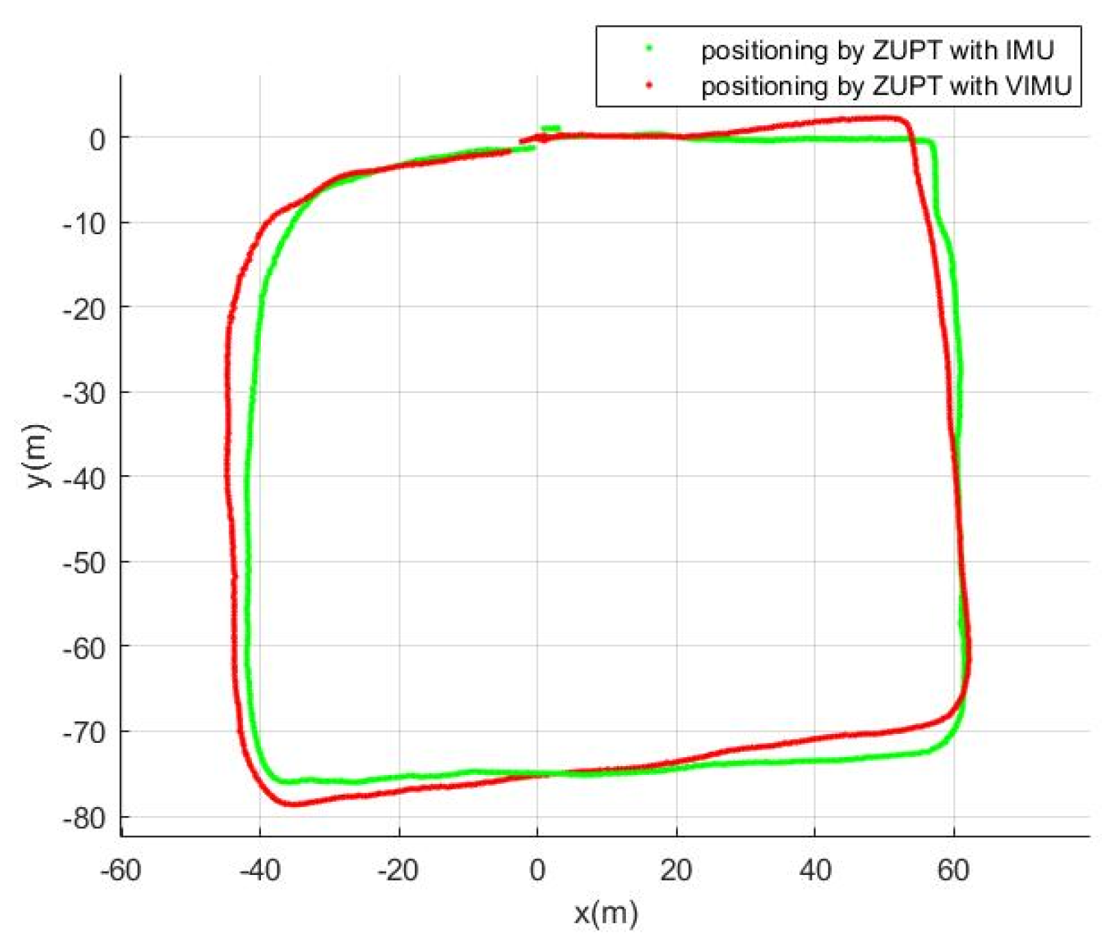
The experiment was conducted on a three-dimensional route with a total distance of about 350 m, involving gait types such as walking and traveling uphill and downhill. The red and green lines represent the output of IMU and VIMU, respectively. By comparison, the positioning error of the VIMU output was about 4.3% compared with that of the IMU. From the experimental results, it can be seen that the VIMU cannot completely replace the IMU. Therefore, the VIMU is only used to rebuild the inertial navigation system when it fails.
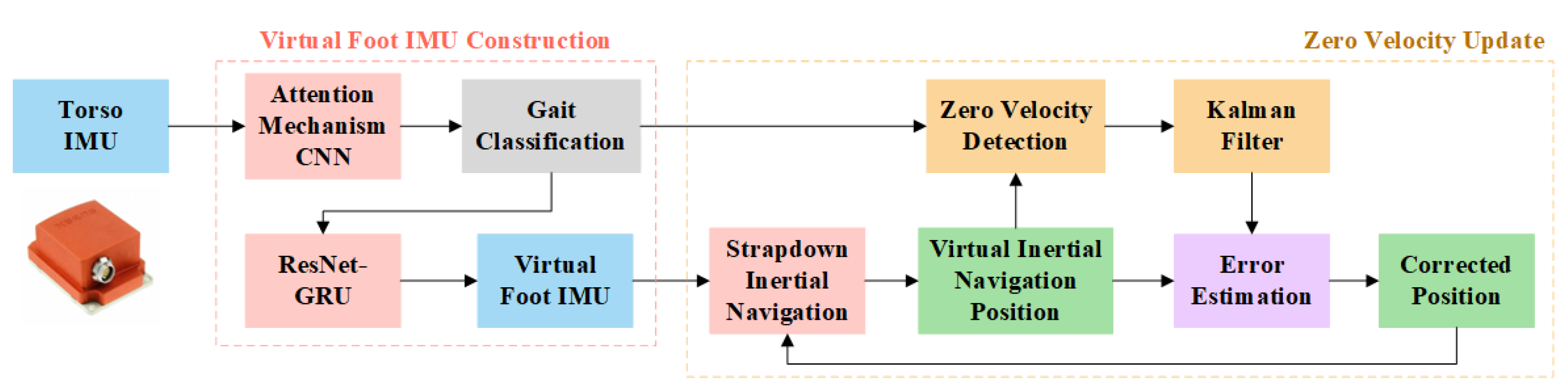
Based on the virtual inertial sensor outputs, the proposed system effectively ensured range integrity and showed strong adaptability in complex environments [
20]. The VINS employs a virtual inertial sensor constructed based on a deep learning network model. Through zero-velocity detection, it utilizes zero-velocity detection to estimate and correct the pose error outputted by the strapdown inertial navigation algorithm, and the corrected state parameters are used to assist the system in completing the pose estimation.
The corrected state parameters generated by the VINS are used to adjust the state parameters of the LiDAR’s inertial odometer. The corrected state parameters are then transmitted to the LIDAR mapping module to enhance the accuracy of global map construction, as shown in
Figure 7.
As shown in
Figure 8, we utilized the walking gait to navigate around a building and validate the positioning accuracy of the VIMU in comparison with that of the IMU system. Despite encountering potential external interference during the data acquisition process, the VIMU still satisfactorily fulfilled the system’s positioning accuracy requirements when compared with the positioning effect of IMU.
4. Analysis of LINS Performance in Degenerate Environments
This study analyzed the localization and mapping performance of a LiDAR–inertial fusion system in degenerate environments based on the LINS algorithm [
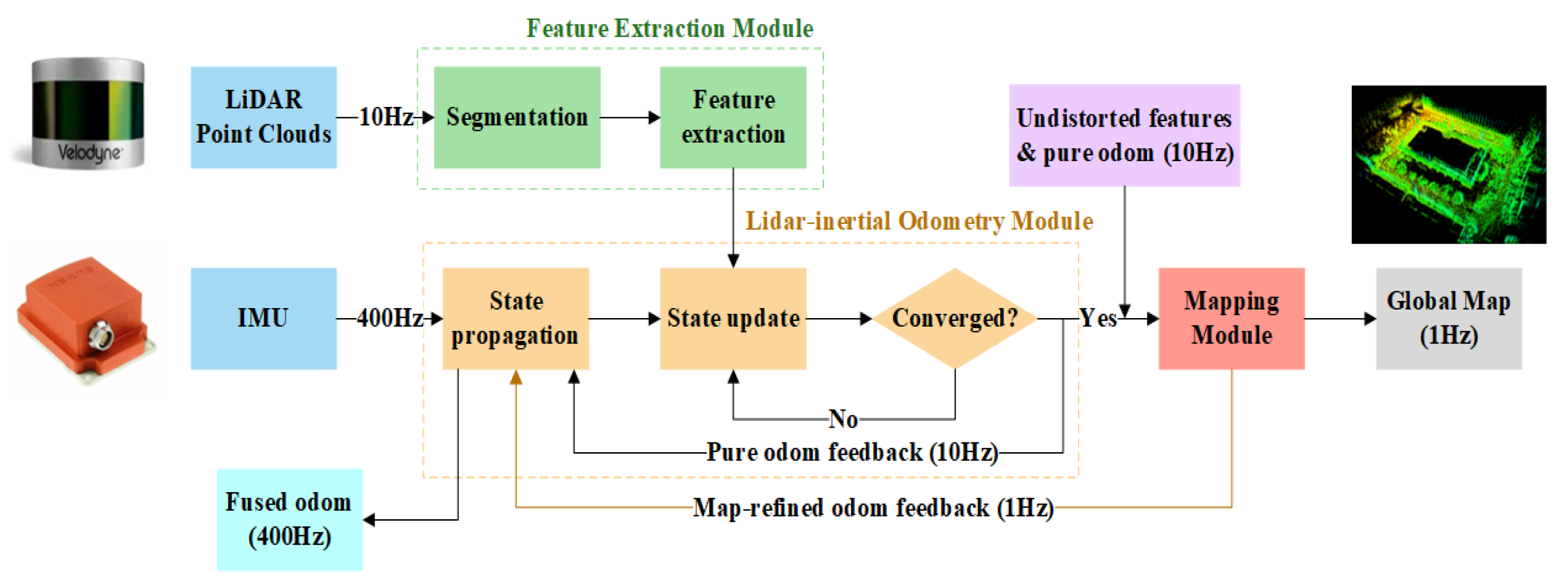
21]. LINS is a well-established LIDAR inertial fusion algorithm that estimates pose information and generates maps by fusing LiDAR point clouds with inertial sensor data. The detailed flowchart is shown in
Figure 9.
First, the LiDAR point clouds are segmented and feature points are extracted using the feature extraction module. To uniformly extract features from all directions, the range image is divided into several equal subimages, and different types of features are distinguished based on the curvature
c [
22].
where
represents the point cloud composed of point
as the center,
and
are the point in
. When the LiDAR–inertial navigation system is used for localization and mapping in degenerate environments, the calculated curvature
values are often small or even close to zero, resulting in fewer detected feature corner points in degenerate environments.
Next, the features extracted from the feature extraction module are inputted to the LIO module for pose estimation [
23]. The module utilizes the point cloud matching method to calculate the relative transformation relationship between LiDAR point cloud frames by computing the distance
d between corner points.
where
represents the position of the point on the current frame in the point cloud coordinate system of the previous frame;
and
represent the positions of each point in the previous frame’s point cloud.
Due to the limited number of feature corner points that can be extracted in degenerate environments by the feature extraction module, the distance between feature points is large, and the error in calculating the distance is significant. This leads to lower optimization performance in point cloud matching and larger cumulative error in the pose estimation of the LIO module, even for the points affecting the optimization of motion distortion in the point clouds.
Finally, the LiDAR mapping module builds a global map by integrating the pose information provided by the LIO module with the current frame of point clouds. However, due to the cumulative error in the pose estimation of the LIO module in degenerate environments and the decreased performance in optimizing the motion distortion of the point clouds, the global map constructed by the LiDAR mapping module may have significant errors.
Considering the significant localization and mapping errors of the LiDAR inertial navigation system in degenerate environments, this paper proposes a VINS-assisted localization method, which effectively improves the robustness of quadruped robot localization and mapping in degenerate environments.
4.1. Performance Verification Experiment of Sparse and Degenerate Scene of Unidirectional Structural Features
LINS and other LiDAR–inertial navigation systems have effectively improved the robustness of robot localization and mapping in complex environments by calculating fused state parameters. However, in some degenerate environments, such as featureless areas, significant errors may arise due to missing feature points in the LiDAR–inertial odometry. Based on the extent of degeneration areas, the system accumulates errors in the LiDAR–inertial odometry operation for longer durations.
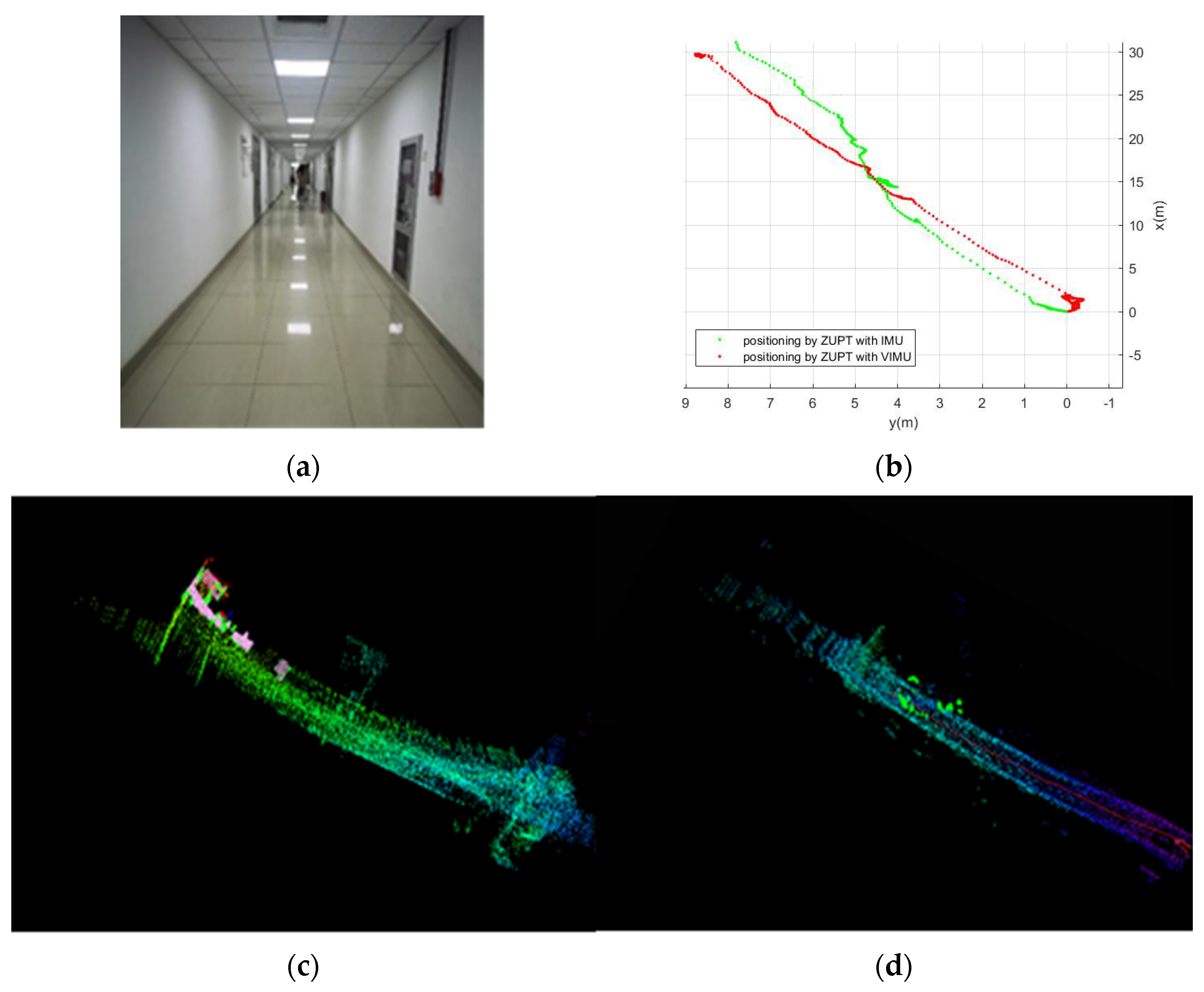
Experiment 1 was conducted in a degenerate environment consisting of a long straight corridor, as shown in
Figure 10a. The corridor exhibited a one degree of freedom direction (1DOF) degeneration characteristic along its axis. Additionally, the presence of interference from lighting and reflective ground led to significant LINS localization deviation. The quadruped robot equipped with a LiDAR and the inertial sensor started the experiment at the center of the starting segment, and we conducted localization and mapping experiments along its axis for the entire corridor. We used the floor tile joints as our movement route and reference points. The positioning and mapping of the LINS and VIMU with LINS for point clouds are shown in
Figure 10.
Based on the experimental results shown in
Figure 10b, the LINS method yielded gradually increasing offset errors in the sparse feature points of the corridor’s middle section, resulting in a significant discrepancy between the output localization trajectory and the actual path at the end of the corridor. The resulting point cloud map failed to accurately reflect the actual shape of the model. Furthermore, the positioning output results of the LINS method appeared stationary and moved in the opposite direction as the robot advanced along the corridor axis, leading to the accumulation of errors and eventual positioning failure in the corresponding LiDAR point clouds.
Figure 10 compares the performance between the proposed method and LINS. The former exhibited high accuracy in the middle section of the corridor without any point cloud overlap issue. Using the middle line of the corridor as the reference path, the relative errors between the two methods’ positioning trajectory output and the actual value could be computed. The relative error of LINS was 46%, while the relative error of the proposed method was 15%. Thus, in degenerate scenario 1, the positioning trajectory output and the point clouds map agreed well with the scene model.
4.2. Performance Verification Experiment of Sparse and Degenerate Scene of Multidirectional Structural Features
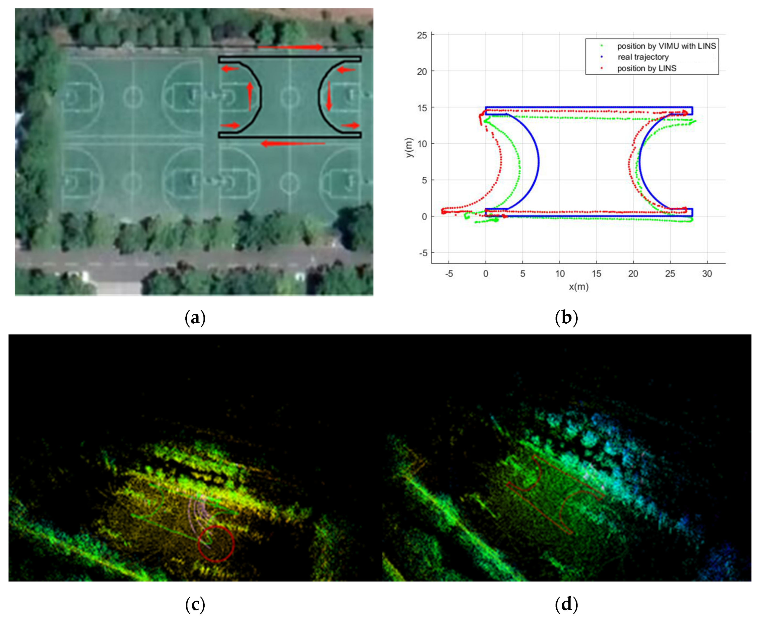
The degenerate environment in Experiment 2 was a standard basketball court in an open outdoor environment, as shown in
Figure 11a. The actual route was the real trajectory collected by GPS, which served as our route basis. The central area of the basketball court was an open space with sparse feature points, which resulted in a multidirectional degenerate scenario due to the lack of surrounding directional constraints. LiDAR–inertial navigation system can only use ground point clouds for matching. In this experiment, the quadruped robot was controlled to start walking from a rich-feature area at one end of the basketball court from a stationary position, following the standard court boundary, as shown in
Figure 11a. A comparison between LINS and the assisted navigation system with the VINS of the point clouds and localization is shown in
Figure 11b.
As shown in
Figure 11c,d, the trajectory at the start of the localization output from the LINS method without the degradation analysis process roughly matched the robot’s trajectory. Because of the sparse point cloud data in the central open area and the tendency of inertial sensors to exceed their range during sudden changes in motion, the LINS method experienced repeated point clouds and positioning errors at corners, resulting in a cumulative increase in error over time. As shown in
Figure 12a, the point cloud density of the assisted navigation system with the VINS was much higher, and there was no overlap of the point clouds at the corners due to repeated map building. The VINS system uses a virtual inertial sensor for positioning, making it more robust in dealing with over-range issues due to abrupt motion. As a result, it can maintain good positioning accuracy in sharp corners and achieve high accuracy in both positioning and map building in multidirectional degenerate environments.
4.3. Overall Performance Verification Experiments
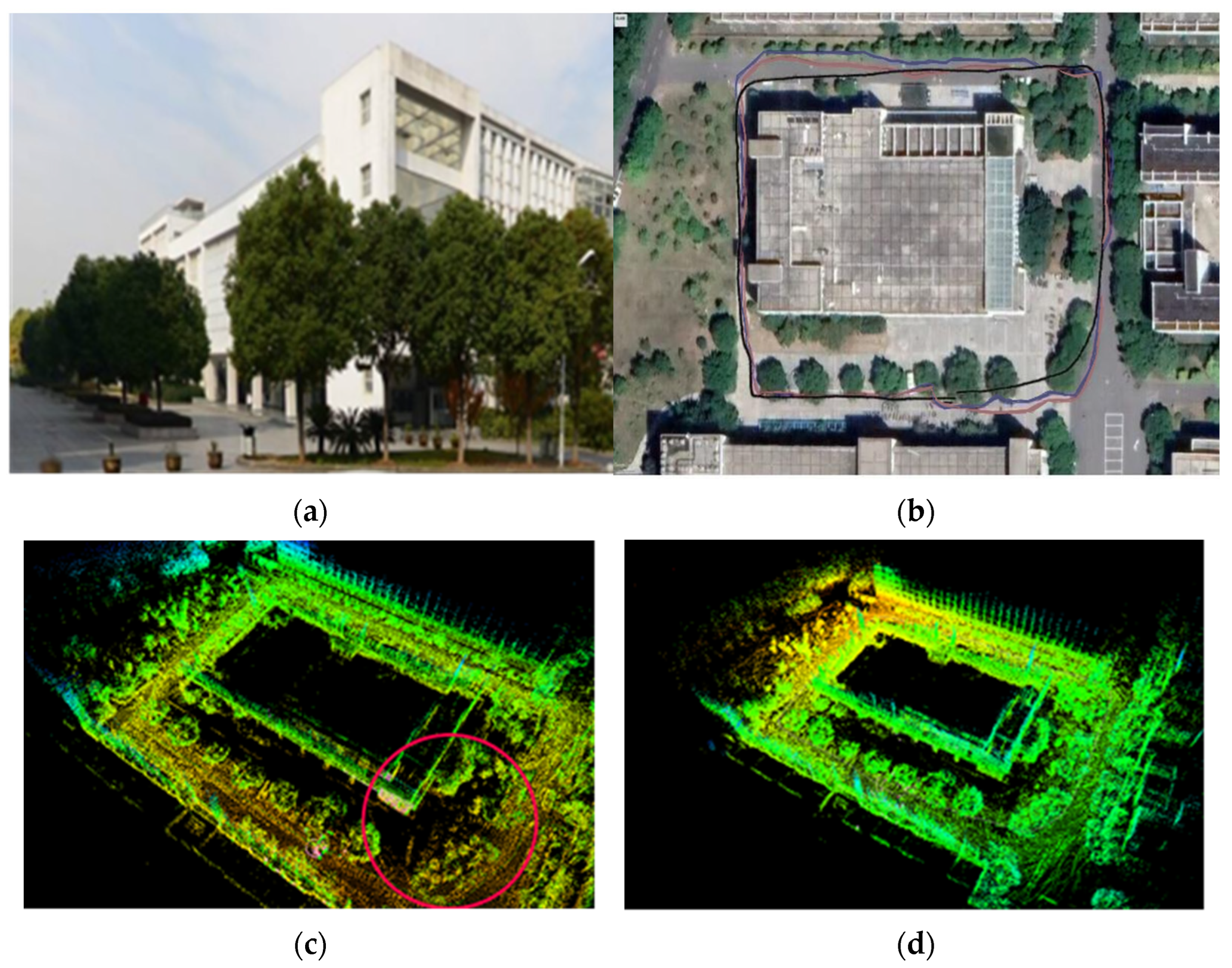
Experimental scenario 3 involved a building complex on campus. The actual scene of the building is shown in
Figure 12a. There were open areas in part of the scene, leading to environmental degeneration, and the quadruped robot walked around the building in a circle to test the performance of the LiDAR–inertial navigation system for positioning and mapping.
As shown in
Figure 12b, the black line is the DGPS reference trajectory, the blue line is the trajectory of the LINS method, and the red line is the trajectory of the assisted LINS with VIMU; compared with the LINS, the positioning effect of the VIMU with LINS is closer to the actual path and demonstrates stable and better performance at turning points. In the VINS-assisted LINS method, the average positioning error was 1.20 m, and the frame rate was 30 Hz, which meet the real-time positioning requirements of quadruped robots. At the same time, the LINS method was measured under the same conditions, and the average positioning error was 1.08 m, demonstrating the effectiveness of the assisted method. The point clouds maps of the LINS and VIMU with LINS are shown in
Figure 12c,d.
The point cloud map of LINS with VINS achieved an RMSE [
24] of 9.33/cm, and the LINS point cloud map has an RMSE of 11.6/cm. The LINS with VINS had a higher point cloud density, which could more accurately reflect the actual situation when in open areas. At the same time, the optimized point cloud map has clearer contours and less deformation at building corners; the problem of repeated scanning of the same object was also solved.
5. Conclusions
In this paper, we propose a VINS method to assist localization and mapping in degenerate environments. This method employs a deep learning network model to construct virtual inertial sensors and is coupled with a shortcut inertial navigation algorithm and a zero-velocity correction algorithm to assist the LiDAR–inertial navigation system in correcting the state parameters obtained from the LiDAR–inertial odometer, improving the accuracy of the SLAM process.
The experimental results indicate that the robustness of localization and mapping for quadruped robots in typical degenerate environments is greatly enhanced with the assistance of VINS and meets the localization accuracy requirements of quadruped robots. These findings suggest that VINS provides a promising support for the development of SLAM technology in degenerate environments.
Additionally, the broad applicability of the algorithm across both quadruped robots and wearable devices for humans underscores its versatility. This wider scope of potential applications extends beyond quadruped robots and encompasses domains such as autonomous driving, robot navigation, wearable devices, and other related fields. Consequently, the findings from this research suggest that VINS holds promise in advancing the development of simultaneous localization and mapping (SLAM) technology in degenerate environments.
Author Contributions
Conceptualization, Y.C., J.Z. and J.D.; Methodology, Y.C.; Software, Y.C.; Validation, Y.C., J.Z. and K.W.; Formal Analysis, J.D.; Investigation, K.W.; Resources, Y.C.; Data Curation, J.Z.; Writing—Original Draft Preparation, Y.C. and J.Z.; Writing—Review and Editing, J.D. and T.S.; Visualization, Y.C.; Supervision, W.Q.; Project Administration, W.Q. All authors have read and agreed to the published version of the manuscript.
Funding
This research received no external funding.
Data Availability Statement
Not applicable.
Conflicts of Interest
The authors declare no conflict of interest.
References
- Cadena, C.; Carlone, L.; Carrillo, H.; Latif, Y.; Scaramuzza, D.; Neira, J.; Reid, I.; Leonard, J.J. Past, Present, and Future of Simultaneous Localization and Mapping: Toward the Robust-Perception Age. IEEE Trans. Robot. 2016, 32, 1309–1332. [Google Scholar] [CrossRef] [Green Version]
- Ji, Z.; Singh, S. Low-drift and Real-time LIDAR Odometry and Mapping. Auton. Robot. 2017, 41, 401–416. [Google Scholar]
- Zhao, S.; Fang, Z.; Li, H.; Scherer, S. A Robust Laser-Inertial Odometry and Mapping Method for Large-Scale Highway Environments. In Proceedings of the 2019 IEEE/RSJ International Conference on Intelligent Robots and Systems (IROS), Macau, China, 3–8 November 2019. [Google Scholar]
- Koizumi, M.; Nonaka, K.; Sekiguchi, K. Avoidance of singular localization environment using model predictive control for mobile robots. In Proceedings of the 2017 11th Asian Control Conference (ASCC), Gold Coast, QLD, Australia, 17–20 December 2017; pp. 2866–2871. [Google Scholar] [CrossRef]
- Zhang, J.; Kaess, M.; Singh, S. On degeneracy of optimization-based state estimation problems. In Proceedings of the 2016 IEEE International Conference on Robotics and Automation (ICRA), Stockholm, Sweden, 16–21 May 2016; pp. 809–816. [Google Scholar]
- Shao, W.; Vijayarangan, S.; Li, C.; Kantor, G. Stereo Visual Inertial LIDAR Simultaneous Localization and Mapping. In Proceedings of the 2019 IEEE/RSJ International Conference on Intelligent Robots and Systems (IROS), Macau, China, 3–8 November 2019; pp. 370–377. [Google Scholar] [CrossRef] [Green Version]
- Zhen, W.; Scherer, S. Estimating the Localizability in Tunnel-like Environments using LIDAR and UWB. In Proceedings of the 2019 International Conference on Robotics and Automation (ICRA), Montreal, QC, Canada, 20–24 May 2019; pp. 4903–4908. [Google Scholar] [CrossRef]
- Zhen, W.; Zeng, S.; Soberer, S. Robust localization and localizability estimation with a rotating laser scanner. In Proceedings of the IEEE International Conference on Robotics and Automation, Singapore, 29 May–3 June 2017; pp. 6240–6245. [Google Scholar] [CrossRef]
- Qian, W.; Zhu, Y.; Jin, Y.; Yang, J.; Qi, P.; Wang, Y.; Ma, Y.; Ji, H. A Pedestrian Navigation Method Based on Construction of Adapted Virtual Inertial Measurement Unit Assisted by Gait Type Classification. IEEE Sens. J. 2021, 21, 15258–15268. [Google Scholar] [CrossRef]
- Jetley, S.; Lord, N.A.; Lee, N.; Torr, P.H.S. Learn to Pay Attention. arXiv 2018, arXiv:1804.02391. [Google Scholar] [CrossRef]
- Xu, X.; Li, W.; Xu, D.; Tsang, I.W. Co-Labeling for Multi-View Weakly Labeled Learning. IEEE Trans. Pattern. Anal. Mach. Intell. 2016, 38, 1113–1125. [Google Scholar] [CrossRef] [PubMed]
- Wang, L.; Zang, J.; Zhang, Q.; Niu, Z.; Hua, G.; Zheng, N. Action recognition by an attention-aware temporal weighted convolutional neural network. Sensors 2018, 18, 1979. [Google Scholar] [CrossRef] [PubMed] [Green Version]
- Hu, J.; Shen, L.; Sun, G. Squeeze-and-Excitation Networks. Available online: http://image-net.org/challenges/LSVRC/2017/results (accessed on 1 January 2023).
- He, K.; Zhang, X.; Ren, S.; Sun, J. Deep residual learning for image recognition. In Proceedings of the IEEE Computer Society Conference on Computer Vision and Pattern Recognition, Las Vegas, NV, USA, 27–30 June 2016; pp. 770–778. [Google Scholar] [CrossRef] [Green Version]
- He, K.; Zhang, X.; Ren, S.; Sun, J. Identity Mappings in Deep Residual Networks. arXiv 2016, arXiv:1603.05027. [Google Scholar] [CrossRef]
- Cho, K.; van Merrienboer, B.; Bahdanau, D.; Bengio, Y. On the Properties of Neural Machine Translation: Encoder-Decoder Approaches. arXiv 2014, arXiv:1409.1259. [Google Scholar] [CrossRef]
- Xiao, X.; Li, K. Multi-Label Classification for Power Quality Disturbances by Integrated Deep Learning. IEEE Access 2021, 9, 152250–152260. [Google Scholar] [CrossRef]
- Fan, Q.; Sun, Y.; Sun, B.; Zhuang, X. Pedestrian Indoor Positioning System Based on GLRT Zero Speed Detection. Chin. J. Sens. Actuators 2017, 30, 1706–1711. [Google Scholar]
- Liu, J.Y. Theory and Application of Navigation System; Northwestern Polytechnical University Press: Xi’an, China, 2010. [Google Scholar]
- Qin, C.; Ye, H.; Pranata, C.E.; Han, J.; Zhang, S.; Liu, M. LINS: A Lidar-inertial State Estimator for Robust and Efficient Navigation. arXiv 2019, arXiv:1907.02233. [Google Scholar] [CrossRef]
- Zhang, J.; Singh, S. LOAM: LIDAR Odometry and Mapping in Real-time. In Robotics: Science and Systems; Carnegie Mellon University: Pittsburgh, PA, USA, 2014; Volume 2. [Google Scholar] [CrossRef]
- Shan, T.; Englot, B. LeGO-LOAM: Lightweight and Ground-OptimizedLIDAR Odometry and Mapping on Variable Terrain. In Proceedings of the 2018 IEEE/RSJ International Conference on Intelligent Robots and Systems (IROS), Madrid, Spain, 1–5 October 2018; IEEE: Piscataway, NJ, USA, 2018. [Google Scholar]
- Shan, T.; Englot, B.; Meyers, D.; Wang, W.; Ratti, C.; Rus, D. LIO-SAM: Tightly-coupled LIDAR Inertial Odometry via Smoothing and Mapping. arXiv 2020, arXiv:2007.00258. [Google Scholar] [CrossRef]
- Zhang, Z.; Scaramuzza, D. A Tutorial on Quantitative Trajectory Evaluation for Visual(-Inertial) Odometry. In Proceedings of the 2018 IEEE/RSJ International Conference on Intelligent Robots and Systems (IROS), Madrid, Spain, 1–5 October 2018; IEEE: Piscataway, NJ, USA, 2019. [Google Scholar]
Figure 1.
Detailed flowchart of implementation.
Figure 1.
Detailed flowchart of implementation.
Figure 3.
Flowchart of virtual inertial sensor construction.
Figure 3.
Flowchart of virtual inertial sensor construction.
Figure 4.
Flowchart of ResNet–GRU hybrid model structure.
Figure 4.
Flowchart of ResNet–GRU hybrid model structure.
Figure 5.
Flowchart of zero-velocity update process of virtual inertial navigation system.
Figure 5.
Flowchart of zero-velocity update process of virtual inertial navigation system.
Figure 6.
Virtual inertial sensor outputs of the quadruped robot during different gaits using the virtual IMU constructed in this study. (a) The virtual IMU’s gyroscope outputs during uphill and downhill motion. (b) The virtual IMU’s accelerometer outputs during uphill and downhill motion. (c) The virtual IMU’s gyroscope outputs during walking motion. (d) The virtual IMU’s accelerometer outputs during walking motion. (e) The virtual IMU’s gyroscope outputs during running motion. (f) The virtual IMU’s accelerometer outputs during running motion.
Figure 7.
Flowchart of the virtual inertial navigation system.
Figure 7.
Flowchart of the virtual inertial navigation system.
Figure 8.
Verification of positioning accuracy of virtual inertial navigation system.
Figure 8.
Verification of positioning accuracy of virtual inertial navigation system.
Figure 9.
Flowchart of LINS SLAM.
Figure 9.
Flowchart of LINS SLAM.
Figure 10.
(a) Actual scene of the straight corridor. (b) Comparison of positioning results between LINS and VIMU with LINS. (c) Mapping results of LINS. (d) Mapping results of VIMU with LINS.
Figure 10.
(a) Actual scene of the straight corridor. (b) Comparison of positioning results between LINS and VIMU with LINS. (c) Mapping results of LINS. (d) Mapping results of VIMU with LINS.
Figure 11.
(a) Actual scene and trajectory. (b) Comparison of LINS, VIMU with LINS, and actual trajectory. The actual route refers to the real trajectory collected by GPS, which served as the basis. (c) Point clouds map by LINS. (d) Point clouds map by VIMU with LINS.
Figure 11.
(a) Actual scene and trajectory. (b) Comparison of LINS, VIMU with LINS, and actual trajectory. The actual route refers to the real trajectory collected by GPS, which served as the basis. (c) Point clouds map by LINS. (d) Point clouds map by VIMU with LINS.
Figure 12.
(a) Actual campus building scene. (b) Positioning results of differential GPS, LINS, and VIMU with LINS. (c) Point cloud maps of LINS. (d) Point cloud maps of VIMU with LINS.
Figure 12.
(a) Actual campus building scene. (b) Positioning results of differential GPS, LINS, and VIMU with LINS. (c) Point cloud maps of LINS. (d) Point cloud maps of VIMU with LINS.
Table 1.
Classification accuracy of attention-based CNN model gait types.
Table 1.
Classification accuracy of attention-based CNN model gait types.
| | Walking | Running | Uphill | Downhill |
|---|
| Walking | 343 | 2 | 2 | 1 |
| Running | 4 | 341 | 1 | 1 |
| Uphill | 1 | 3 | 340 | 1 |
| Downhill | 2 | 1 | 1 | 342 |
Table 2.
Virtual inertial sensor output fitting error, where a and w, respectively, represent accelerometers and gyroscopes; M is the output deviation of the IMU; and S is the output noise of the IMU.
Table 2.
Virtual inertial sensor output fitting error, where a and w, respectively, represent accelerometers and gyroscopes; M is the output deviation of the IMU; and S is the output noise of the IMU.
| | Mw (°/s) | Sw (°/s) | Ma (m/s2) | Sa (m/s2) |
|---|
| Walking | 0.0009 | 0.0010 | 0.046 | 0.088 |
| Running | 0.0021 | 0.0037 | 0.072 | 0.121 |
| Uphill | 0.0011 | 0.0019 | 0.050 | 0.092 |
| Downhill | 0.0014 | 0.0020 | 0.058 | 0.098 |
| Disclaimer/Publisher’s Note: The statements, opinions and data contained in all publications are solely those of the individual author(s) and contributor(s) and not of MDPI and/or the editor(s). MDPI and/or the editor(s) disclaim responsibility for any injury to people or property resulting from any ideas, methods, instructions or products referred to in the content. |
© 2023 by the authors. Licensee MDPI, Basel, Switzerland. This article is an open access article distributed under the terms and conditions of the Creative Commons Attribution (CC BY) license (https://creativecommons.org/licenses/by/4.0/).


