Bifocal Dual Reflectarray with Curved Main Surface

Abstract

This paper presents a novel approach to synthesizing curved reflectarrays using Geometrical Optics (GO). It introduces the concepts of virtual normal and path length shift, which enable a vector-based formulation of the problem that can be solved using ray tracing techniques. The formulation is applied for the design of two different versions of a Dual Bifocal Reflectarray with a parabolic main surface and a flat subreflectarray. The first version aims to enhance the performance of the multibeam antenna by providing a focal ring located at the feed cluster plane. The second version focuses on improving the scanning characteristics of the antenna in the horizontal plane by incorporating two foci. The synthesis procedure yields samples of the path length shift or its derivatives. To reconstruct the phase distribution, an interpolation scheme is employed and described in this paper. Numerical results are presented for both the focal-ring and two-foci configurations, demonstrating the feasibility of this solution for multibeam or scanning satellite antennas operating in the Ka.

1. Introduction

Multibeam antennas for emerging communications satellites require an increasing number of spot beams that exploit different polarizations and frequencies [1]. The gain and beamwidth requirements of individual spots make it necessary to use of reflector or reflectarray systems fed by an appropriate cluster of feeding elements providing a color map of beams defined to achieve global coverage through frequency and polarization reuse. In a single-feed-per-beam (SFPB) configuration, due to the closely spaced beams required and the size limitation of the usable focal plane, traditional reflector antennas can provide only one color, and typically four reflector antennas are required, each operating in transmission (Tx) and reception (Rx). The field of view of these antennas, which is related to the scanning performance of the reflector or reflectarray systems, is one of the most critical factors in the design, due to the extensive use of the focal plane and the large coverage area compared to the size of a single beam.

It is known that bifocal dual reflector antennas [2,3,4] can improve the field of view of scanning antennas compared to the corresponding dual reflector versions with a single focus. The use of a dual reflector system introduces an additional degree of freedom, which can be utilized to ensure two privileged directions in the far field (or two focal targets in imaging applications) instead of requiring the condition that the main reflector and subreflector share a common focal point.

Reflectarray configurations have shown promise as solutions for multibeam antennas due to their ability to generate multiple beams using a single feed by polarization/frequency discrimination [5], or acting as a polarizer providing dual circular polarizations when illuminated by a signal in dual linear polarization [6].

The bifocal technique has been applied in dual reflectarray configurations [7,8,9] based on flat surfaces. In [7], a small size centered dual reflectarray antenna was proposed to improve the field of view in automotive radars operating in linear polarization. In [8], a procedure to compute the phase distribution of a bifocal dual reflectarray is presented for centered and offset configurations. In [9], a new bifocal design procedure for dual reflectarray antennas in offset configurations is presented. This procedure involves initially considering an axially symmetric geometry with the reflectarrays placed in parallel planes, and then tilting the reflectarray planes while readjusting the phases to avoid blockage effects.

For large aperture antennas, required for high gain multibeam antennas, using flat surface reflectarrays has the drawback of requiring a large phase adjustment with a high number of 2π cycles. This adjustment is necessary to transform the spherical waves provided by the feeds into a large aperture with an almost uniform phase, which is crucial for providing narrow beams in high frequency bands such as the Ka-band commonly used for satellite communications. A promising technique is to combine the focusing advantages of curved reflector surfaces such as the paraboloid with the control of reflection properties available with reflectarray solutions. An example of this combination was proposed in [6] to design a polarizing reflector that transforms linear polarization into dual polarization.

The shaping techniques based on Geometrical Optics (GO), typically used for reflector antennas, such as the bifocal technique, can be generalized to reflectarray surfaces by using the modified Snell Law, when phase control is added to the surface. This paper presents a novel formulation that considers GO shaping techniques in curved reflectarrays. It is based on the concept of path length shift, which is proportional to the phase adjustment in reflectarray surfaces, and the concept of virtual normal, which allows for a vector formulation for GO shaping and analysis of curved reflectarrays. The technique is illustrated throug the design of a bifocal dual reflectarray with flat subreflector and parabolic main reflectarray.

Section 2 and Appendix A present the treatment of the reflection equations for curved reflectarrays introducing the concepts of path length shift (proportional to the phase distribution) and the virtual normal (representing the reflection law at the reflectarray surface). Section 3 and Appendix B summarize the main characteristics of reflectarray analysis and synthesis for curved reflectarrays, as well as some interpolation algorithms for the treatment of the synthesized path length shift distributions that characterize the reflectarrays.

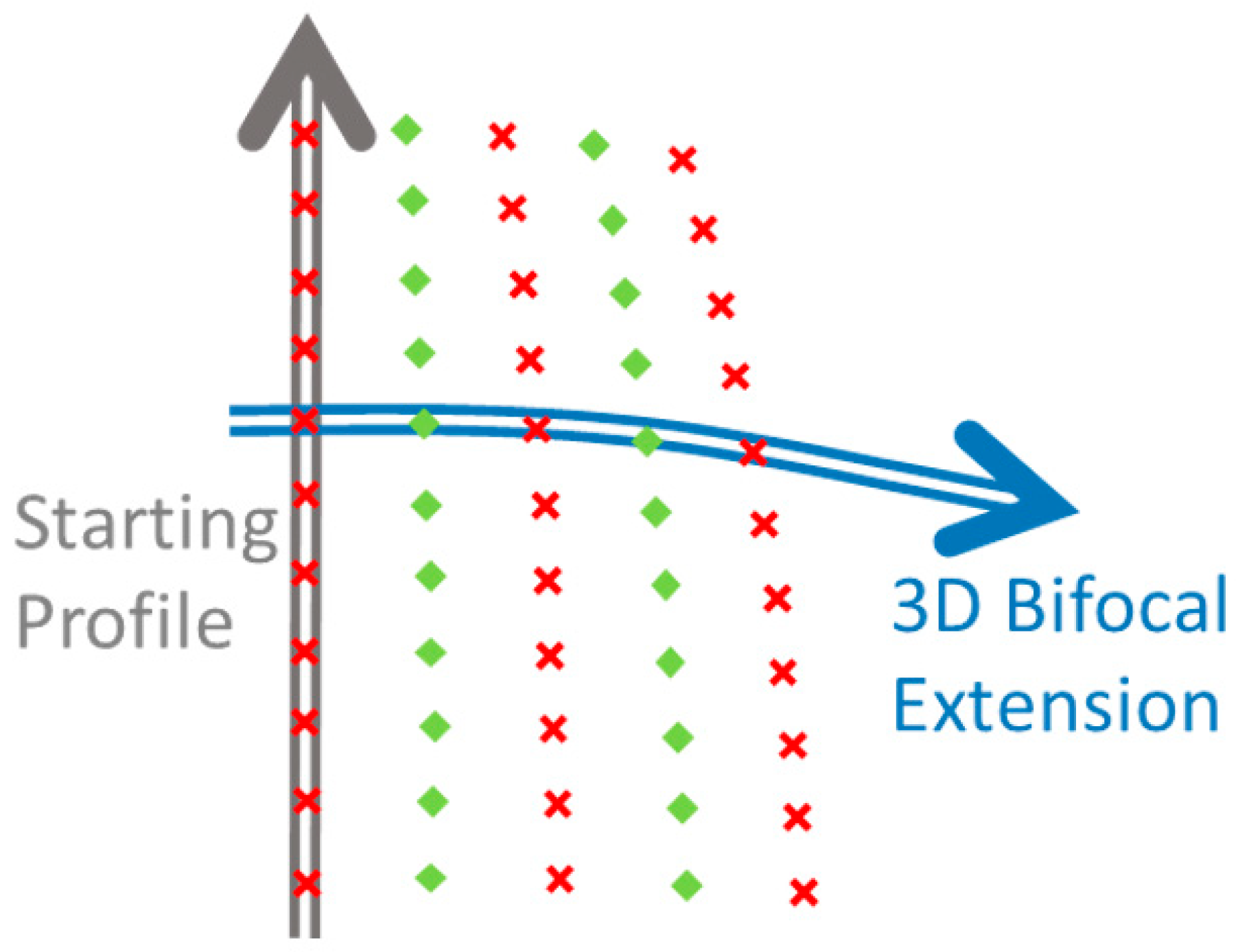
Section 4 presents the vector formulation of the bifocal synthesis algorithm applied to a curved reflectarray as the main surface fed from a flat sub-reflectarray. The synthesis of a line of data points is first formulated, followed by two examples of the 3D extension. Section 5 presents preliminary simulations of two different examples of bifocal reflectarrays defined for a multibeam satellite antenna in the Ka band. Finally, Section 6 presents the conclusions.

2. Reflection Equations for Curved Reflectarrays

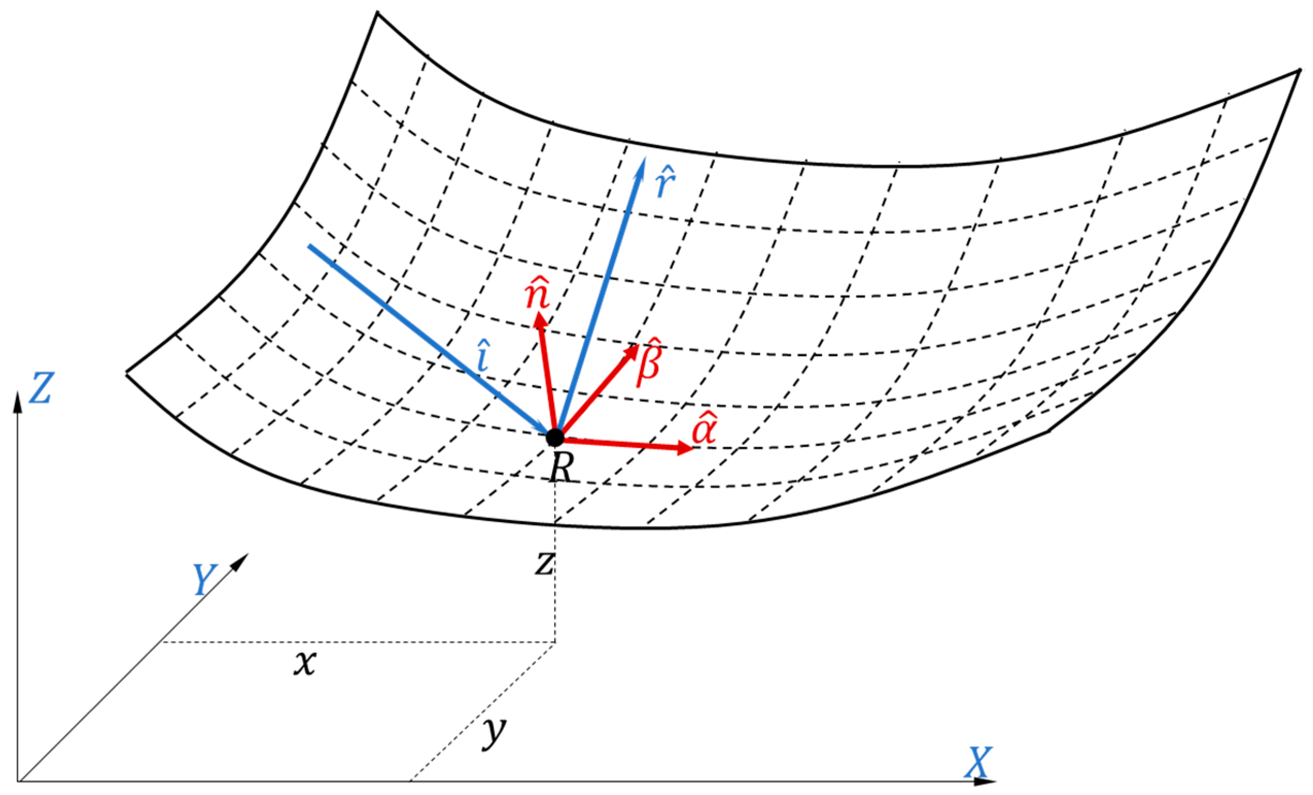
Figure 1 represents a reflectarray surface described in Cartesian coordinates by the function $z(x,y)$. The partial derivatives of the function with respect x and y are denoted as $z_x\left(x,y\right),z_y\left(x,y\right)$, respectively. All of them are known “a priori”, as well as the unit normal vector to the surface, denoted as $\widehat{n}$, which can be expressed as:

$$\widehat{n}=\frac{-z_x\widehat{x}-z_y\widehat{y}+\widehat{z}}{\sqrt{1+z_x^2+z_y^2}}.$$

(1)

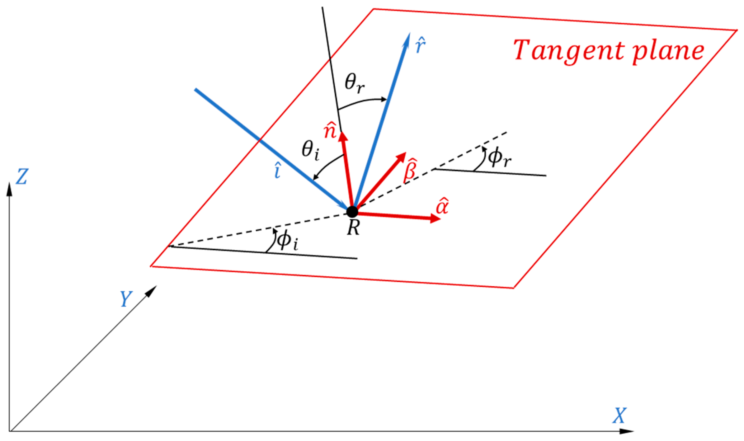
The figure also depicts a generic reflection point $R$, along with the incident ray ($\widehat{i}$) and reflected ray ($\widehat{r}$). Figure 2 provides a detailed view of the reflection point and a local reference system composed of the orthonormal vectors $\left\{\widehat{\alpha },\widehat{\beta },\widehat{n}\right\}$, where $\widehat{\alpha }$ and $\widehat{\beta }$ lie in the tangent plane to the surface at R.

For a reflectarray surface, a phase distribution denoted by $\Phi (x,y)$ can be defined at each point of the surface, representing the phase control introduced by the local reflectarray elements. Let $L\left(x,y\right)$ be the so-called path length shift, which is proportional to the phase shift introduced by the reflectarray elements at any point of the surface:

$$\Phi \left(x,y\right)=-kL\left(x,y\right)=-\frac{2\pi }{\lambda }L\left(x,y\right),$$

(2)

where $k$ is the propagation constant.

The unit vectors corresponding to the incident and reflected rays can be expressed in the system shown in Figure 2 as:

$$\begin{gathered} \widehat{r}=\mathit{sin}{\theta }_r\mathit{cos}{\varphi }_r\widehat{\alpha }+\mathit{sin}{\theta }_r\mathit{sin}{\varphi }_r\widehat{\beta }+\mathit{cos}{\theta }_r\widehat{n}, \\ \widehat{i}=\mathit{sin}{\theta }_i\mathit{cos}{\varphi }_i\widehat{\alpha }+\mathit{sin}{\theta }_i\mathit{sin}{\varphi }_i\widehat{\beta }-\mathit{cos}{\theta }_i\widehat{n}. \end{gathered}$$

(3)

According to [10], the tangential components of $\widehat{i}$ and $\widehat{r}$ are related to the partial derivatives of the phase shift across the surface:

$$\begin{gathered} \mathit{sin}{\theta }_r\mathit{cos}{\varphi }_r+\mathit{sin}{\theta }_i\mathit{cos}{\varphi }_i=-\frac{1}{k}\frac{\partial \Phi }{\partial \alpha }=\frac{\partial L}{\partial \alpha }, \\ \mathit{sin}{\theta }_r\mathit{sin}{\varphi }_r+\mathit{sin}{\theta }_i\mathit{sin}{\varphi }_i=-\frac{1}{k}\frac{\partial \Phi }{\partial \beta }=\frac{\partial L}{\partial \beta }. \end{gathered}$$

(4)

The virtual normal is then defined at $R$ as:

$$\overrightarrow{N}=\widehat{r}-\widehat{i}.$$

(5)

The main property of the virtual normal is that its tangential component ${\overrightarrow{N}}_{\tau }$ is not dependent on the incidence angle of the ray $\widehat{i}$, but it is directly related to the partial derivatives of $\Phi$ along the two tangential variables $\alpha ,\beta$, locally defined for the reflectarray surface around the reflection point $R$. The tangential vector ${\overrightarrow{N}}_{\tau }$ can be represented both in the Cartesian system and in the local tangential system composed of $\widehat{\alpha }$ and $\widehat{\beta }$:

$$\begin{gathered} {\overrightarrow{N}}_{\tau }=N_x\widehat{x}+N_y\widehat{y}+N_z\widehat{z}=N_{\alpha }\widehat{\alpha }+N_{\beta }\widehat{\beta }, \\ {N}_{\alpha }=\frac{\partial L}{\partial \alpha },N_{\beta }=\frac{\partial L}{\partial \beta }. \end{gathered}$$

(6)

Ray tracing techniques, which can be used to analyze a reflectarray, usually represent the rays in the absolute system $\left\{\widehat{x},\widehat{y},\widehat{z}\right\}$. For planar reflectarrays, it is possible to define a local orthonormal system $\left\{\widehat{\alpha },\widehat{\beta },\widehat{n}\right\}$ at the center of the reflectarray, and the transformation between local coordinates and absolute coordinates in the system $\left\{\widehat{x},\widehat{y},\widehat{z}\right\}$ is simple and allows for connecting ray tracing in the absolute system to the reflectarray characterization through the path length shift distribution $L\left(\alpha ,\beta \right)$ in the local system $\left\{\widehat{\alpha },\widehat{\beta },\widehat{n}\right\}$.

However, for curved reflectarrays, since the local system $\left\{\widehat{\alpha },\widehat{\beta },\widehat{n}\right\}$ varies across the surface, it is preferable to characterize the path length shift in the aperture domain through the function $L\left(x,y\right)$, where XY represents the aperture plane. As a result, it is necessary to relate the partial derivatives in the absolute system to the Cartesian components of ${\overrightarrow{N}}_{\tau }$. After some mathematical manipulations based on differential geometry (justified in detail in Appendix A), the following relation can be derived:

$$\left[\begin{array}{c}\frac{\partial L}{\partial x}\\ \frac{\partial L}{\partial y}\end{array}\right]=\left[\begin{array}{ccc}1& 0& z_x\\ 0& 1& z_y\end{array}\right]\left[\begin{array}{c}{N}_x\\ N_y\\ N_z\end{array}\right].$$

(7)

For the synthesis problem of the reflectarray, it is necessary to express $L(x,y)$ after determining ${\overrightarrow{N}}_{\tau }$ using ray tracing techniques. This can be achieved by obtaining the partial derivatives using (7) and then integrating the derivatives or employing an interpolation scheme, as described in Appendix B.

For the analysis problem of the synthesized reflectarray by means of ray tracing techniques, the inverse relation required to order to evaluate the Cartesian components of ${\overrightarrow{N}}_{\tau }$ in terms of the derivatives of $L$ with respect to the aperture coordinates ($x,y$). The following relation can also be derived by inverting (7), as described in Appendix A.

$$\left[\begin{array}{c}{N}_x\\ N_y\\ N_z\end{array}\right]=\frac{1}{1+z_x^2+z_y^2}\left[\begin{array}{cc}1+z_y^2& -z_x{z}_y\\ -z_x{z}_y& 1+z_x^2\\ z_x& z_y\end{array}\right]\left[\begin{array}{c}\frac{\partial L}{\partial x}\\ \frac{\partial L}{\partial y}\end{array}\right].$$

(8)

3. Geometrical Optics Analysis and Synthesis of Curved Reflectarrays

3.1. Analysis Problem: Ray Tracing Algorithm to Obtain the Reflected or Incident Ray

The ray tracing technique can be utilized to calculate a reflected ray at the reflectarray surface when the incident ray is known and the function $L(x,y)$ is characterized, as well as its partial derivatives $\partial L/\partial x$ and $\partial L/\partial y$. First, the intersection point $R$ between the incident ray $\widehat{i}$ and the reflectarray surface $z(x,y)$ is computed using geometric considerations, as well of the corresponding unit normal vector $\widehat{n}$. Once the $(x,y)$ coordinates of the reflection point are known, (8) allows us to obtain the tangential part ${\overrightarrow{N}}_{\tau }$ of the virtual normal. The tangential part of the vector $\widehat{r}$ can be calculated by inverting (5), considering only the tangential components. Then, the reflected direction $\widehat{r}$ can be reconstructed by adding the normal component, ensuring that it remains a unit vector:

$${\overrightarrow{i}}_{\tau }=\widehat{i}-\left(\widehat{i}·\widehat{n}\right)\widehat{n}, {\overrightarrow{r}}_{\tau }={\overrightarrow{i}}_{\tau }+{\overrightarrow{N}}_{\tau }, \widehat{r}={\overrightarrow{r}}_{\tau }+\widehat{n}\sqrt{1-{\left|{\overrightarrow{r}}_{\tau }\right|}^2}.$$

(9)

If the incident vector must be determined from the reflected one, a similar procedure can be used, but considering the following equations:

$${\overrightarrow{r}}_{\tau }=\widehat{r}-\left(\widehat{r}·\widehat{n}\right)\widehat{n}, {\overrightarrow{i}}_{\tau }={\overrightarrow{r}}_{\tau }-{\overrightarrow{N}}_{\tau }, \widehat{i}={\overrightarrow{i}}_{\tau }-\widehat{n}\sqrt{1-{\left|{\overrightarrow{i}}_{\tau }\right|}^2}.$$

(10)

where the subindex $\tau$ denotes the tangential part of the vectors.

3.2. Synthesis Problem: Ray Tracing Algorithms to Obtain the Path Length Shift Distribution across the Reflectarray

In the synthesis problem, the ray tracing technique is utilized to define the incident (${\overrightarrow{i}}_k$) and reflected (${\overrightarrow{r}}_k$) rays at a set of reflectarray points $\left\{x_k,y_k,z_k\right\}$, where $z_k=z(x_k,y_k)$. Additionally, the unit normal vector ${\widehat{n}}_k$ at each point is known. Since incident and reflected rays have been already described, the virtual normal ${\overrightarrow{N}}_k$ at each point can be obtained using (5). The next step is to calculate the tangential component of each ${\overrightarrow{N}}_k$ by subtracting the normal component:

$${\overrightarrow{N}}_k={\overrightarrow{r}}_k-{\overrightarrow{i}}_k {\overrightarrow{N}}_{\tau k}={\overrightarrow{N}}_k-\left({\overrightarrow{N}}_k·{\widehat{n}}_k\right){\widehat{n}}_k.$$

(11)

Then, (6) can be used to compute the partial derivatives of $L(x,y)$ at the set of data points across the reflectarray.

Alternatively, instead of using the reflection law, an eikonal condition can be applied, which assumes equal paths for the sum of the ray lengths along each trajectory. Let $L_{Ek}$ denote the electrical length of ray $k$, and $L_{Gk}$ its geometric length. The sum of the geometric length and the path length shift across the reflectarray represents the electrical length. In a synthesis problem, the electrical length is imposed by the designer, the geometric length is obtained from the ray tracing synthesis algorithm, and the path length shift across the reflectarray is unknown. Therefore, the following equation is used to describe the reflectarray path length shift:

$$L_k=L_{Ek}-L_{Gk}.$$

(12)

Once the path lengths shift $\left\{L_k\right\}$, its partial derivatives with respect to $x$ and $y$ $\left\{L_{xk},L_{yk}\right\}$ or both are obtained for a set of data points, and an interpolation algorithm is required. A least squares scheme with polynomial basis functions is proposed to interpolate the synthesized data, allowing for a complete description of the path length function $L\left(x,y\right).$ This description enables the determination of the required phase shift for each element of the reflectarray based on the coordinates of the cell element. Two versions of this approximation are detailed in Appendix B, depending on the available data: $L(x,y)$ or its partial derivatives.

4. Bifocal Dual Reflectarray with Parabolic Main Surface and Flat Subreflector Surface

4.1. Synthesis Algorithm of a Linear Section

The proposed bifocal dual reflectarray consists of a parabolic main reflectarray surface, denoted as main-RA, and a flat subreflector reflectarray, denoted as sub-RA. This design aims to significantly reduce the phase adjustment requirements for the main reflectarray compared to using a flat reflectarray, as in [7,8,9].

The bifocal synthesis involves considering two reflectarray surfaces, main-RA and sub-RA, with two focal points ($F_1,F_2)$ and two focused scanned directions (${\widehat{s}}_1,{\widehat{s}}_2)$. An algorithm is developed to obtain two lines of data points, which correspond to the main-RA and sub-RA, along with the virtual normal at each point. Figure 3 illustrates the bifocal synthesis for a 2D case. To start the synthesis process, a starting point is chosen at the main-RA, denoted as $M_0$, corresponding with unit normal vector ${\widehat{n}}_{M0}$ and virtual normal vector ${\overrightarrow{N}}_{M0}$ obtained from (5) if the incident and reflected rays at the starting point $M_0$ are known. Note than ${\overrightarrow{N}}_{M0}$ and ${\widehat{n}}_{M0}$ are generally not collinear for reflectarray surfaces. In contrast, they would be colinear for a solid reflector surface without the ability to introduce phase shifts.

The algorithm for bifocal synthesis illustrated in Figure 3 works as follows. Given a generic point $M_j$ on the main-RA, along with its unit normal ${\widehat{n}}_{Mj}$ and the corresponding virtual normal ${\overrightarrow{N}}_{Mj}$, follow the next steps:

• Extract the tangential part ${\overrightarrow{N}}_{M\tau j}$ of ${\overrightarrow{N}}_{Mj}$ by (11):

  $${\overrightarrow{N}}_{M\tau j}={\overrightarrow{N}}_{Mj}-\left({\overrightarrow{N}}_{Mj}·{\widehat{n}}_{Mj}\right){\widehat{n}}_{Mj};$$

  (13)
• Compute the incident unit vector ${\widehat{h}}_{1j}$ at $M_j$ by using (10):

  $$\begin{gathered} {\overrightarrow{s}}_{1\tau }={\widehat{s}}_1-\left({\widehat{s}}_1·{\widehat{n}}_{Mj}\right){\widehat{n}}_{Mj}, {\widehat{h}}_{1\tau j}={\overrightarrow{s}}_{1\tau }-{\overrightarrow{N}}_{M\tau j}, \\ {\widehat{h}}_{1j}={\widehat{h}}_{1\tau j}-{\widehat{n}}_{Mj}\sqrt{1-{\left|{\widehat{h}}_{1\tau j}\right|}^2}; \end{gathered}$$

  (14)
• Determine the intersection point $S_j$ between the incident ray ${\widehat{h}}_{1j}$ and the flat sub-RA, and obtain its unit normal ${\widehat{n}}_{Sj}$.
• Calculate the incident ray at $S_j$ as:

  $${\widehat{i}}_{1j}=\frac{\overline{{F_{1}S}_j}}{\left|\overline{{F_{2}S}_j}\right|};$$

  (15)
• Obtain the virtual normal at the sub-RA by using (5):

  $${\overrightarrow{N}}_{Sj}={\widehat{h}}_{1j}-{\widehat{i}}_{1j};$$

  (16)
• Extract the tangential part of ${\overrightarrow{N}}_{Sj}$:

  $${\overrightarrow{N}}_{S\tau j}={\overrightarrow{N}}_{Sj}-\left({\overrightarrow{N}}_{Sj}·{\widehat{n}}_{Sj}\right){\widehat{n}}_{Sj};$$

  (17)
• Consider a focusing ray from ${\widehat{s}}_2$ to $F_2$ through the point $S_j$. As the first step for this second ray, get the incident ray at sub-RA as:

  $${\widehat{i}}_{2j}=\frac{\overline{{F_{2}S}_j}}{\left|\overline{{F_{2}S}_j}\right|};$$

  (18)
• Calculate the reflected unit vector ${\widehat{h}}_{2j}$ at sub-RA by (9):

  $$\begin{gathered} {\overrightarrow{i}}_{2\tau j}={\widehat{i}}_{2j}-\left({\widehat{i}}_{2j}·{\widehat{n}}_{Sj}\right){\widehat{n}}_{Sj}, {\widehat{h}}_{2\tau j}={\overrightarrow{i}}_{2\tau j}+{\overrightarrow{N}}_{S\tau j}, \\ {\widehat{h}}_{2j}={\widehat{h}}_{2\tau j}+{\widehat{n}}_{Sj}\sqrt{1-{\left|{\widehat{h}}_{2\tau j}\right|}^2}; \end{gathered}$$

  (19)
• Obtain the intersection point $M_{j+1}$ between ${\widehat{h}}_{2j}$ and the main-RA and determine its unit normal ${\widehat{n}}_{M(j+1)}$;
• Get the virtual normal by using (5):

  $${\overrightarrow{N}}_{M(j+1)}={\widehat{s}}_2-{\widehat{h}}_{2j};$$

  (20)
• Return to step 1 with point $M_{j+1}$ and virtual normal ${\overrightarrow{N}}_{M(j+1)}$. The procedure is iterated several times until the main-RA is oversized.

Figure 3 illustrates this algorithm to obtain data points drawn with symbols “×”:

Another procedure can be established by starting at the sub-RA (known point $S_0$ and known virtual normal ${\overrightarrow{N}}_{S0}$) by considering first steps 6 to 11 and then steps 1 to 5. The result will produce the set of data points drawn with symbols “♦” in Figure 3.

4.2. 3D Extension with Two Foci

In the 3D extension of the bifocal synthesis algorithm, the steps described in Equations (13)–(20) remain valid with general vector relations. However, since the algorithm generates data points along curved lines for both main-RA and sub-RA, it is necessary to use a set of starting points along central sections of both surfaces.

Figure 4 schematically illustrates how the algorithm evolves transversally from the central sections to produce the required set of data points across the aperture of the main-RA and sub-RA. In Figure 4 it has been assumed that the starting profile lies in the plane of symmetry, allowing the other half of the reflectarray surfaces to be defined by symmetry.

4.3. 3D Extension with Focal Ring

In the case of the 2D bifocal procedure applied starting at the vertex of a symmetric structure such as that of Figure 5, with two symmetric focal points ($F_1,F_2)$ and two focused scanned directions (${\widehat{s}}_1,{\widehat{s}}_2)$, all of them contained in the plane XZ. The 3D extension of this central section by rotation about Z axis produces a symmetric dual configuration with a focal ring containing $F_1$ and $F_2$. A feed located in a point of this focal ring would produce maximum radiation for a direction belonging to a focused cone containing ${\widehat{s}}_1$ and ${\widehat{s}}_2$. Even if an offset section is selected, the same property remains. However, both the surface equations and the path length shift functions must be symmetric and will depend only on the radial coordinate $\rho$.

5. Numerical Results

Two different examples of dual bifocal reflectarray are presented. Both have been designed for a multi-beam onboard satellite antenna operating in the Ka band. The goal is to provide a high number of beams (around 100) with 0.65-degree beamwidth and a separation between contiguous beams of 0.56 degree, both in transmission and in the reception bands (in the 20 and 30 GHz bands, respectively). Adopting reflectarray surfaces, the number of antennas needed for full area coverage can be reduced from four to two. This is achieved by using the reflectarrays to provide two beams per feed by polarization discrimination. In this way, two of the four colors can be produced by a single multibeam antenna. More details of this application can be found in [5,6,9,11,12,13,14] showing different options based in single and dual reflectarray antennas.

In this paper, the details and simulated performance results of two bifocal reflectarray configurations are presented. Both configurations consist of a parabolic main-RA and flat sub-RA. A Cassegrain scheme with parabolic main reflector and hyperbolic subreflector is first defined as baseline design, as shown in Figure 6a. In the figure, the reference unit vectors of the feed system (${\widehat{x}}_f,{\widehat{z}}_f$) are depicted as well as those of the absolute system ($\widehat{x},\widehat{z}$). 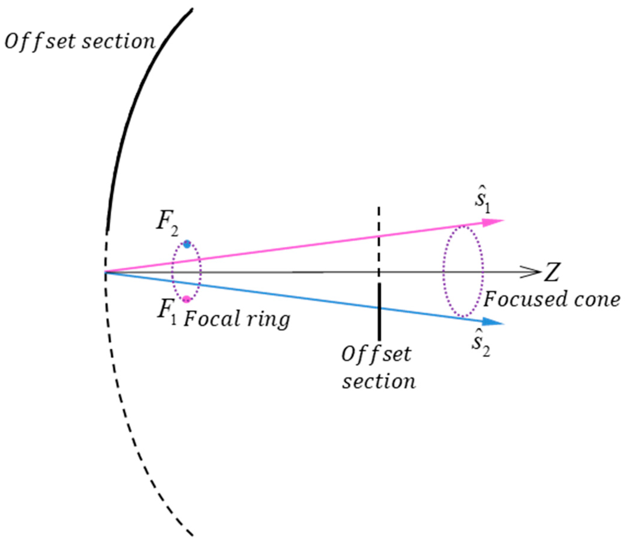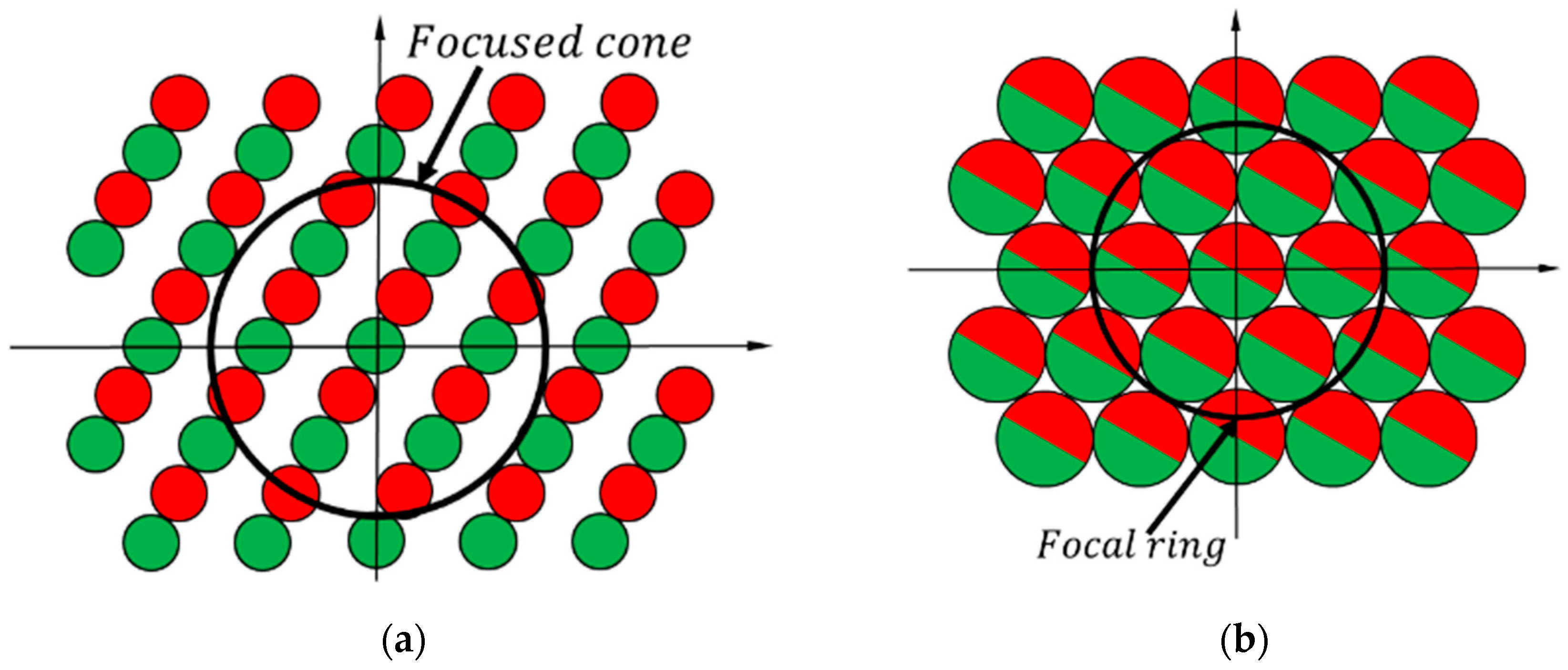The unit vectors ${\widehat{y}}_f$ and $\widehat{y}$, not represented, are normal to the plane of the figure. The main-RA will be supported by the same parabolic main reflector surface of the Cassegrain while two different options will be considered for the flat sub-RA. The first one is used to synthesize a bifocal configuration with a focal ring and a focused cone as shown in Figure 5. Since for this case the sub-RA surface must be symmetric about the Z axis, it must be normal to the Z axis (if a flat surface is required), otherwise it should be a curved surface. For instance, if a tilted section is chosen, the sub-RA would be a cone. 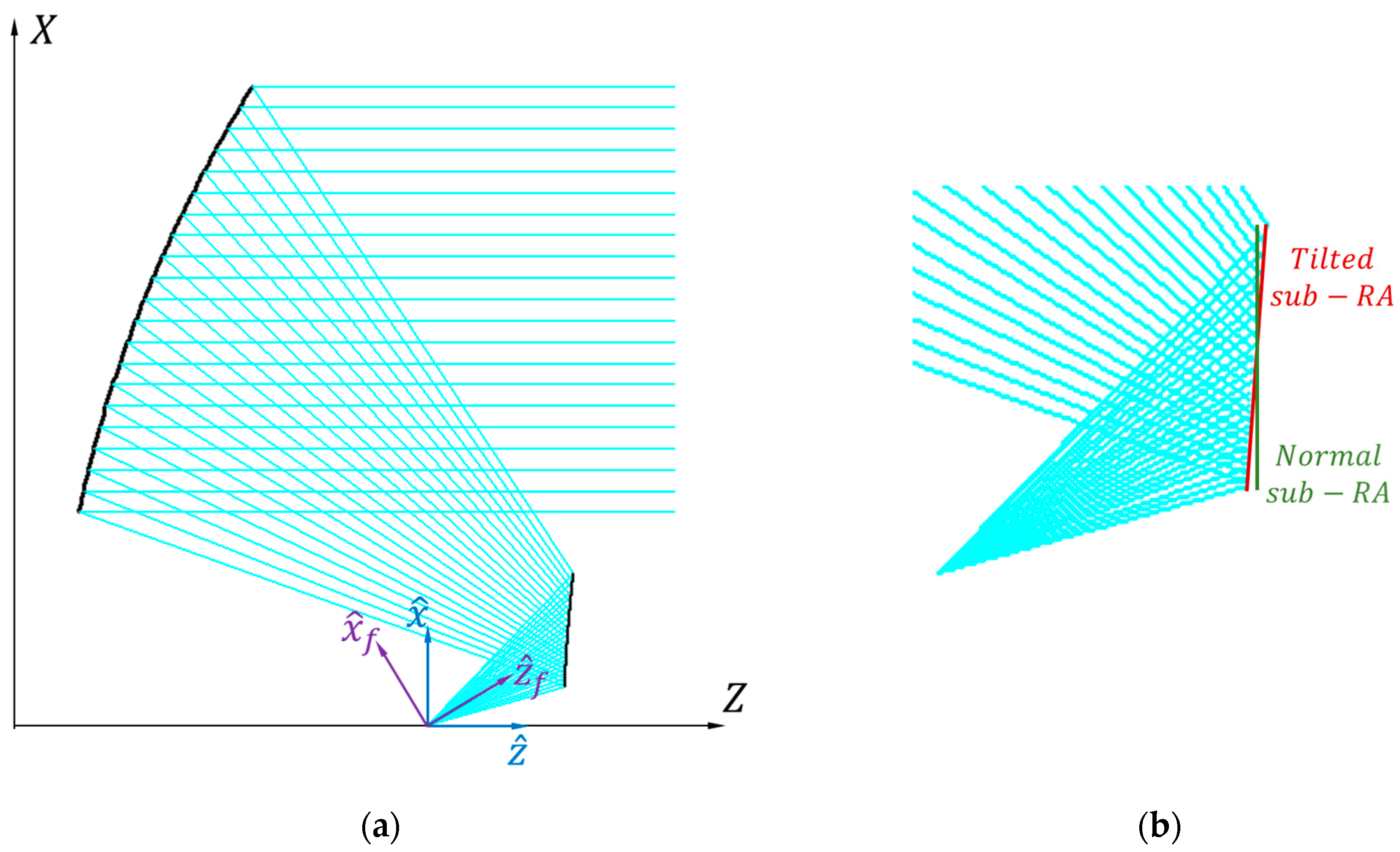The second option for the sub-RA is selected to synthesize a bifocal configuration with two focal points with the 3D extension shown in Figure 4. In this case, a tilted sub-RA plane is selected to be tangent to the hyperbolic surface at a central point adequately selected to reduce the average difference between the hyperbolic surface and the tangent plane. Both choices are depicted in Figure 6b.

The geometric parameters of the two baseline Cassegrain configurations are summarized in

Table 1. Baseline Cassegrain Parameters.

Geometric Parameter	Symbol and Value
Main reflector aperture diameter	D = 1.8 m
Main reflector focal length	f = 2.4 m
Main reflector offset heigth	hoff = 1.6 m (focal ring design) hoff = 1.8 m (Two foci design)
Inter-focal length	2c = 0.96 m
Feed location	Feed = (0, 0, −0.96) m
Magnification factor	M = 1.25

.

5.1. Focal Ring Bifocal Design

To achieve the desired scanning capability of the antenna, a focused cone with a central angle of 1.68° is enforced, along with a focal ring of radius 114 mm in the focal plane. This configuration ensures that the focused cone aligns with the map of beams, as shown in Figure 7, minimizing the mean scanning losses across the field of view. The map of beams depicted in Figure 7a shows two of the four colors which are necessary for the whole coverage by reusing two frequencies and two polarizations. Figure 7b shows schematically the cluster of feed apertures, each providing two beams. Two antennas would be necessary, each one providing two of the four colors. As can be seen in Figure 7b, the cluster of dual beams covers all the focal plane space, so a second antenna is necessary to provide the other two colors not represented in Figure 7a.

The sub-RA plane was selected to be normal to the Z axis (as shown in Figure 6b) and containing a central point of the original hyperbolic subreflector of the baseline Cassegrain configuration. The bifocal algorithm described in Section 4.1 was applied in the offset plane. The iterations of the algorithm started at the vertex of the parabola in the Z axis, generating a first set of data points. A second set of data points was obtained, as described in Section 4.1, starting from the vertex of the hyperbola in the Z axis. Due to the symmetry of the problem, only half of the data points (those corresponding to $x\ge 0$) were used to adjust the polynomial approximation $L\left(x\right)$, according to Appendix B, but without considering $z_y$, $\partial L/\partial y$ or $N_y$ since it is a 2D problem. The polynomial approximation was performed using the following basis functions:

$$\begin{gathered} L\left(x\right)=\sum _{n=0}^8{a}_n{\psi }_n\left(x\right), \frac{\partial L\left(x\right)}{\partial x}=\sum _{n=0}^8{a}_n{\psi }_n^{\prime }\left(x\right), \\ {\psi }_n\left(x\right)=x^n, {\psi }_n^{\prime }\left(x\right)=n{x}^{n-1}. \end{gathered}$$

(21)

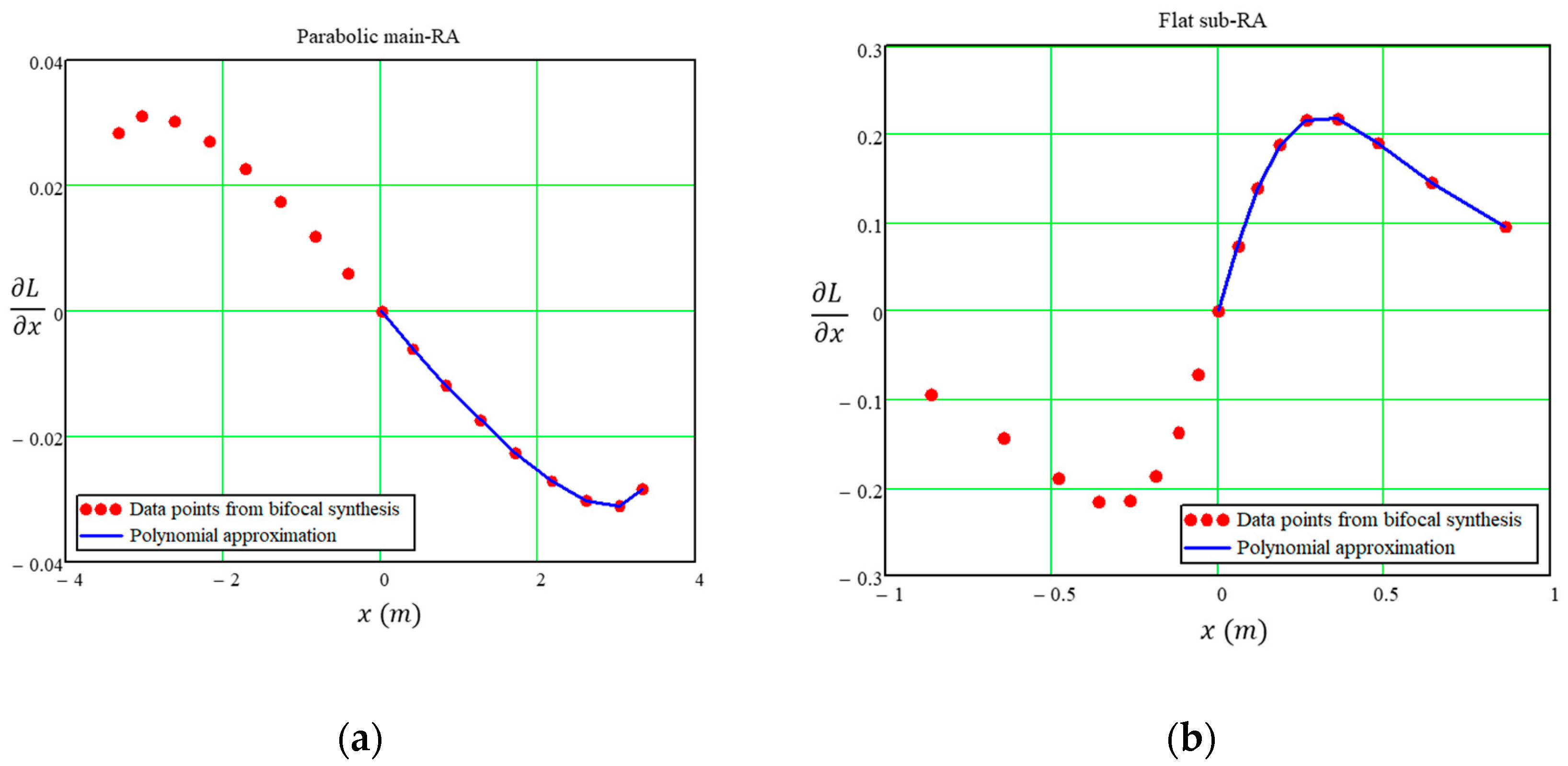
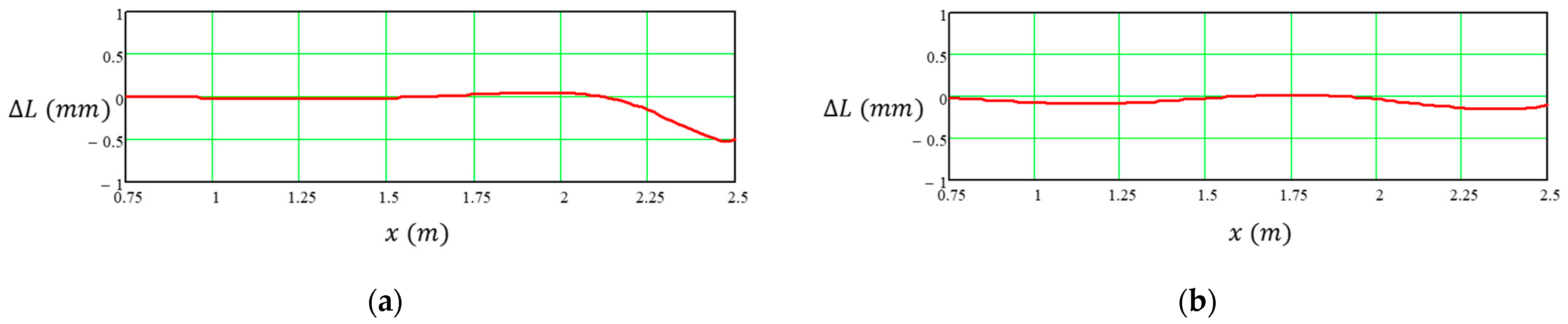
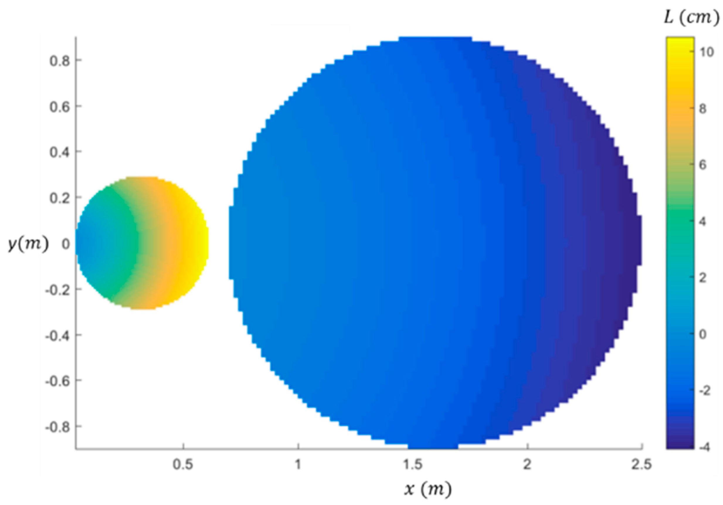
Figure 8 shows the derivative of L(x) as obtained from the bifocal synthesis algorithms through the computation of the virtual normal and the polynomial approximation used to characterize the reflectarrays. The maximum errors for these derivatives due to the polynomial approximation have been found to be less than 5 × 10⁻⁵ for the flat sub-RA and 2 × 10⁻⁵ for the parabolic main-RA. The global view of the path length shift $L(x,y)$ is depicted in Figure 9. It must be taken into account that the function $L$ is circularly symmetric, depending only on the radial cylindrical coordinate $\rho$.

The focusing properties have been evaluated by GO and the results are depicted in Figure 10. A quasi-perfect focusing is achieved when scanning to ±1.68° and the feed is located at the corresponding focal point. The case −1.68° is quite good, but in general, scanning to negative values in the offset plane is worse than the corresponding positive value because the upper part of the subreflector, where the asymmetry due to the offset configuration is steeper, is used.

Basic Physical Optics (PO) simulations at 20 GHz have been developed by using in-house software tools [15,16] based on discretizing the surface in small triangular patches. The implementation of the impact of the phase shift due to the reflectarrays has been performed by multiplying the currents predicted using PO by the phase shift term (proportional to the path length) computed at the center of each patch. Ideal feed models of cos-q type have been adopted, providing edge taper illumination of −12 dB. Figure 11 shows the PO patterns for the bifocal design with focal ring when the feed is located to make the antenna scan in the boresight direction and in the $\theta =1.68°$ for the principal cuts. The scanning behavior of the antenna is satisfactory. The lack of symmetry observed in the XZ plane is a result of the offset configuration employed in the design.

5.2. Bifocal Design with Two Focal Points

In this design, two focal points were selected to correspond to scanning directions at θ = 1.68° in the YZ plane (ϕ = 90° and ϕ = −90°). The focal points were chosen to replicate the same deviation factor as in the baseline Cassegrain design in order to maintain the size of the sub-RA. In this design, the sub-RA plane is the tilted version of Figure 6b, and a feed plane normal to the ${\widehat{z}}_f$ direction was considered. The ${\widehat{z}}_f$ direction points from the original feed point in the baseline Cassegrain to the bisector direction of the sub-RA. The two focal points were chosen in this feed plane by GO calculations in the baseline Cassegrain. Two sets of rays incoming to the main reflector from the focal directions (θ = 1.68°, ϕ = ±90°) are considered. After reflection of the sets of rays at main reflector and subreflector, the best focusing points at the feed plane are computed, providing the coordinates of the focal points at (0, −0.0952, −0.96) for ϕ = 90° and (0, 0.0952, −0.96) for ϕ = −90°.

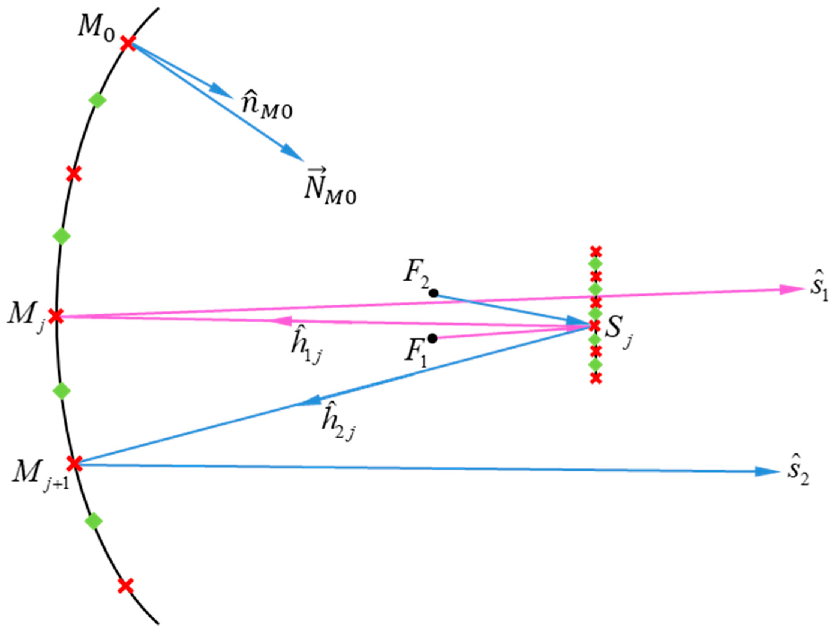
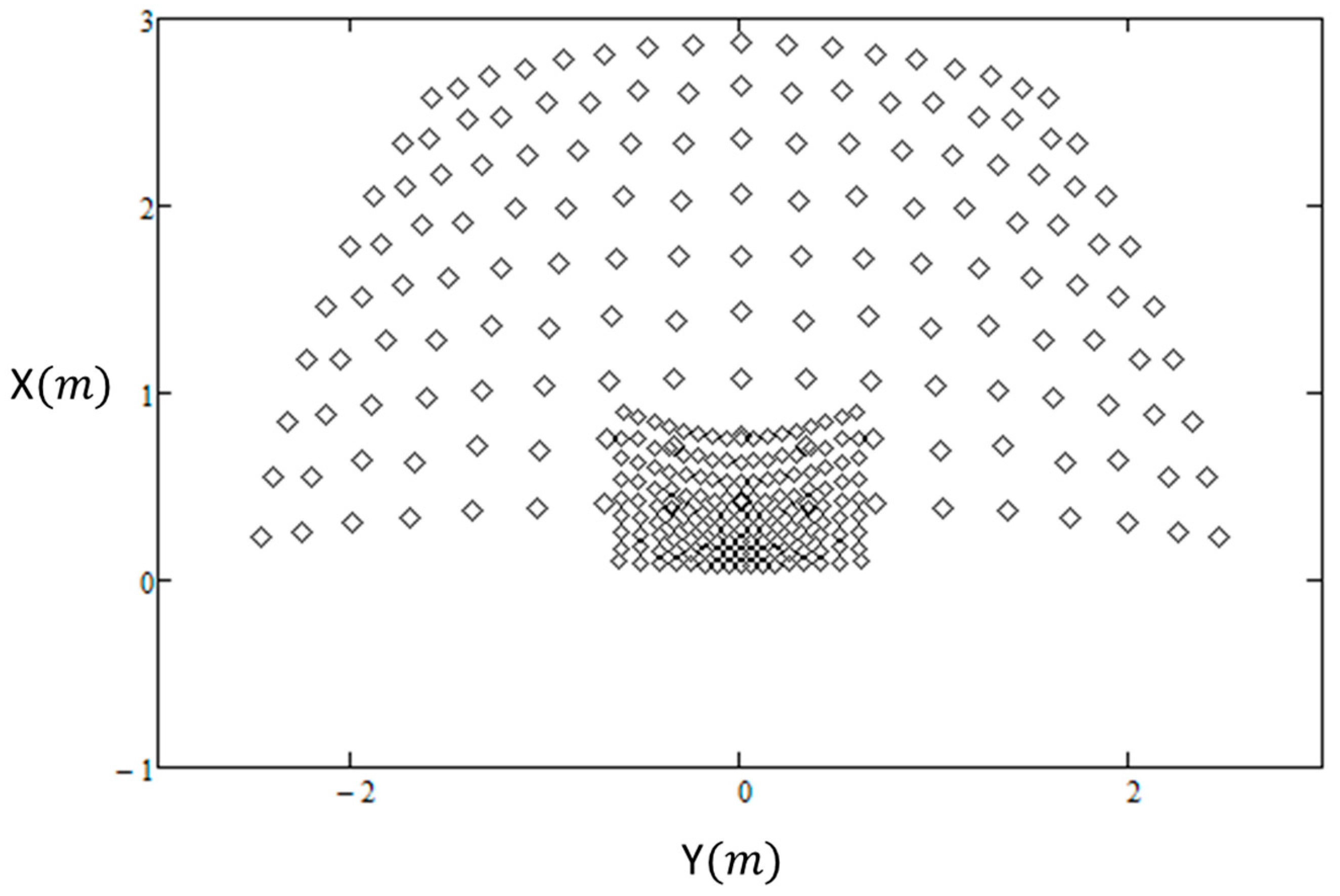
Before synthesizing the 3D main-RA and sub-RA as described in Section 4.2, a central section of the reflectarrays is synthesized in the offset ZX plane. A bifocal central section is initially synthesized with focal directions (θ = 1.68°, ϕ = 0° and 180°). In this case, the focal points are also taken in the feed plane at the coordinates (−0.084929, 0, −0.911868) for ϕ = 0° and (0.081149, 0, −1.00599) for ϕ = 180°. The set of data points from the central section is then used to extend the synthesis in 3D, resulting a set of data points as depicted in Figure 12.

With the synthesized sets of data for the derivatives of the path length shift for main-RA and sub-RA, a polynomial interpolation was constructed by using the following basis functions:

$$L\left(x,y\right)=\sum _{j=0}^2\sum _{i=0}^3{p}_{ij}{\psi }_{ij}\left(x,y\right), {\psi }_{ij}\left(x,y\right)=x^i{y}^{2j+1}$$

(22)

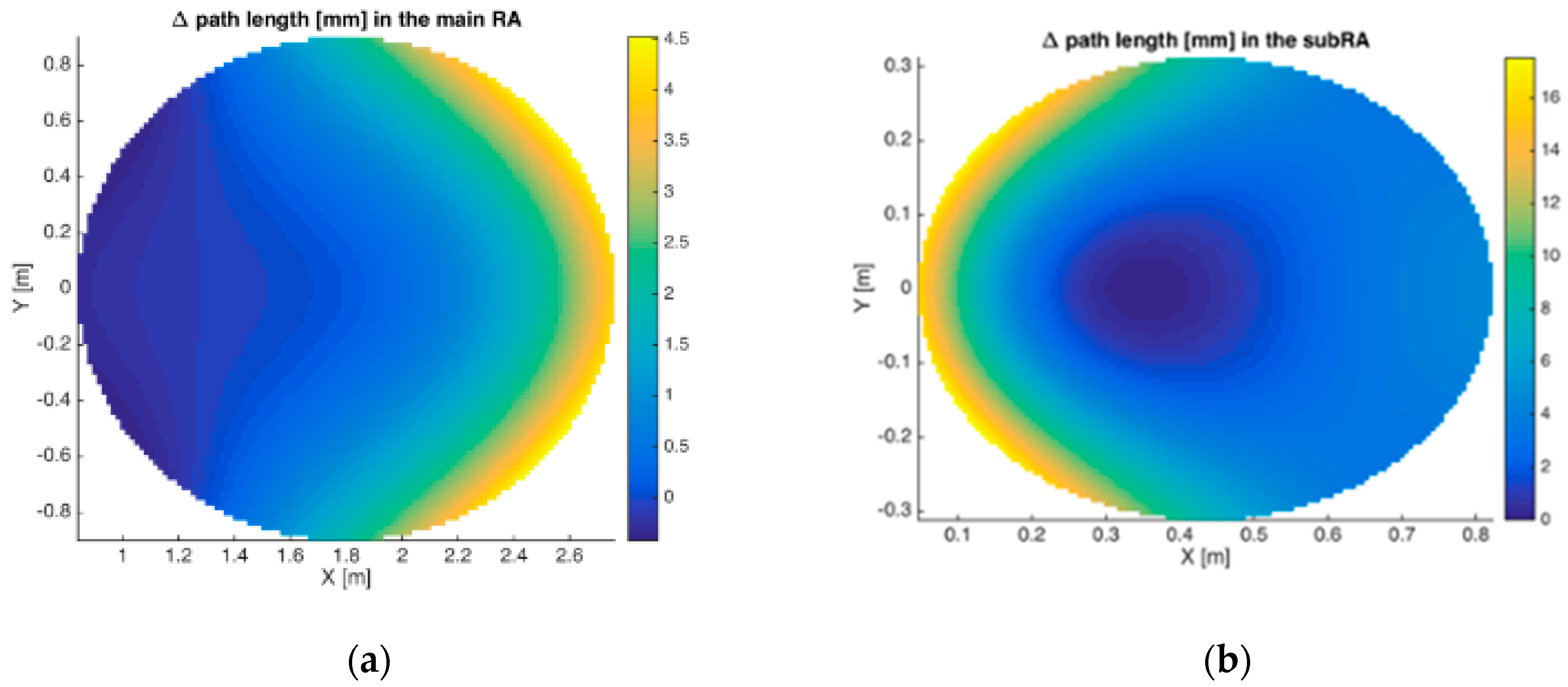
The data points used for interpolation exceed the area of the main-RA and sub-RA. This is convenient to improve the accuracy of the polynomial approximations. The view of the path length shift distribution and those of the phase delay distributions for both reflectarrays are plotted in Figure 13. It can be observed that a deeper variation in path length shift variation is required for the flat sub-RA than for the main reflector. The error due to the polynomial interpolation for the partial derivatives has been found to be less than 5 × 10⁻³ for the flat sub-RA and less than 2 × 10⁻³ for the main-RA.

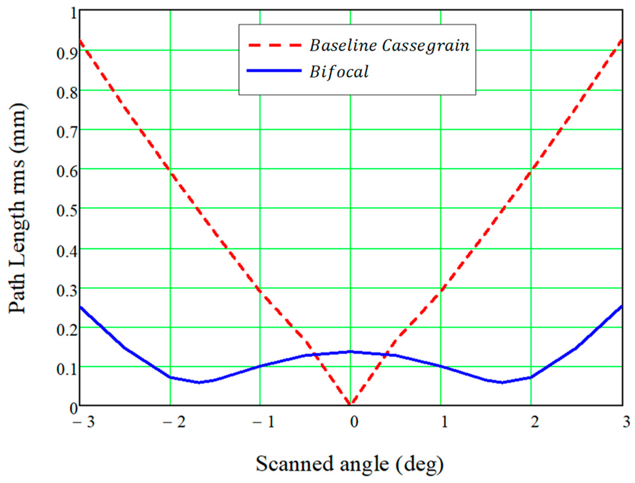
To verify the focusing properties of the designed bifocal dual reflectarray, the uniformity of the phase distribution across the scanned aperture was studied by analyzing the root mean square (rms) of the path length after GO simulations. Figure 14 compares the path length rms when the antenna scans in the plane of the foci compared to that of the baseline Cassegrain.

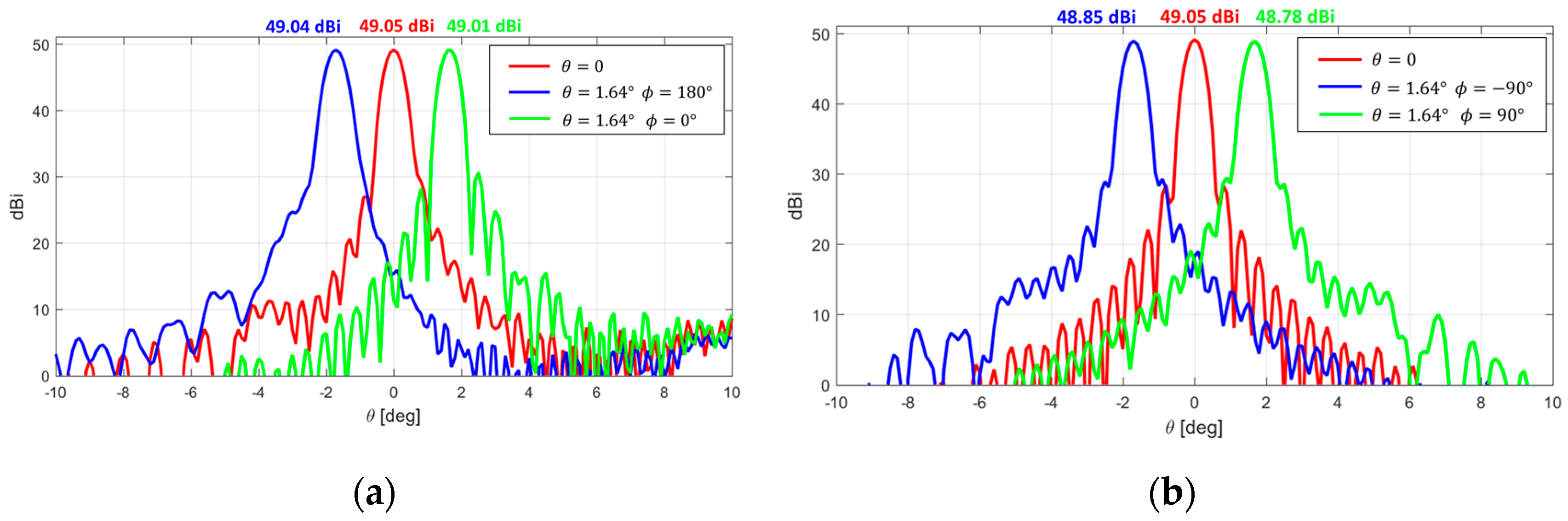
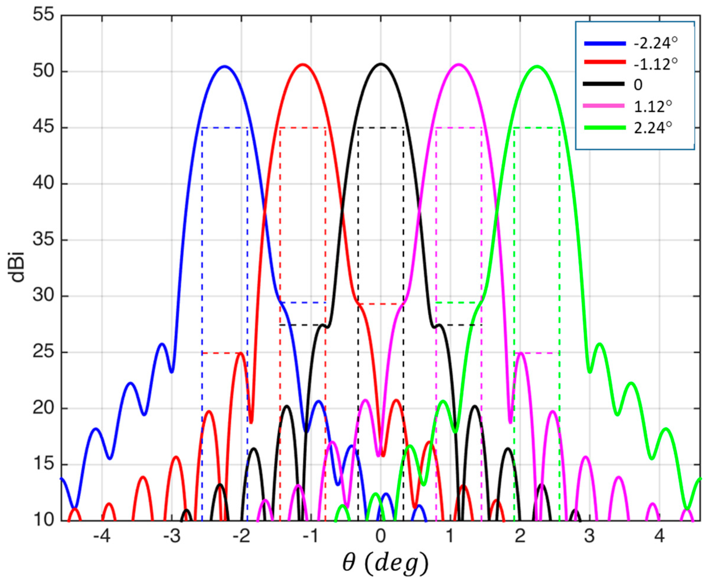
Again, basic Physical Optics (PO) simulations at 20 GHz were performed using the same approximations adopted in Section 5.1. Figure 15 show the Physical Optics patterns for the bifocal design with two foci when the antenna scans in the plane where the focusing directions are located. The maximum ripple of the gain for the considered beams, extending beyond the focal directions is approximately 0.2 dB compared to about 0.5 dB ripple observed in the baseline Cassegrain configuration.

6. Conclusions

In this paper, a novel vector formulation has been proposed for the synthesis of curved reflectarrays using ray tracing techniques. The concept of path length shift, which is directly proportional to the phase distribution, has been introduced and applied to solve the first stage of the reflectarray synthesis problem without restrictions in frequency. The concept of virtual normal, which characterizes the reflection law at the reflectarray surface, enables the vector formulation of ray tracing for curved reflectarrays. Equations have been developed to establish the relationship between the virtual normal, obtained in the GO synthesis, and the derivatives of the path length shift distribution with respect to the coordinates of the aperture of the curved reflectarray. The path length shift, and, hence, the phase distribution is then reconstructed by an interpolation scheme that is also presented. This interpolation minimizes, in a least mean squares sense, the differences between the synthesized derivatives of the path length shift, as obtained from the GO synthesis, and the derivatives of the interpolation polynomial.

Two different configurations of bifocal dual reflectarrays have been presented, along with numerical results that demonstrate the feasibility of the proposed solution. In the first configuration, a focal ring is generated in the focal plane, improving the antenna’s field of view when a cluster of feeds is used to achieve a multibeam antenna, as opposed to the standard case of having a single focal point. The reflectarray synthesis in this configuration is a 2D problem, and the 3D extension is obtained through the rotational symmetry of the phase shift synthesized using the bifocal technique in the central section of the surfaces. In the second configuration, a 3D synthesis problem is solved to produce two foci in the horizontal plane of the antenna, resulting in enhanced scanning performance in such plane.

References

1. Schneider, M.; Hartwanger, C.; Wolf, H. Antennas for multiple spot beams satellites. CEAS Space J. 2011, 2, 59–66. [Google Scholar] [CrossRef] [Green Version]
2. Rao, B.L. Bifocal dual reflector antenna. IEEE Trans. Antennas Propag. 1974, 22, 711–714. [Google Scholar] [CrossRef]
3. Rappaport, C. An offset bifocal reflector antenna design for wide-angle beam scanning. IEEE Trans. Antennas Propag. 1984, 32, 1196–1204. [Google Scholar] [CrossRef]
4. Pino, A.G.; Llombart, N.; González-Valdés, B.; Rubiños, O. A Bifocal Ellipsoidal Gregorian Reflector System for THz Imaging Applications. IEEE Trans. Antennas Propag. 2012, 60, 4119–4129. [Google Scholar] [CrossRef]
5. Martinez-de-Rioja, E.; Martinez-de-Rioja, D.; Encinar, J.A.; Pino, A.; Gonzalez-Valdes, B.; Rodriguez-Vaqueiro, Y.; Arias, M.; Toso, G. Advanced Multibeam Antenna Configurations Based on Reflectarrays: Providing Multispot Coverage with a Smaller Number of Apertures for Satellite Communications in the K and Ka Bands. IEEE Antennas Propag. Mag. 2019, 61, 77–86. [Google Scholar] [CrossRef]
6. Martinez-de-Rioja, E.; Encinar, J.A.; Pino, A.; Rodriguez-Vaqueiro, Y. Broadband Linear-to-Circular Polarizing Reflector for Space Applications in Ka-Band. IEEE Trans. Antennas Propag. 2020, 68, 6826–6831. [Google Scholar] [CrossRef]
7. Menzel, W.; Al-Tikriti, M.; Leberer, R. A 76 GHz multiple-beam planar reflector antenna. In Proceedings of the 32nd European Microwave Conference, Milan, Italy, 23–26 September 2002. [Google Scholar] [CrossRef]
8. Cuevas, J.G.; Tienda, C.; Encinar, J.A.; Krieger, G. Principle of bifocal antennas implemented in a dual reflectarray configuration. In Proceedings of the 9th European Conference on Antennas and Propagation (EUCAP), Lisbon, Portugal, 12–17 April 2015. [Google Scholar]
9. Martínez-de-Rioja, E.; Encinar, J.A.; Pino, A.; González-Valdés, B.; Hum, S.V.; Tienda, C. Bifocal Design Procedure for Dual-Reflectarray Antennas in Offset Configurations. IEEE Antennas Wirel. Propag. Lett. 2018, 17, 1421–1425. [Google Scholar] [CrossRef]
10. Leberer, R.; Menzel, W. A dual planar reflectarray with synthesized phase and amplitude distribution. IEEE Trans. Antennas Propag. 2005, 53, 3534–3539. [Google Scholar] [CrossRef] [Green Version]
11. Pino, A.; Rodríguez-Vaqueiro, Y.; González-Valdés, B.; Rubiños, O.; Martínez-de-Rioja, E.; Encinar, J.A.; Toso, G. Design of a Bifocal dual Reflectarray System with Parabolic Main Surface for a Multifed Space Antenna. In Proceedings of the IEEE International Symposium on Antennas and Propagation and USNC-URSI Radio Science Meeting (APS/URSI), Boston, MA, USA, 8–13 July 2018. [Google Scholar] [CrossRef]
12. Martinez-de-Rioja, D.; Martinez-de-Rioja, E.; Rodriguez-Vaqueiro, Y.; Encinar, J.A.; Pino, A. Multibeam Reflectarrays in Ka-Band for Efficient Antenna Farms Onboard Broadband Communication Satellites. Sensors 2021, 21, 207. [Google Scholar] [CrossRef] [PubMed]
13. Martinez-de-Rioja, E.; Encinar, J.A.; Toso, G. Bifocal Dual-Reflectarray Antenna to Generate a Complete Multiple Spot Beam Coverage for Satellite Communications in Ka-Band. Electronics 2020, 9, 961. [Google Scholar] [CrossRef]
14. Martínez-de-Rioja, D.; Martínez-de-Rioja, E.; Rodríguez-Vaqueiro, Y.; Encinar, J.A.; Pino, A.; Arias, M.; Toso, G. Transmit–Receive Parabolic Reflectarray to Generate Two Beams per Feed for Multispot Satellite Antennas in Ka-Band. IEEE Trans. Antennas Propag. 2021, 69, 2673–2685. [Google Scholar] [CrossRef]
15. Martínez, J.A.; Pino, A.G.; Vega, I.; Arias, M.; Rubiños, O. ICARA: Induced current analyis of reflector antennas. IEEE Antennas Propag. Mag. 2005, 47, 92–100. [Google Scholar] [CrossRef]
16. Arias-Acuña, M.; García-Pino, A.; Rubiños-López, O. Fast Far Field Computation of Single and Dual Reflector Antennas. J. Eng. 2013, 2013, 140254. [Google Scholar] [CrossRef] [Green Version]
Figure 1. Absolute system and local system for the reflectarray surface.
Electronics 12 02619 g001
Figure 2. Detail of incident and reflection angles, and ray vectors.
Electronics 12 02619 g002
Figure 3. Bifocal reflectarray synthesis algorithm for a linear section. Two procedures were applied based on the same algorithm to double the density of data points: starting at a known point M 0 on the main-RA to generate “×” points and starting at a known point S 0 on the sub-RA to generating “” points. Both procedures lead to the same geometry.
Electronics 12 02619 g003
Figure 4. Bifocal reflectarray 3D synthesis scheme. A central section in the plane of symmetry is first synthesized as “Starting profile”. Then, starting at each point of the starting profile, a lateral strip is synthesized allowing the 3D extension of the reflectarray surface. Crosses are obtained by starting at the main-RA central section while diamonds are obtained by starting at sub-RA central section. The left part, not represented in the figure, is obtained by symmetry means.
Electronics 12 02619 g004
Figure 5. Bifocal 3D extension by rotation about the Z axis.
Electronics 12 02619 g005
Figure 6. Baseline Cassegrain: (a) General view and ray tracing; (b) Detail of flat sub-RA.
Electronics 12 02619 g006
Figure 7. Multibeam configuration for one antenna (two are necessary for whole coverage): (a) map of beams, each color represents a different polarization; (b) feed cluster where each antenna generates two beams with perpendicular polarizations.
Electronics 12 02619 g007
Figure 8. Derivatives of L ( x ) for the focal ring bifocal: (a) main-RA; (b) sub-RA.
Electronics 12 02619 g008
Figure 9. Path length shift distribution across the reflectarrays.
Electronics 12 02619 g009
Figure 10. Ripple of the path length shift ( L ) across the main-RA aperture when scanning: (a) to −1.68°; (b) to +1.68°.
Electronics 12 02619 g010
Figure 11. PO patterns at 20 GHz: (a) XZ cut; (b) YZ cut.
Electronics 12 02619 g011
Figure 12. Set of data points obtained for the synthesis of the bifocal dual reflectarray.
Electronics 12 02619 g012
Figure 13. Path length shift of the bifocal dual reflectarray with two focal points: (a) main-RA; (b) sub-RA.
Electronics 12 02619 g013
Figure 14. Path length rms of the scanned aperture for the bifocal and the Cassegrain.
Electronics 12 02619 g014
Figure 15. Physical Optics patterns for the bifocal design with two foci. Dotted lines depict masks of requirements for main lobe and side lobes.
Electronics 12 02619 g015