Data Fusion and Situation Awareness for Smart Grid and Power Communication Network Based on Tensor Computing and Deep Reinforcement Learning

Abstract

With the large-scale deployment of sensors, both the smart grid and the power communication network should jointly deal with different kinds of big data. The fusion of both networks should bring unpredictable accidents, even leading a catastrophic destruction in our lives. However, data fusion (DF) and coordination treatment for two networks will greatly improve system performance, reduce system complexity, and improve the precision and control ability of both networks. Situation awareness (SA) is the key function for DF and accident avoidance for both networks with different network structures, data types, system mechanisms, and so on. This paper use tensor computing to provide a general data model for heterogeneous and multidimensional big data generated from smart grid and power communication network. A novel data fusion scheme is designed with multidimensional tensors. Deep reinforcement learning (DRL) algorithms are utilized to construct an optimal SA strategy based on tensor big data. A multi-agent actor-critic (MAAC) algorithm is used to achieve an optimal SA policy and improve system performance. The proposed DF and SA schemes based on tensor computing and DRL provide useful guidance for smart grid and power communication networks from theory and practice.

1. Introduction

1.1. Smart Grid Based on 5G Networks

The smart grid is a novel power grid, which combines advanced sensing and measurement technologies, information and communication technologies, analysis and decision technologies, automatic control and intelligent power technologies, and is highly integrated with power grid infrastructures [1,2,3]. The 5G networks, with their characteristics of large bandwidth, wide connection, low delay, and high reliability, combined with innovative technologies, such as network slicing and edge computing, can well meet the communication requirements of a smart grid. 5G applications based on existing power grid services, such as distribution network differential protection, millisecond precision load control, low delay, large bandwidth, and security protection, are in urgent need of communication reliability. 5G technologies provide a foundation for the promotion and application of these services [4,5]. On the basis of the traditional power grid, the smart grid integrates advanced technologies, such as communication and sensing measurement, to form a new type of power grid, which represents the developing trends of future power grids. In a smart grid, the information and communication technology (ICT) infrastructure makes physical infrastructure more efficient, ensures secure integration of more renewable energy, and smart devices guarantee self-healing capabilities and efficient power supply and allow customers more control over their electricity consumption. As an important support for the power system’s safe, stable, and efficient operation, the communication information system runs through every application link. Under the current trend of smart grid development, the completion and improvement of communication information systems will realize the comprehensive collection and efficient processing of various production, operation, and service information and realize the optimal allocation and efficient utilization of grid resources.

1.2. Power Communication Network

The power communication network is a special communication network formed with the power system. It is an important infrastructure to provide data transmission for electric power dispatching and production. The power communication network is developed to ensure the safe and stable operation of the power system; it is the basis of the automation of power grid dispatching, network operation marketization, and management modernization [6,7]. With the increasing scale and complexity of the power communication network, the operation and monitoring task is becoming more and more difficult, which poses new challenges for the data management innovation of power-related business. At the same time, the dependence and coupling between the power communication network and the smart grid are gradually deepened, which greatly improves the flexibility, observability, and controllability of the power system. This connection brings positive significance for maintaining the safe and stable operation of the power network under abnormal conditions.

Power communication networks can analyze the health of transmission lines by collecting data from multiple sensors. In real applications, data loss and anomalies often occur in terminal sensors due to bad weather, natural disasters, and sensor interference. Therefore, a new data fusion (DF) model can be developed to compensate for missing data and outliers, eliminate potential risks to the network, and improve the reliability of communication [8,9]. The power communication network can not only provide a communication guarantee with information resources but also lead to a greater threat of power system instability. In view of these problems, it is urgent to study and analyze the vulnerability of the power grid caused by the interdependent coupling between the smart grid and the power communication network.

1.3. Data Fusion and Situation Awareness Based on Tensor Computing and Deep Reinforcement Learning

Situation awareness (SA) is used to sense current situations of the smart grid and power communication network from DF. When the current situations of both networks are sensed, the potential operating risks can be estimated or predicted [10,11,12].

DF has the characteristics of big data generated from both the smart grid and the power communication network with heterogeneous and multidimensional data [13,14]. Tensor computing provides an efficient way to deal with big data, which are compacted in a single data tensor [15]. The tensor completion scheme can be used to complete imperfect tensor big data. The tensor decomposition scheme can be used to decompose tensor big data from different dimensions, such as time, frequency, energy, and so on. The tensor decomposition scheme provides an important way to analyze tensor big data from specific dimensions. Moreover, the tensor eigenvalue also provides a possible way to estimate some key performances of tensor big data [16,17,18,19]. With the big data generated from the smart grid and power communication network, the whole system should achieve an optimal SA scheme to perceive the complicated situations from both systems. DRL is a sharp tool to achieve an optimal SA policy [20]. DRL combines deep learning and reinforcement learning and has the advantages of both sides, with the ability to provide strong perceptions and decision-making.

Here, DRL trains and achieves an optimal awareness scheme offline based on tensor big data and DF. The main contributions of the paper can be summarized as follows:

• A novel DF scheme based on tensor theory is designed for both smart grids and power communication networks. The heterogeneous and multidimensional big data of both networks can be compacted in a tensor, leading to an efficient big data processing scheme. For the proposed DF scheme, the tensor completion and tensor decomposition algorithms are used to deal with sparse big data.
• The deep reinforcement learning scheme is used to fulfill the SA scheme, in which a new multi-agent actor-critic (MAAC) algorithm is proposed to learn and train the optimal SA scheme.
• We combine a new DF scheme and SA scheme for both networks, leading to a novel and efficient information processing scheme for future smart grid and intelligent power communication networks.

The remainder of the paper is provided as follows. Section 2 introduces the system model and provides the problem of DF and SA. Section 3 introduces the key concept of tensor computing and provides an efficient DF scheme based on tensor computing. Section 4 provides the SA scheme based on deep reinforcement learning. The MAAC algorithm is proposed to design an optimal SA policy. Section 5 provides simulation results with theoretical analysis. In Section 6, the paper is concluded.

2. System Model and Problem Formulation

In this section, we first describe the system model based on the smart grid and power communication network. In the target system, two networks are analyzed. Then the SA problem is considered, where the smart grid and the power communication network are integrated, and big data are generated from both networks. The heterogeneous and multidimensional big data is processed by the DF scheme.

2.1. System Model

The system model based on 5G systems is shown in Figure 1, where the smart grid and the power communication network work together. The smart grid provides the power supply, and the corresponding power communication network provides information transmission. The smart grid has a flexible infrastructure, where energy sources for power generation are various. In addition to traditional thermal power generation, there is wind power, hydropower, solar power, etc. Unlike the one-way flow of the conventional power grid, the smart grid generation can also happen on the client side, such as photovoltaic power generation, as shown in Figure 1. The power goes through power transmission, power transformation, power distribution, and ultimately to the customers. At the same time, the power communication systems integrated with the smart grid provide communication service to the power supply side and customer side. As shown in Figure 1, the power lines (red lines) and the communication links (black lines) can form one integrated network, where two different kinds of data should be processed efficiently, and the operation situation should be sensed. Different kinds of sensors from the smart grid and the power communication network generate varying kinds of data, leading to an integrated heterogeneous network structure. Therefore, an efficient DF scheme should be developed to deal with different kinds of big data.

2.2. Data Fusion and Situation Awareness

Different kinds of sensors of two networks can generate different kinds of big data. The whole system based on the smart grid and the power communication network shown in Figure 1 should process those big data. A DF center should be constructed, and an efficient DF scheme should be designed. The DF scheme can be simply formulated as

$$\mathcal{D}=\mathrm{F}\left(\mathcal{S},\mathcal{C}\right)$$

(1)

where the fused data, the smart grid data, and the communication data are denoted by three big data tensors $\mathcal{D}$, $\mathcal{S}$, and $\mathcal{C}$, respectively. The fused data $\mathcal{D}\in {\mathbb{R}}^{I_1\times I_2\times \cdots \times I_N}$ denote an N-dimension tensor with N dimensions $I_1\times I_2\times \cdots \times I_N$. The fused data $\mathcal{D}$ can be considered as a multidimensional data container with a given format. The big data of the smart grid is denoted by an M-dimension tensor $\mathcal{S}\in {\mathbb{R}}^{I_1\times I_2\times \cdots \times I_M}$, which can compact the big data from the smart grid. Following the same way, the big data of the power communication network is denoted by a K-dimension tensor $\mathcal{C}\in {\mathbb{R}}^{I_1\times I_2\times \cdots \times I_K}$. The fusion function is denoted by $\mathrm{F}\left(:,:\right)$, which is used to combine and unify two kinds of big data. SA, also named situation (state) sensing, is the key function to managing, monitoring, and predicting system situations of the smart grid and the power communication network. A large amount of data captured from both networks can support SA in terms of system performance, such as quality of service (QoS), system parameters, stable voltage, energy efficiency, and so on. Note that SA here mainly indicates the operation state of both networks. Traditional SA scheme is outdated and inefficient due to lots of artificial operations and suboptimal algorithms. Therefore, based on the fused big data, we should develop an optimal and efficient SA scheme. Deep reinforcement learning provides a potential way to develop and train a novel SA scheme to identify and estimate demand response, power patterns, and potential risks in both networks.

3. Data Fusion Based on Tensor Computing

Tensor computing provides an efficient way of data fusion, which is based on the data structure of tensor as shown in (1). The big data from the smart grid and the power communication network are both dealt with in the format of tensors. Due to practical reasons, the tensor big data is sometimes sparse or incomplete. The tensor completion scheme is used to complete sparse tensor big data. In order to generate the fused data $\mathcal{D}$, the tensor decomposition scheme is used to analyze the target tensor big data from a specific dimension.

3.1. Preliminary of Tensor Computing

Here the tensor is defined as a multidimensional array. More precisely, an Nth-order or N-way tensor is an element of N vector spaces defined by the tensor product, each of which has its own coordinate system. This notion of a tensor is not equal to tensors in physics and chemistry, such as stress, and is always termed as a tensor field in mathematics. The concept of tensors is a generalization of vectors or matrices. A first-order tensor is a vector, a second-order tensor is a matrix, and tensors of order three or more are called higher-order tensors. An N-way tensor $\mathcal{X}\in {\mathbb{R}}^{I_1\times I_2\times \cdots \times I_N}$ is rank-one if and only if it can be written as the outer product of N vectors, i.e., $\mathcal{X}={\mathbf{a}}^{\left(1\right)}\circ {\mathbf{a}}^{\left(2\right)}\circ \cdots \circ {\mathbf{a}}^{\left(N\right)}$, where ${\mathbf{a}}^{\left(i\right)}$ denotes a i-length vector. Tensor matricization, expressed as unfolding, is the process of reordering the elements of a tensor into a matrix. The mode-n matricization of a tensor $\mathcal{X}\in {\mathbb{R}}^{I_1\times I_2\times \cdots \times I_N}$ is denoted by ${\mathbf{X}}_{\left(n\right)}$ and arranges the mode-n vectors to be the columns of the unfolding matrix. Tensors can be multiplied, and it is obvious that the product of tensors is much more complex than matrices. Here we just consider the tensor n-mode product rather than a full treatment of tensor multiplication. The n-mode (matrix) product of a tensor $\mathcal{X}\in {\mathbb{R}}^{I_1\times I_2\times \cdots \times I_N}$ with a matrix $\mathbf{A}\in {\mathbb{R}}^{J\times I_n}$ is denoted by $\mathcal{X}{\times }_n\mathbf{A}$ and is of size $I_1\times \cdots \times I_{n-1}\times J\times I_{n+1}\times \cdots \times I_N.$ Elementswise, we have

$${\left(\mathcal{X}\times {}_n\mathbf{A}\right)}_{i_1\cdots i_{n-1}j{i}_{n+1}\cdots i_N}=\sum _{i_n=1}^{I_n}{x}_{i_1{i}_2\cdots i_N}{a}_{j{i}_n}$$

(2)

where $x_{i_1{i}_2\cdots i_N}$ is the element of $\mathcal{X}$ and $a_{j{i}_n}$ denotes the $(j,i_n)$-the element of $\mathbf{A}$.

3.2. Tensor Decomposition

Tensor decomposition can be achieved by matrix singular value decomposition (SVD) and be utilized in the field of principal component analysis (PCA); that is, it can be considered as a higher-order generalization of matrix decomposition. Tensor decomposition can solve the dimensional disaster problem so as to fulfill dimensionality reduction processing, missing data filling, and implicit relationship mining. However, this method will make the structural information of the data lost, and the use of tensors to store the data can retain the structural information of the data. Two common decompositions in tensor decomposition are the Canonical Polyadic Decomposition (CPD) and the Tucker decomposition.

3.2.1. Cp Decomposition

The CPD is a form of decomposing arbitrary higher-order tensors into sums of multiple rank-one tensors. Take the third-order tensor $\mathcal{X}\in {\mathbb{R}}^{I_1\times I_2\times I_3}$ as an example; the CPD of the tensor can be written as

$$\mathcal{X}=\sum _{r=1}^R{\mathit{a}}_r\circ {\mathit{b}}_r\circ {\mathit{c}}_r$$

(3)

where R is the size of tensor rank, ${\mathit{a}}_r\in {\mathbb{R}}^{I_1},{\mathit{b}}_r\in {\mathbb{R}}^{I_2},{\mathit{c}}_r\in {\mathbb{R}}^{I_3}$, the operation “∘” denotes the vector outer product. The decomposition expression is concise, but the solution for rank is an NP-hard problem. The matrix composed of vectors that make up rank-one tenors is called the factor matrix under CPD, such as $\mathbf{A}=\left[a_1,a_2,a_3\dots a_R\right]$, the factor matrix $\mathbf{B}$ and $\mathbf{C}$ are defined the same. The CPD in matrix form can be written as

$$\begin{array}{c}\hfill {\mathbf{X}}_{\left(\mathbf{1}\right)}\approx \mathbf{A}{(\mathbf{C}\odot \mathbf{B})}^T\end{array}$$

(4)

$$\begin{array}{c}\hfill {\mathbf{X}}_{\left(\mathbf{2}\right)}\approx \mathbf{B}{(\mathbf{C}\odot \mathbf{A})}^T\end{array}$$

(5)

$$\begin{array}{c}\hfill {\mathbf{X}}_{\left(\mathbf{3}\right)}\approx \mathbf{C}{(\mathbf{B}\odot \mathbf{A})}^T.\end{array}$$

(6)

The CPD can usually be more simply written as follows

$$\mathcal{X}\approx \left[[\mathit{A},\mathit{B},\mathit{C}]\right]\equiv \sum _{r=1}^R{\mathit{a}}_r\circ {\mathit{b}}_r\circ {\mathit{c}}_r.$$

(7)

Taking the third-order tensor $\mathcal{X}\in {\mathbb{R}}^{\mathrm{I}\times \mathrm{J}\times \mathrm{K}}$ as an example, the goal of the algorithm is to calculate a CPD containing R rank-one tensors, so that it is as close as possible to the actual tensor, i.e.,

$$\underset{\widehat{\mathcal{X}}}{min}\parallel \mathcal{X}-\widehat{\mathcal{X}}\parallel \mathrm{with}\widehat{\mathcal{X}}=\sum _{r=1}^R{\lambda }_r{\mathbf{a}}_r\circ {\mathbf{b}}_r\circ {\mathbf{c}}_r=\left[[\mathit{\lambda };\mathbf{A},\mathbf{B},\mathbf{C}]\right].$$

(8)

3.2.2. Tucker Decomposition

Tucker decomposition was first proposed as a generalization of PCA in high dimensions. The model for the Tucker decomposition of the third-order tensor is

$$\mathcal{X}\approx \mathcal{G}{\times }_1\mathbf{A}{\times }_2\mathbf{B}{\times }_3\mathbf{C}=\sum _{\mathrm{p}=1}^{\mathrm{P}}\sum _{\mathrm{q}=1}^{\mathrm{Q}}\sum _{\mathrm{r}=1}^{\mathrm{R}}{\mathrm{g}}_{\mathrm{pqp}}{\mathbf{a}}_{\mathrm{p}}\circ {\mathbf{b}}_{\mathrm{q}}\circ {\mathbf{c}}_{\mathrm{r}}=\left[[\mathcal{G};\mathbf{A},\mathbf{B},\mathbf{C}]\right]$$

(9)

where $\mathcal{G}$ denotes the core tensor and $\mathbf{A}$, $\mathbf{B}$, and $\mathbf{C}$ are three matrices from three dimensions. The scalar form is expressed as

$${\mathcal{X}}_{\mathrm{ijk}}\approx \sum _{\mathrm{p}=1}^{\mathrm{P}}\sum _{\mathrm{q}=1}^{\mathrm{Q}}\sum _{\mathrm{r}=1}^{\mathrm{R}}{\mathrm{g}}_{\mathrm{pqr}}{\mathbf{a}}_{\mathrm{ip}}{\mathbf{b}}_{\mathrm{jq}}{\mathbf{c}}_{\mathrm{kr}},\mathbf{i}=1\dots \mathrm{I};\mathrm{j}=1\dots \mathrm{J};\mathrm{k}=1\dots \mathrm{K}$$

(10)

where $\mathbf{A}\in {\mathbb{R}}^{\mathrm{I}\times \mathrm{P}},\mathbf{B}\in {\mathbb{R}}^{\mathrm{J}\times \mathrm{Q}},\mathbf{C}\in {\mathbb{R}}^{\mathrm{K}\times \mathrm{R}}$. When $\mathrm{P}=\mathrm{Q}=\mathrm{R}$ and the kernel tensor is a supersymmetric tensor, the Tucker decomposition degenerates into the CPD. One of Tucker decomposition algorithms is indicated in Algorithm 1:

Algorithm 1 Tucker decomposition algorithm

1: for n = 1, …, N do 2:     ${\mathbf{A}}^{\left(n\right)}$ = left singular vectors of ${\mathbf{X}}_{\left(n\right)}$ 3:     $\mathcal{G}=\mathcal{X}\times {}_1{\mathbf{A}}^{\left(1\right)\top }\times {}_2{\mathbf{A}}^{\left(2\right)\top }\cdots {\times }_N{\mathbf{A}}^{\left(N\right)\top }$ 4:     return $\mathcal{G},{\mathbf{A}}^{\left(1\right)},{\mathbf{A}}^{\left(2\right)},\dots ,{\mathbf{A}}^{\left(N\right)}$ 5: end for

3.3. Tensor Completion

In reality, due to the limitation of data collection faults and other abnormal conditions, there are parts of missing data in the big data, which are called missing values. The repair of these missing values is called completion, and the estimation of missing values in the tensor domain is tensor completion. The core problem of missing data estimation is how to construct the relationship between missing values and observed values. Tensor completion is based on the impact of existing data on missing values and the low-rank assumption, which is mainly divided into two types of methods: one is based on the given rank and update factor in tensor completion; the other is to directly minimize the tensor rank and update the low-rank tensors. In the following, we take a third-order tensor completion problem as an example to introduce a special tensor completion algorithm named HaLRTC (high accuracy low rank tensor completion). Similar to matrix completion, given a sparse tensor $\mathcal{X}$ of size $n_1\times n_2\times n_3$, the index set corresponding to the observed elements is denoted as $(i,j,k)\in \Omega$. Let the tensor $\mathcal{S}$ of the same size be a binary tensor composed of elements 0 and 1, and satisfy $s_{ijk}=1,(i,j,k)\in \Omega$, otherwise $s_{ijk}=0,(i,j,k)\notin \Omega$. The objective function of the tensor completion problem can be written in the following format

$$\underset{\widehat{\mathcal{X}},{\mathcal{A}}_1,{\mathcal{A}}_2,{\mathcal{A}}_3}{min}{\alpha }_1{∥{\mathcal{A}}_{1\left(1\right)}∥}_{*}+{\alpha }_2{∥{\mathcal{A}}_{2\left(2\right)}∥}_{*}+{\alpha }_3{∥{\mathcal{A}}_{3\left(3\right)}∥}_{*}$$

(11)

where $\widehat{\mathcal{X}}$ represents the estimation of the original tensor $\mathcal{X}$, the magnitude of tensors ${\mathcal{A}}_1$, ${\mathcal{A}}_2$, ${\mathcal{A}}_3$ are $n_1\times n_2\times n_3$, the matrix ${\mathcal{A}}_{1\left(1\right)}$ with the magnitude of $n_1\times \left(n_2{n}_3\right)$ represents the mode-1 unfolding of tensor ${\mathcal{A}}_1$ under mode-1 unfolding and the matrix ${\mathcal{A}}_{2\left(2\right)}$ represents the mode-2 unfolding of ${\mathcal{A}}_2$, and the matrix ${\mathcal{A}}_{3\left(3\right)}$ represents the mode-3 unfolding of ${\mathcal{A}}_3$. In the objective function, the symbol ${∥·∥}_{*}$ represents the trace norm. The parameters ${\alpha }_1$, ${\alpha }_2$, ${\alpha }_3$ need to satisfy ${\alpha }_1+{\alpha }_2+{\alpha }_3=1$. There are two constraints of the optimization model. The first is to ensure that the elements of the estimated tensor $\widehat{\mathcal{X}}$ and the original tensor $\mathcal{X}$ on the set $\Omega$ are equal. The second is to set the intermediate variables ${\mathcal{A}}_1$, ${\mathcal{A}}_2$, and ${\mathcal{A}}_3$ equal to the estimated tensors. The constraints are given as follows

$$\left\{\begin{array}{c}\mathcal{S}\ast \widehat{\mathcal{X}}=\mathcal{S}\ast \mathcal{X}\hfill \\ \widehat{\mathcal{X}}={\mathcal{B}}_q,q=1,2,3\hfill \end{array}\right..$$

(12)

The HaLRTC algorithm is indicated in Algorithm 2:

Algorithm 2 HaLRTC algorithm

1: Input $\overrightarrow{\alpha }=\left({\alpha }_1,{\alpha }_2,{\alpha }_3\right)$, adaptively changing $\rho$ and maximum number of iterations K. 2: Initialize estimated tensor $\widehat{\mathcal{X}}$ that ${\widehat{x}}_{ijk}=\left\{\begin{array}{c}{x}_{ijk},(i,j,k)\in \Omega \hfill \\ 0,(i,j,k)\notin \Omega \end{array}\right.$, and attached zero tensor ${\mathcal{Y}}_1,{\mathcal{Y}}_2,{\mathcal{Y}}_3\in {\mathbb{R}}^{n_1\times n_2\times n_3}$. 3: Let k = 1. 4: Update ${\mathcal{B}}_q$: ${\mathcal{B}}_q={fold}_q\left\{D_{\frac{{\underline{\alpha }}_q}{\rho }}\left({\widehat{\mathcal{X}}}_{\left(q\right)}+\frac{1}{\rho }{\mathcal{Y}}_{q\left(q\right)}\right)\right\},q=1,2,3$, next; ($D_{\frac{{\alpha }_q}{\rho }}\left(X\right)=U{\Sigma }_{\frac{{\alpha }_q}{\rho }}{V}^T$). 5: Update $\widehat{\mathcal{X}}$: $\widehat{\mathcal{X}}=(1-\mathcal{S})\ast \left\{\frac{1}{3}{\sum }_{q=1}^3\left({\mathcal{B}}_q-\frac{1}{\rho }{\mathcal{Y}}_q\right)\right\}+\mathcal{S}\ast \mathcal{X}$. 6: Update ${\mathcal{Y}}_q$: ${\mathcal{Y}}_q={\mathcal{Y}}_q-\rho \left({\mathcal{B}}_q-\widehat{\mathcal{X}}\right),q=1,2,3$. 7: If $k<K,k=k+1$, return to step 4, else return estimated tensor $\widehat{\mathcal{X}}$. 8: End.

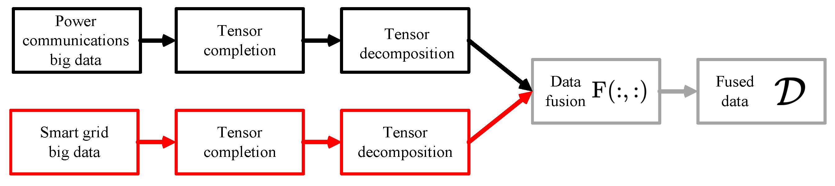
3.4. Tensor Based Data Fusion

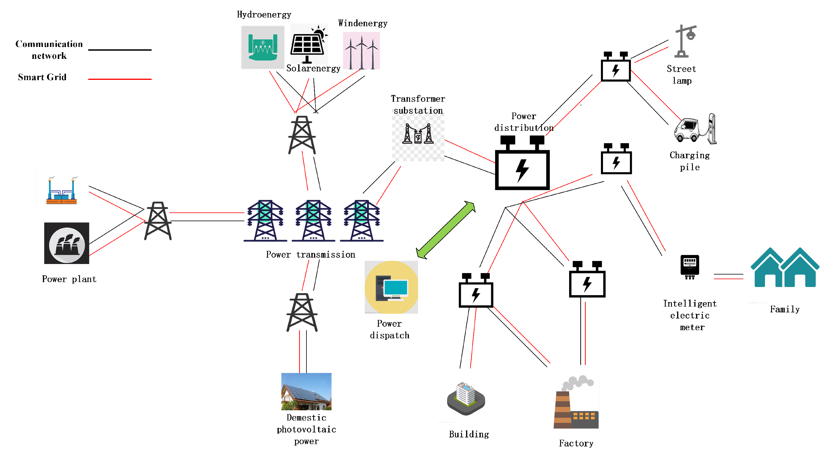
The big data from both the smart grid and the power communication network should be heterogeneous and multidimensional due to the different kinds of sensors. The big data should also be sparse, and some key elements are missing due to unideal operation scenarios.

The DF scheme is shown in Figure 2, where the big data generated from both networks are completed and decomposed with tensor completion and tensor decomposition.

The big data is first transformed into the tensor format, meaning that the sparse and heterogeneous data are compacted into a given tensor format, such as $\mathcal{S}$ and $\mathcal{C}$. The tensor completion is used to complete the missing elements of $\mathcal{S}$ and $\mathcal{C}$. The tensor decomposition is used to analyze the tensor big data from a specific dimension, such as time, frequency, or value. The tensor big data from both networks $\mathcal{S}$ and $\mathcal{C}$ are provided to the fusion function $\mathrm{F}(\mathcal{S},\mathcal{C})$ as indicated in (1) and the fused tensor data $\mathcal{D}$ is generated with the given format.

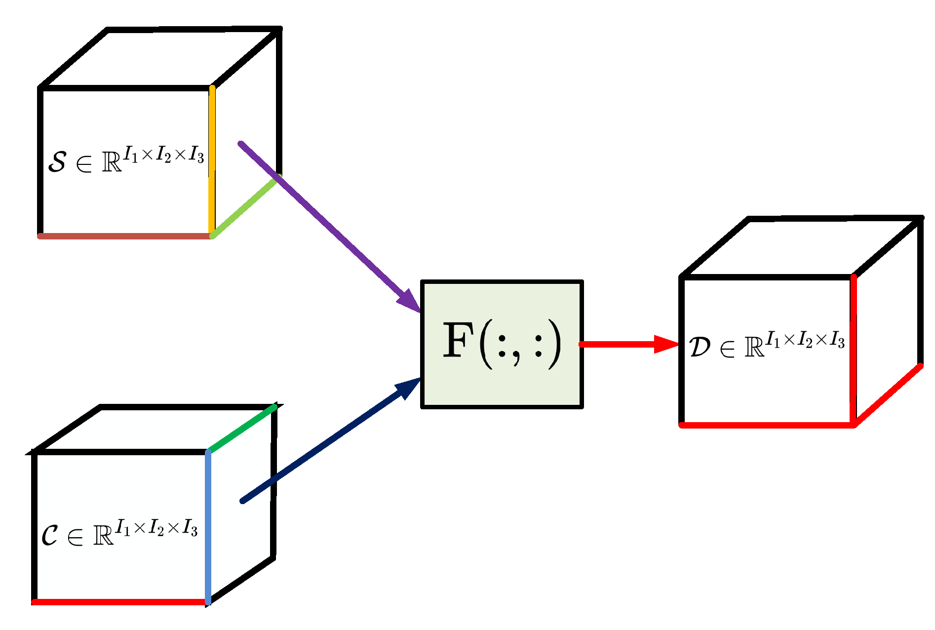
The data fusion scheme is shown in Figure 3, where both the tensor data $\mathcal{S}$ of the smart grid and the tensor data $\mathcal{C}$ of the power communication network are assumed to be the third-order tensors, i.e., $\mathcal{S}\in {\mathbb{R}}^{I_1\times I_2\times I_3}$ and $\mathcal{C}\in {\mathbb{R}}^{I_1\times I_2\times I_3}$. Three dimensions $I_1,I_2$, and $I_3$ can present different dimensions, such as the time T, the frequency F, and the value V. The heterogeneous and multidimensional big data from both networks can be compacted and denoted by sparse tensors. With this expression method, the big data can be processed in an efficient and low-complexity way. The key function of DF is $\mathrm{F}(\mathcal{S},\mathcal{C})$, which generates a new tensor data $\mathcal{D}$ with the same tensor format $\mathcal{D}\in {\mathbb{R}}^{I_1\times I_2\times I_3}$. The fused tensor data $\mathcal{D}$ is used to indicate the total states of two networks, and two networks can also be analyzed based on $\mathcal{D}$. Based on the fused tensor data $\mathcal{D}$, the situation of both networks can be sensed and evaluated.

4. Situation Awareness Based on Deep Reinforcement Learning

DF scheme provides an efficient way to process and express the big data from both networks based on tensor computing. Tensor completion and decomposition schemes also provide solutions to deal with sparse tensor big data and analyze them from a specific dimension. The fused tensor big data can be used in SA. Some key information can be analyzed and generated from the fused tensor data $\mathcal{D}$.

4.1. Situation State and Observation State

The situation state can be modeled and compacted in tensor data $\mathcal{D}$, in which multidimensional elements are used to indicate the situations of two networks. For example, the key information of the smart grid can be presented with tensor data $\mathcal{S}$. The operation information, such as current, total consumption, and so on, can be compacted into the tensor data. Moreover, the key information of the power communication network, such as bandwidth, outage probability, data rate, spectrum efficiency, and so on, can be compacted into tensor data $\mathcal{C}$.

The situation state can be sensed by N agents from K channels, so the state information in the time slot t by the nth agent can be expressed as a K-length state vector ${\mathbf{s}}_n^t=\left\{s_{n1}^t,\dots ,s_{nk}^t,\dots ,s_{nK}^t\right\}$, where $s_{nk}^t\in \left\{0,1\right\}$ denotes two working states: correct (1) or wrong (0). The state values 1 and 0 are used to indicate whether the situation state is correct, meaning that the current state is working well. With N agents, for a given time slot t, a $N\times K$ situation state matrix ${\mathbf{S}}^t$ can be generated. For a period time T, a $N\times K\times T$ state tensor $\mathcal{S}\in {\mathbb{R}}^{N\times K\times T}$ can be formulated. Note that the state matrix ${\mathbf{S}}^t$ can be calculated by the state tensor $\mathcal{S}$ from a specific dimension. Therefore, based on tensor big data $\mathcal{S}$ and $\mathcal{C}$, the situation states of both networks can be formulated in the format of tensors. Following the same way, the observation state of the nth agent in the time slot t can be expressed as a K-length observation vector ${\mathbf{o}}_n^t=\left\{o_{n,1}^t,\dots ,o_{n,k}^t,\dots ,o_{n,K}^t\right\}$, where $o_{nk}^t\in \{0,1\}$. The $N\times K\times T$ observation tensor $\mathcal{O}\in {\mathbb{R}}^{N\times K\times T}$ can be generated.

4.1.1. Agent Action

Total N agents are used to sense the situation states with K channels in total T time slots. The action of the agent is used to sense the current state and return sense results. The action of N agents can be defined as ${\mathbf{A}}^t=\left\{{\mathit{a}}_1^t,\dots ,{\mathit{a}}_n^t,\dots ,{\mathit{a}}_N^t\right\}$, where ${\mathit{a}}_n^t$ denotes a K-length action vector and the element $a_{n,k}^t\in \{0,1\}$ means the n-th agent takes the action at the k-th channel at the t-th time slot. The action of 1 indicates that the result of action (sensing) is correct with the current real situation.

4.1.2. System Reward

When the n-th agent senses the current situation state successfully, the system can receive reward feedback denoted by a given number. Define the N-length agent reward vector as ${\mathit{r}}^t=\left\{r_1^t,\dots ,r_n^t,\dots ,r_N^t\right\}$ and let $r_n^t$ denote the reward for the n-th agent at the t-th time slot. When the agent can sense the situation state correctly, a positive reward $\overline{r}$ is returned to the system; otherwise, a negative reward p as a penalty will be returned. The reward $r_n^t$ of the n-th agent at the t-th time slot can be given as

$$r_n^t=\left\{\begin{array}{cc}{\overline{r}}_n,\hfill & \mathrm{Correct}\mathrm{results}\hfill \\ {\overline{r}}_n+p_n,\hfill & \mathrm{Without}\mathrm{results}\hfill \\ p_n,\hfill & \mathrm{Wrong}\mathrm{results}\hfill \end{array}\right.$$

(13)

where ${\overline{r}}_n$ and $p_n$ are used to denote the positive and negative rewards, respectively.

For the proposed SA scheme, the final goal is to achieve an optimal sensing strategy ß to train the whole system to obtain the maximum reward, in other words, all N agents should work together to obtain situation states correctly. So we define a long-term accumulated reward $J_{\pi }$, which is based on the given policy $\pi$. The accumulated reward $J_{\pi }$ based on the reward function can be expressed as

$$J_{\pi }=\mathbb{E}\left(\sum _{t=0}^T{\gamma }^t{r}_n^t\right)$$

(14)

where $\mathbb{E}(·)$ is the expectation function, $\gamma \in [0,1]$ is denotes a loss factor and $t\in [1,T]$ is the time cumulative series.

4.2. Deep Reinforcement Learning Scheme

In order to achieve an optimal SA scheme, the DQN algorithm and the MAAC algorithm are discussed.

4.2.1. Deep Q-Network Algorithm

The DQN algorithm is currently one of the most popular reinforcement learning algorithms. It can be used in dynamic situation environment, and huge state spaces. Each agent has an independent DQN network, where the input is the observation state and the output is the corresponding Q value. Then the network is updated and iterated with the following formulation

$$\begin{array}{cc}\hfill Q({\mathit{s}}_n^t,{\mathit{a}}_n^t)& \leftarrow Q({\mathit{s}}_n^t,{\mathit{a}}_n^t)+\beta [r_n^t+\gamma \underset{{\mathit{a}}_n^{t+1}}{max}\widehat{Q}({\mathit{s}}_n^{t+1},{\mathit{a}}_n^{t+1})-Q({\mathit{s}}_n^t,{\mathit{a}}_n^t)]\hfill \end{array}$$

(15)

where $\widehat{Q}\left({\mathit{s}}_n^{t+1},{\mathit{s}}_n^{t+1}\right)$ is the output Q value of the target network, $\beta \in [0,1]$ is the learning rate. The action selection policy in DQN adopts the $ϵ$-greedy policy to find the optimal policy ${\pi }_n^{*}$, which can be expressed as

$${\pi }_n^{*}=\underset{{\mathit{a}}_n^t}{argmax}Q({\mathit{s}}_n^t,{\mathit{a}}_n^t)$$

(16)

where ${\pi }_n^{*}$ denotes the optimal policy of the n-th agent.

4.2.2. MAAC Algorithm

Each agent can perform a dynamic SA scheme based on the MAAC algorithm [21]. There are total N agents, which can simultaneously sense the situation and perform the corresponding actions to obtain system rewards. The system is distributed, and each agent should select actions independently using training networks. Additionally, each agent has an actor network to take action and a critic network to evaluate its actions. Using N agents, the system can sense the situation and take the corresponding actions. In order to achieve the optimal policy for the system, all agents should learn the way to sense the situation, take action and obtain rewards. All agents receive their rewards and evaluate their actions by those rewards.

The parameters of the actor network and the critic network are $\varphi$ and $\theta$, respectively. In the actor network, the observed state ${\mathit{s}}_n^t$ of the agents is the input, and the action ${\mathit{a}}_n^t$ is the output. The action selection function selects the action ${\mathit{a}}_n^t$ based on the policy ${\pi }_n^{\varphi }$ and the process can be described as ${\pi }_n^{\varphi }\left({\mathit{s}}_n^t\right)$. In the critic network, the current action ${\mathit{a}}_n^t$ obtained from the actor network and the current observation state ${\mathit{s}}_n^t$ are input, the Q-value $Q^{\theta }({\mathit{s}}_n^t,{\mathit{a}}_n^t)$ is output, which is used to evaluate the actions. For each agent, the actor network is used to sense the situation and take the corresponding actions, and the critic network is used to evaluate its action based on the given policy.

The n-th agent senses the situation, obtains the rewards, and calculates the Q-value $Q^{\theta }({\mathit{s}}_n^t,{\mathit{a}}_n^t)$ with the critic and the target critic networks. In this case, the loss function can be defined to update the critic network. The loss function ${\mathcal{L}}_n\left(\theta \right)$ of the n-th agent for the parameter $\theta$ can be formulated as

$${\mathcal{L}}_n\left(\theta \right)={\mathbb{E}}_{({\mathit{s}}_n^t,{\mathit{a}}_n^t,r_n^t,{\mathit{s}}_n^{t+1})\sim D}[\left(Q^{\theta }({\mathit{s}}_n^t,{\mathit{a}}_n^t)-Z_n^{t+1}{)}^2\right],$$

(17)

where D is the replay buffer and the function $Z_n$ can be defined as

$$\begin{array}{cc}\hfill Z_n^{t+1}=r_n^t+\gamma {\mathbb{E}}_{{\mathit{a}}_n^{t+1}\sim {\pi }_n^{\widehat{\varphi }}\left({\mathit{s}}_n^{t+1}\right)}[& Q^{\widehat{\theta }}({\mathit{s}}_n^{t+1},{\mathit{a}}_n^{t+1})+e({\mathit{s}}_n^{t+1},{\mathit{a}}_n^{t+1})].\hfill \end{array}$$

(18)

For the actor network and the critic network, the parameters are $\widehat{\varphi }$ and $\widehat{\theta }$, respectively. Two parameters of the target networks can be updated by

$$\begin{array}{c}\widehat{\varphi }\leftarrow \tau \varphi +(1-\tau )\widehat{\varphi },\hfill \\ \widehat{\theta }\leftarrow \tau \theta +(1-\tau )\widehat{\theta }\hfill \end{array}$$

(19)

where the parameter $\tau \in [0,1]$ is a soft update factor. The proposed MAAC algorithm for SA is summarized in Algorithm 3.

Algorithm 3 The MAAC Algorithm for SA

Initialization:  Randomly initialize network parameters $\varphi , \widehat{\varphi }, \theta , \mathrm{and} \widehat{\theta }$.  Initialize buffer O.  Simultaneously obtain initial observation states S0 for all agents with sensing accuracy μ. 1: for $t=0,1,2,\dots$ do 2:     for $n=1,\dots ,N$ do 3:         Each agent sequentially and independently selects the action ${\mathit{A}}_n^t$ based on the policy ${\pi }_n^{\varphi }\left({\mathit{S}}_n^t\right)$. 4:     end for 5:     Simultaneously execute actions ${\mathit{A}}^t$ for all agents to obtain rewards ${\mathit{R}}^t$. 6:     Update environment to obtain new observation states ${\mathit{S}}^{t+1}$. 7:     Store replay units $({\mathit{S}}^t,{\mathit{A}}^t,{\mathit{R}}^t,{\mathit{S}}^{t+1})$ of all agents in O. 8:     for $n=1,\dots ,N$ do 9:         Randomly sample a mini-batch of replay units $({\mathit{S}}_n^t,{\mathit{A}}_n^t,R_n^t,{\mathit{S}}_n^{t+1})$ from O. 10:         Calculate Q-value $Q^{\theta }({\mathit{S}}_n^t,{\mathit{A}}_n^t)$ by the critic network. 11:         Calculate ${\mathit{A}}_n^{t+1}\sim {\pi }_n^{\widehat{\varphi }}\left({\mathit{S}}_n^{t+1}\right)$ and $Q^{\widehat{\theta }}({\mathit{S}}_n^{t+1},{\mathit{A}}_n^{t+1})$ by target actor network and target       critic network, respectively. 12:         Calculate regression loss function ${\mathcal{L}}_n\left(\theta \right)$ to update the critic network. 13:         Calculate ${\mathit{A}}_n^t\sim {\pi }_n^{\varphi }\left({\mathit{S}}_n^t\right)$ via the actor network and $Q^{\theta }({\mathit{S}}_n^t,{\mathit{A}}_n^t)$ via the critic network. 14:         Update the action network by computing the policy gradient ${\nabla }_{\varphi }J\left({\pi }_n\right)$. 15:         Soft update parameters of target networks by (19). 16:     end for 17: end for

5. Simulation Results

In this section, the proposed DF and SA are evaluated and analyzed by simulations. Two kinds of simulations are provided to evaluate the proposed tensor-based DF scheme and DRL-based SA scheme.

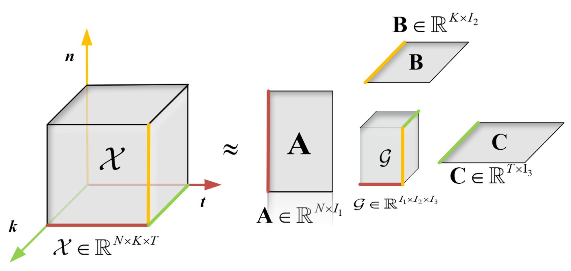
In Figure 4, a third-order tensor $\mathcal{X}\in {\mathbb{R}}^{N\times K\times T},(N=K=T=3)$ is used to illustrate the process of tensor decomposition. The tensor $\mathcal{X}$ is decomposed into one core tensor $\mathcal{G}\in {\mathbb{R}}^{I_1\times I_3\times I_3}$ and three matrices $\mathbf{A}\in {\mathbb{R}}^{N\times I_1}$, $\mathbf{B}\in {\mathbb{R}}^{K\times I_2}$, and $\mathbf{C}\in {\mathbb{R}}^{T\times I_3}$.

Therefore, the tensor decomposition scheme provides a way to analyze the tensor big data of smart grid and power communication networks, such as $\mathcal{S}$ and $\mathcal{C}$. The core tensor $\mathcal{G}$ can be used to keep the core information with the reduced dimensions $I_1\times I_3\times I_3$ and the three matrices $\mathbf{A}$, $\mathbf{B}$, and $\mathbf{C}$ can be used to denote the information for the given dimension.

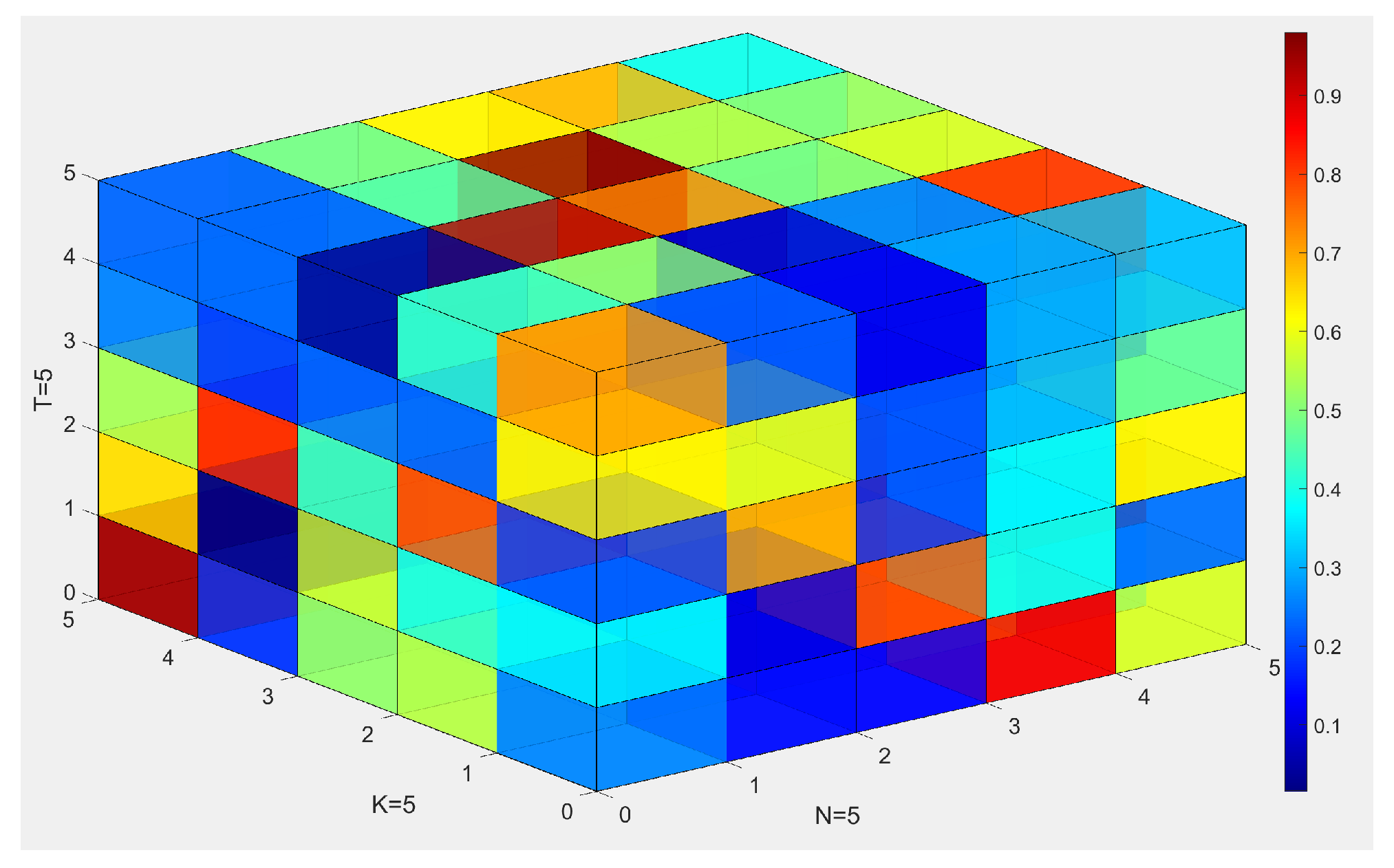
The fused tensor $\mathcal{D}\in {\mathbb{R}}^{N\times K\times T},(N=K=T=5)$ is shown in Figure 5, where there are total 125 elements ${\mathcal{D}}_{n,k,t},n\in [1,5],k\in [1,5],t\in [1,5]$ in the tensor big data. As indicated by the color bar, the value of the element is normalized by one unit. Different colors are used to indicate different element values. As indicated in this figure, the fused tensor $\mathcal{D}$ is generated from the tensor big data $\mathcal{S}$ and $\mathcal{C}$ as shown in Figure 3. The fused tensor $\mathcal{D}$ can also be analyzed from three dimensions: five agents $N=5$, five channels $K=5$, and five time slots $T=5$. For a specific location, say ${\mathcal{D}}_{1,1,1}$, the fused data can be evaluated by the value $|{\mathcal{D}}_{1,1,1}|$.

By comparing the simulation results of the MAAC algorithm and the DQN algorithm, we evaluate the performance of the MAAC algorithm. In our simulations, for both algorithms, we set the episodes as 120,000, the reward of successful allocation r as 10, the reward of no allocation negative f as −5, and the batch size as 128, which is the number of parameters transmitted to the program for training at a time. The discount factor $\gamma$ of the MAAC algorithm is set as 0.9, the exploration rate $ϵ$ of the DQN algorithm decreases from 0.9 to 0.

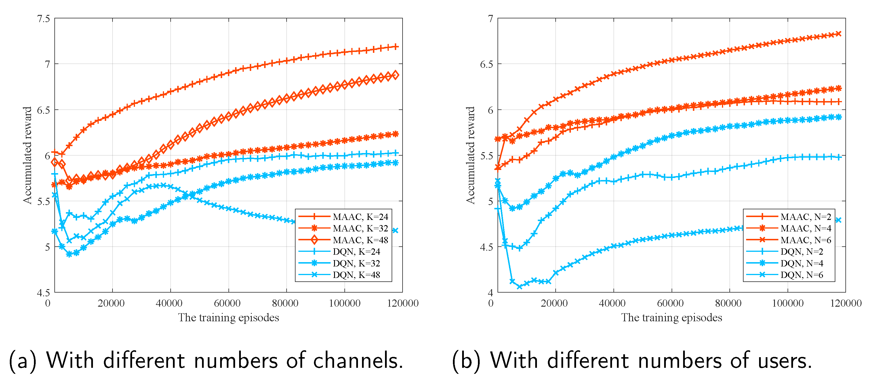
We compare the performances of the DQN algorithm and the MAAC algorithm when the number of channels is different; N = 4, and the sensing probability p = 0.9, the accumulated reward of the system is the average reward of all agents during previous episodes.

It can be seen in Figure 6a, when K = 24, K = 32, and K = 48, the accumulated reward of the DQN algorithm increases when the training episodes = 120,000, while the accumulated reward of the MAAC algorithm is significantly higher than the reward of the DQN algorithm, the accumulated reward of the MAAC algorithm is higher than that of the DQN algorithm, and the training process of the MAAC algorithm is more stable than that of the DQN algorithm.

Then we compare the performance of the DQN algorithm and the MAAC algorithm with the different number of agents when the sensing probability p = 0.8 and the number of channels K = 32.

As shown in Figure 6b, the MAAC algorithm not only accumulated a higher reward than the DQN algorithm but also the convergence speed is faster than the DQN algorithm; when N = 2, N = 4, and N = 6, the convergence of the MAAC algorithm is earlier than that of the DQN algorithm.

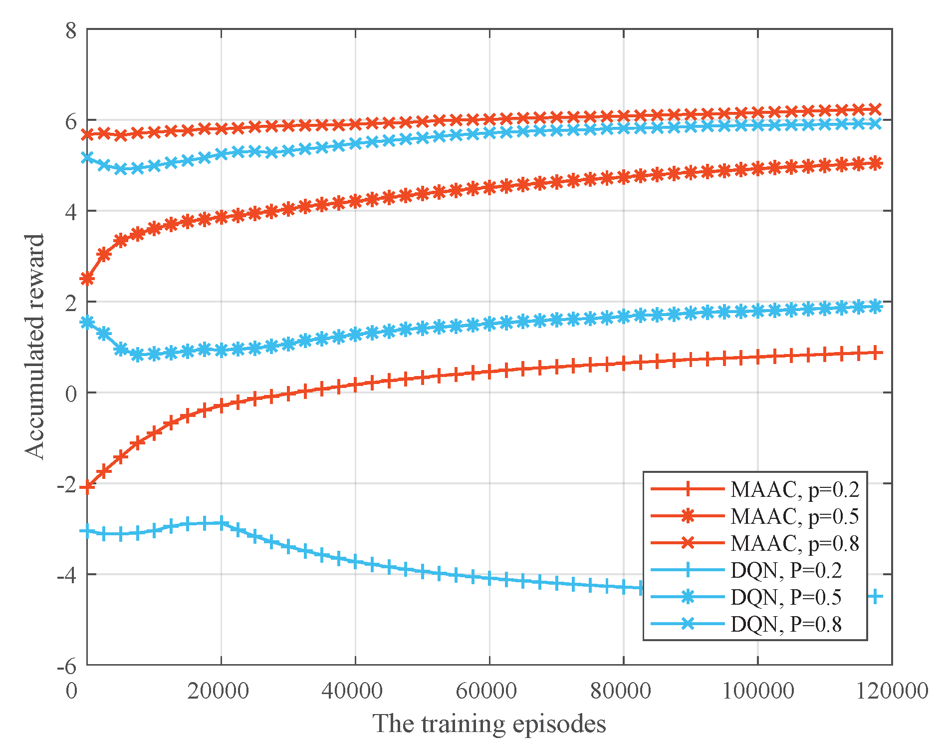
In Figure 7, we compare the performances of the DQN algorithm and MAAC algorithm under different sensing probabilities. With the same parameters, the accumulated reward of the MAAC algorithm is always higher than the DQN algorithm. For the two algorithms, the higher the sensing probability, the higher the accumulated reward; when the sensing probability is very high such as p = 0.8, the rewards of the two algorithms tend to be approximate.

6. Conclusions

In this paper, the data fusion and situation awareness problems for the smart grid and the power communication network have been studied using tensor computing and deep reinforcement learning. For heterogeneous and multidimensional big data from two networks, we involved tensor computing in modeling those big data and used tensor completion/decomposition schemes to analyze tensor format big data. For the tensor big data, we used deep reinforcement learning to train multiple-agent networks to learn the optimal situation sensing scheme to sense the situation state. A novel MAAC algorithm has been proposed to achieve the optimal sensing scheme, in which the actor network and the critic network have been used by each agent to independently train and learn the optimal sensing policy. Simulation results have demonstrated that the tensor-based data presentation scheme provides an efficient way to present the big data from two networks. Moreover, the proposed MAAC algorithm can achieve better performance compared with the conventional DQN scheme. This paper has provided practical guidance to deal with big data from data fusion and situational awareness for the smart grid and the power communication network.

References

1. Xi, L.; Wang, Y.; Wang, Y.; Wang, Z.; Wang, X.; Chen, Y. Deep Reinforcement Learning-Based Service-Oriented Resource Allocation in Smart Grids. IEEE Access 2021, 9, 77637–77648. [Google Scholar] [CrossRef]
2. Kong, W.; Dong, Z.Y.; Jia, Y.; Hill, D.J.; Xu, Y.; Zhang, Y. Short-Term Residential Load Forecasting Based on LSTM Recurrent Neural Network. IEEE Trans. Smart Grid 2019, 10, 841–851. [Google Scholar] [CrossRef]
3. Tushar, W.; Saha, T.K.; Yuen, C.; Smith, D.; Poor, H.V. Peer-to-Peer Trading in Electricity Networks: An Overview. IEEE Trans. Smart Grid 2020, 11, 3185–3200. [Google Scholar] [CrossRef] [Green Version]
4. Cosovic, M.; Tsitsimelis, A.; Vukobratovic, D.; Matamoros, J.; Anton-Haro, C. 5G Mobile Cellular Networks: Enabling Distributed State Estimation for Smart Grids. IEEE Commun. Mag. 2017, 55, 62–69. [Google Scholar] [CrossRef] [Green Version]
5. Zerihun, T.A.; Garau, M.; Helvik, B.E. Effect of Communication Failures on State Estimation of 5G-Enabled Smart Grid. IEEE Access 2020, 8, 112642–112658. [Google Scholar] [CrossRef]
6. Xu, W.; Chen, W.; Fan, Y.; Zhang, Z.; Shi, X. Spectrum efficiency maximization for cooperative power beacon-enabled wireless powered communication networks. China Commun. 2021, 18, 230–251. [Google Scholar] [CrossRef]
7. Min, Z.; Muqing, W.; Lilin, Q.; Quanbiao, A.; Sixu, L. Evaluation of Cross-Layer Network Vulnerability of Power Communication Network Based on Multi-Dimensional and Multi-Layer Node Importance Analysis. IEEE Access 2022, 10, 67181–67197. [Google Scholar] [CrossRef]
8. Tang, X.; Cao, C.; Wang, Y.; Zhang, S.; Liu, Y.; Li, M.; He, T. Computing power network: The architecture of convergence of computing and networking towards 6G requirement. China Commun. 2021, 18, 175–185. [Google Scholar] [CrossRef]
9. Li, Y.; Zhang, M.; Zhu, W.; Cheng, M.; Zhou, C.; Wu, Y. Performance evaluation for medium voltage MIMO-OFDM power line communication system. China Commun. 2020, 17, 151–162. [Google Scholar] [CrossRef]
10. He, X.; Qiu, R.C.; Ai, Q.; Chu, L.; Xu, X.; Ling, Z. Designing for Situation Awareness of Future Power Grids: An Indicator System Based on Linear Eigenvalue Statistics of Large Random Matrices. IEEE Access 2016, 4, 3557–3568. [Google Scholar] [CrossRef]
11. Li, Q.; Tang, H.; Liu, Z.; Li, J.; Xu, X.; Sun, W. Optimal Resource Allocation of 5G Machine-Type Communications for Situation Awareness in Active Distribution Networks. IEEE Syst. J. 2022, 16, 4187–4197. [Google Scholar] [CrossRef]
12. Wu, J.; Ota, K.; Dong, M.; Li, J.; Wang, H. Big Data Analysis-Based Security Situational Awareness for Smart Grid. IEEE Trans. Big Data 2018, 4, 408–417. [Google Scholar] [CrossRef] [Green Version]
13. Wang, P.; Govindarasu, M. Multi-Agent Based Attack-Resilient System Integrity Protection for Smart Grid. IEEE Trans. Smart Grid 2020, 11, 3447–3456. [Google Scholar] [CrossRef]
14. He, X.; Ai, Q.; Qiu, R.C.; Huang, W.; Piao, L.; Liu, H. A Big Data Architecture Design for Smart Grids Based on Random Matrix Theory. IEEE Trans. Smart Grid 2017, 8, 674–686. [Google Scholar] [CrossRef] [Green Version]
15. Zhang, W.; Wu, J.; Wang, C.X. Tensor-computing-based Spectrum Usage Framework for 6G. In Proceedings of the ICC 2020–2020 IEEE International Conference on Communications (ICC), Dublin, Ireland, 7–11 June 2020; pp. 1–6. [Google Scholar] [CrossRef]
16. Kolda, T.G.; Bader, B.W. Tensor decompositions and applications. Siam Rev. 2009, 51, 455–500. [Google Scholar] [CrossRef]
17. Sidiropoulos, N.D.; De Lathauwer, L.; Fu, X.; Huang, K.; Papalexakis, E.E.; Faloutsos, C. Tensor decomposition for signal processing and machine learning. IEEE Trans. Signal Process. 2017, 65, 3551–3582. [Google Scholar] [CrossRef]
18. Liu, J.; Musialski, P.; Wonka, P.; Ye, J. Tensor completion for estimating missing values in visual data. IEEE Trans. Pattern Anal. Mach. Intell. 2012, 35, 208–220. [Google Scholar] [CrossRef] [PubMed]
19. Yokota, T.; Zhao, Q.; Cichocki, A. Smooth PARAFAC decomposition for tensor completion. IEEE Trans. Signal Process. 2016, 64, 5423–5436. [Google Scholar] [CrossRef] [Green Version]
20. Li, Y.; Zhang, W.; Wang, C.X.; Sun, J.; Liu, Y. Deep Reinforcement Learning for Dynamic Spectrum Sensing and Aggregation in Multi-Channel Wireless Networks. IEEE Trans. Cogn. Commun. Netw. 2020, 6, 464–475. [Google Scholar] [CrossRef]
21. Ding, W.; Zhang, W.; Wang, D.; Sun, J.; Wang, C.X. Dynamic Spectrum Aggregation and Access Scheme Based on Multi-Agent Actor-Critic Reinforcement Learning. In Proceedings of the 2021 13th International Conference on Wireless Communications and Signal Processing (WCSP), Changsha, China, 20–22 October 2021; pp. 1–5. [Google Scholar] [CrossRef]
Figure 1. Smart grid with power communication network based on 5G systems.
Electronics 12 02606 g001
Figure 2. Data fusion flow diagram.
Electronics 12 02606 g002
Figure 3. Tensor based data fusion sketch.
Electronics 12 02606 g003
Figure 4. Tensor decomposition for situation tensor X .
Electronics 12 02606 g004
Figure 5. Fused tensor D .
Electronics 12 02606 g005
Figure 6. Accumulated reward of two algorithms with different parameters.
Electronics 12 02606 g006
Figure 7. Accumulated reward of two algorithms with different sensing probabilities.
Electronics 12 02606 g007
Disclaimer/Publisher’s Note: The statements, opinions and data contained in all publications are solely those of the individual author(s) and contributor(s) and not of MDPI and/or the editor(s). MDPI and/or the editor(s) disclaim responsibility for any injury to people or property resulting from any ideas, methods, instructions or products referred to in the content.