A Complex Empirical Mode Decomposition for Multivariant Traffic Time Series

Abstract

Data-driven modeling methods have been widely used in many applications or studies of traffic systems with complexity and chaos. The empirical mode decomposition (EMD) family provides a lightweight analytical method for non-stationary and non-linear data. However, a large amount of traffic data in practice are usually multidimensional, so the EMD family cannot be used directly for those data. In this paper, a method to calculate the extremum point and the envelope-like function (series) from the complex function (series) is proposed so that the EMD family can be applied to two-variate traffic time-series data. Compared to the existing multivariate EMD, the proposed method has advantages in computational burden, flexibility and adaptivity. Two-dimensional trajectory data were used to test the method and its oscillatory characteristics were extracted. The decomposed feature can be used for data-driven traffic analysis and modeling. The proposed method also extends the utilization of EMD to multivariate traffic data for applications such as traffic data denoising, pattern recognition, traffic flow dynamic evaluation, traffic prediction, etc.

1. Introduction

Because of the complexity and chaos of traffic systems, it is hard to investigate the system state estimates or mode identification via the method of directly modeling. Thus, data-driven modeling methods have been widely used in many applications or studies concerning intelligent traffic, and the research regarding digital traffic has become a branch of intelligent traffic, which includes traffic feature analysis, traffic flow estimate, bus arrival estimate, traffic jam identification, traffic events and accident analysis. On the other hand, the development of artificial intelligence empowers intelligent traffic and brings huge benefits. As one of the three key elements of artificial intelligence, data play an important role in applications and research.

A large number of studies of traffic modeling via time series have taken place. Chin and Quddus [1] use the random-effect negative binomial (RENB) model to investigate the elements appropriate for maintaining safety in road intersections. Brijs, Karlis and Wets [2] and Quddus [3] used integer-valued autoregressive Poisson models to model data of accidents and investigate the relation of accidents and some specific factors. Commandeur, Bijleveld, Bergel-Hayat et al. [4] and Saar [5] used auto-regression and moving average model to investigate the correlation of traffic accidents and some other factors. For panel data analysis, F. Chen, Ma and S. Chen [6,7] introduced random-effect tobit models to investigate the relationship between traffic crashes and several factors such as traffic states, weather and surface conditions. Later, methods such as full Bayesian hierarchical approach and multivariate Poisson lognormal models were used to investigate traffic crash modeling and factors regarding traffic accidents [8,9,10]. In recent years, while regression models have still been widely used as the foundation of time series data analysis, some machine learning methods have been introduced to improve the performance. Tuli, Mitra and Crews [11] employed a random-effect negative binomial (RENB) model to investigate the demand for shared bicycles. Barroso, Albuquerque-Oliveira and Oliveira-Neto [12] introduced clustering methods to define traffic profiles and the daily traffic periods in trip analyses based on OD data. Chang, Huang, Chan et al. [13] introduced long-memory properties to investigate road fatality factors.

Traffic time series data contain multiple mode characteristics, so mode decomposition of such data is essential for better analysis and modeling. Commonly used modal decomposition methods for time-series data include discrete wavelet transform (DWT), empirical mode decomposition (EMD) and variational mode decomposition (VMD). EMD, in particular, allows for adaptive decomposition of data and efficient handling of nonlinear and non-smooth data without significant computational burden. EMD has been utilized in many traffic and transportation applications such as traffic data denoising [14,15], traffic infrastructure healthy monitoring [16], traffic flow evolving dynamic evaluation [17] and time variant detection [18], as well as prediction of section traffic flow [19], traffic speed [20] and metro passenger flow [21]. However, current empirical mode decomposition methods such as EMD, EEMD, CEEMD and CEEMDAN are not equipped to handle multivariate data directly. Since the traffic system generates many multivariate time series data, such as trajectory data, there is a pressing need to extend classical empirical mode decomposition methods to deal with multivariate time series.

In this paper, a complex empirical mode decomposition operation was proposed to extract intrinsic mode functions from multivariate traffic time series data. It provides a tool to analyze multivariate temporal data which extends the application of intrinsic mode extraction on multivariate traffic data. Complex extremum-like point and complex envelope-like series were defined by introducing the “base angle” for sifting through the intrinsic mode function. The proposed method avoided large computational burdens and appeared to be more flexible and adaptive. The experiment showed that the proposed method is able to extract oscillation mode and motion characteristics of moving trajectory. Existing multivariant empirical mode decomposition methods are reviewed in Section 2. The proposed complex empirical mode decomposition method is introduced in Section 3. The trace mode decomposition is presented in Section 4. The conclusion is presented in Section 5.

2. Related Work

Original empirical mode decomposition [22] provides a method to extract intrinsic mode functions from non-stationary time series signals. The conditions which the IMF satisfies and the procedures to extract IMFs are closely related to the extremum and envelope function. However, for multi-dimension signals, common extremum and envelope functions do not exist. So, the original EMD cannot be applied directory to multi-dimension signals.

Several researchers have proposed decomposition methods for complex-valued data. Tanka and Mandic [23] decomposed complex-valued data into positive frequency components and negative frequency components. A band-pass filter was used so that both positive and negative frequency components are analytic signals, which means the real part of those components contains complete information of the original signal. Then the classical EMD was used to extract IMFs. This method made clever use of the band-pass filter and the characteristic of analytic signal, but the two sets of IMFs from positive and negative components cannot be linked intuitively to the original signal.

Another idea is to extend the definition of the envelope function or extremum point. Bin Altaf, Gautama, Tanaka et al. [24] proposed a new definition of extremum of complex-valued data series in which the extremum points were found according to whether the first derivative changes its sign. Then the complex-valued envelope functions and the average can be computed. This method decomposes the complex-valued signal directory without separating the signal into two parts so that the results are more intuitive. Rilling, Flandrin, Goncalves et al. [25] extend the “oscillation” in two dimensions to the “rotation” in three dimensions so the task is to decompose the rotation modes, such as “rapid” and “slower” rotation, of complex-valued signals (data series). The extremum points were defined as the tangent points to the top, bottom, left and right. Those points were linked by a cubic spline to be the envelope functions. This method, from the perspective of subsequent studies, uses a fixed projection to calculate the extrema points and the envelope which may miss the combined effect of multiple variables.

Rehman and Mandic [26] proposed an extension of EMD for trivariate signals in which projection directions were introduced to find the extrema points and calculate envelope curves. To choose those directions, a sphere in signal space was built and multiple longitudinal lines were uniformly chosen on that sphere. Then a series of equidistant points on each longitudinal line was taken as the projection directions. Along those projection directions, maximum points of the input signal were found and the envelope curves was obtained by interpolating those maximum points (along each direction). After that, the two authors proposed an advanced method for n-variate signals in which the projection directions were chosen more uniformly [27]. For n-variate input, the low-discrepancy pointsets were used to generate uniform points on the n-1 sphere as projection directions. This method was widely used in many subsequent studies. However, the computational effort of this method is very high. Inspired by some studies of non-temporal multidimensional empirical mode decomposition. Thirumalaisamy and Ansell [28] proposed a fast and adaptive multivariate EMD method in which order statistics filter was used to take the place of classical spline interpretation so that the computational cost could be reduced and Delaunay triangulation and sparable filters were used to reduce the computational cost of projection calculation. However, even though the method proposed was an improvement, the algorithm of the Multivariate EMD was still a bit complicated.

Fleureau, Kachenoura, Albera et al. [29,30] proposed a method to obtain a signal’s mean trend by interpolating barycenter which was computed from identified elementary oscillations. A D+1 dimension tangent vector of a D dimension signal was defined. The oscillation extremum defined in this method was the point where the norm of the “tangent” reaches the local minimum. Then, rather than calculating envelope curves to obtain the mean curve, the concept oscillation barycenter was introduced to calculate the mean curve directly. An oscillation barycenter was defined to be a point between two oscillation extremum points. The time coordination of one barycenter point was set to the intermediate moment of its adjacent two extreme points. The variate values of the barycenter were defined to be the average of the signal variate integrals between the two extreme points. The authors improved this method later by changing the calculation of the mean curve [31]. The envelope curves were reintroduced to calculate the mean curve. The even oscillation extremum and odd oscillation extremum were interpolated separately to obtain two envelope curves. This method extended the original EMD to a multidimensional signal. However, the extremum identification algorithm may obtain false extremum points from discrete time series, for the differences of the signals are not continuous. For example, a one-dimension signal [0.1, 0.5, 0.7, 0.9, 0.7, 0.1] has minimum norm of “tangent” at the third and fourth points but the fourth point is the extremum point.

3. The Complex Empirical Mode Decomposition

3.1. The Complex Time Series

Original EMD deals with one-dimensional signals. However, in practice, multi-dimensional signals are more common, for example, tracks of moving objects. To decompose such a signal, the two-dimensional time series can be transformed into a complex time series.

Let $s_n=\left(x_n,y_n\right)$, for $n=0,1,2,\dots$ be the two-dimensional time series. $z_n=x_n+i{y}_n=r_n{e}^{i{\theta }_n}$ is the complex form of the series, where $r_n=\sqrt{x_n^2+y_n^2}$ and ${\theta }_n=Arg\left(z_n\right)$.

3.2. The Complex Extremum-Like Point

Similar to the original intrinsic mode function, the complex intrinsic mode function has two conditions: (1) The phase difference of two adjacent extremum points should be between $\frac{\pi }{2}$ and $\frac{3\pi }{2}$. (2) At each time, the mean value of the upper envelope function and the lower envelope function should be zero. Let $\Delta \theta$ be the phrase difference, $U\left(t\right)$ be the upper envelope function and $L\left(t\right)$ be the lower envelope function. The conditions could be described as:

$$\left\{\begin{array}{c}\epsilon \left(cos\Delta \theta \right)=0\hfill \\ L\left(t\right)+U\left(t\right)=0\hfill \end{array}\right.$$

(1)

where $\epsilon \left(x\right)$ is the stage function and was set to 1 when $x=0$.

Typical extremum points do not exist in complex functions, nor in upper or lower envelope functions A definition of extremum-like points including maximum-like and minimum-like points, therefore, was proposed.

Let $B_n$ and $E_n$ be the intermediate series For $n=m$,

$$\begin{array}{cc}\hfill B_m& ={\theta }_m+\frac{\pi }{2}\times \left(1-E_m\right)\hfill \end{array}$$

(2)

$$\begin{array}{cc}\hfill E_m& =sign\left[cos\left({\theta }_m-B_{m-1}\right)\right]\hfill \end{array}$$

(3)

where $sign\left(x\right)=\epsilon \left(x\right)-\epsilon \left(-x\right)$ and for $n=-1$, $B_{-1}=0$. Additionally, $\epsilon \left(x\right)$ was also set to 1 where $x=1$.

Let ${\Delta }_n$ be the forward differential of $B_n\times r_n$:

$${\Delta }_n=E_{n+1}\times r_{n+1}-E_n\times r_n$$

(4)

For $n=t$, $z_t$ is a maximum-like point if the conditions

$$\left\{\begin{array}{c}{\Delta }_t\times {\Delta }_{t-1}<0\hfill \\ {\Delta }_t-{\Delta }_{t-1}<0\hfill \end{array}\right.$$

(5)

were satisfied, and is a minimum-like point if the conditions

$$\left\{\begin{array}{c}{\Delta }_t\times {\Delta }_{t-1}<0\hfill \\ {\Delta }_t-{\Delta }_{t-1}>0\hfill \end{array}\right.$$

(6)

were satisfied.

The intermediate series $B_n$ records the base angles of the data series. Suppose each element of the data series in chronological order is on a curved surface in the complex-time coordinate system. The base angles are the positive direction of the surface. The initial base angle was set to be 0. If the difference between the argument of one datum and the base angle corresponding to the previous datum was within $\left[-\frac{\pi }{2},\frac{\pi }{2}\right]$, the base angle corresponding to this datum was set to be the argument of this datum. Otherwise, if  the difference was within $\left[-\pi ,-\frac{\pi }{2}\right)\cup \left(\frac{\pi }{2},\pi \right)$, the base angle was set to be the argument plus $\pi$. If the curved surface was flattened into a plane, the condition to find the extremum-like point is the same as the condition to determine the maximum and minimum points in real series.

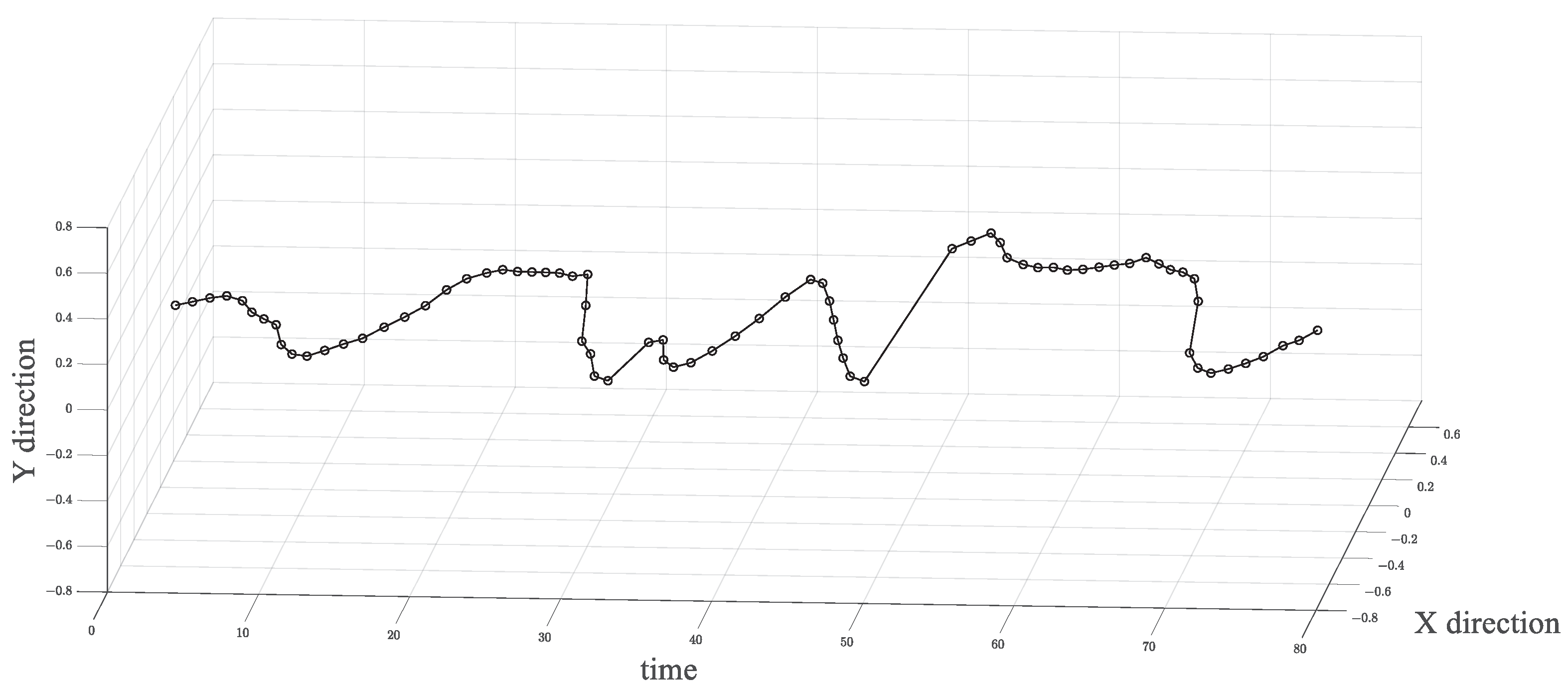
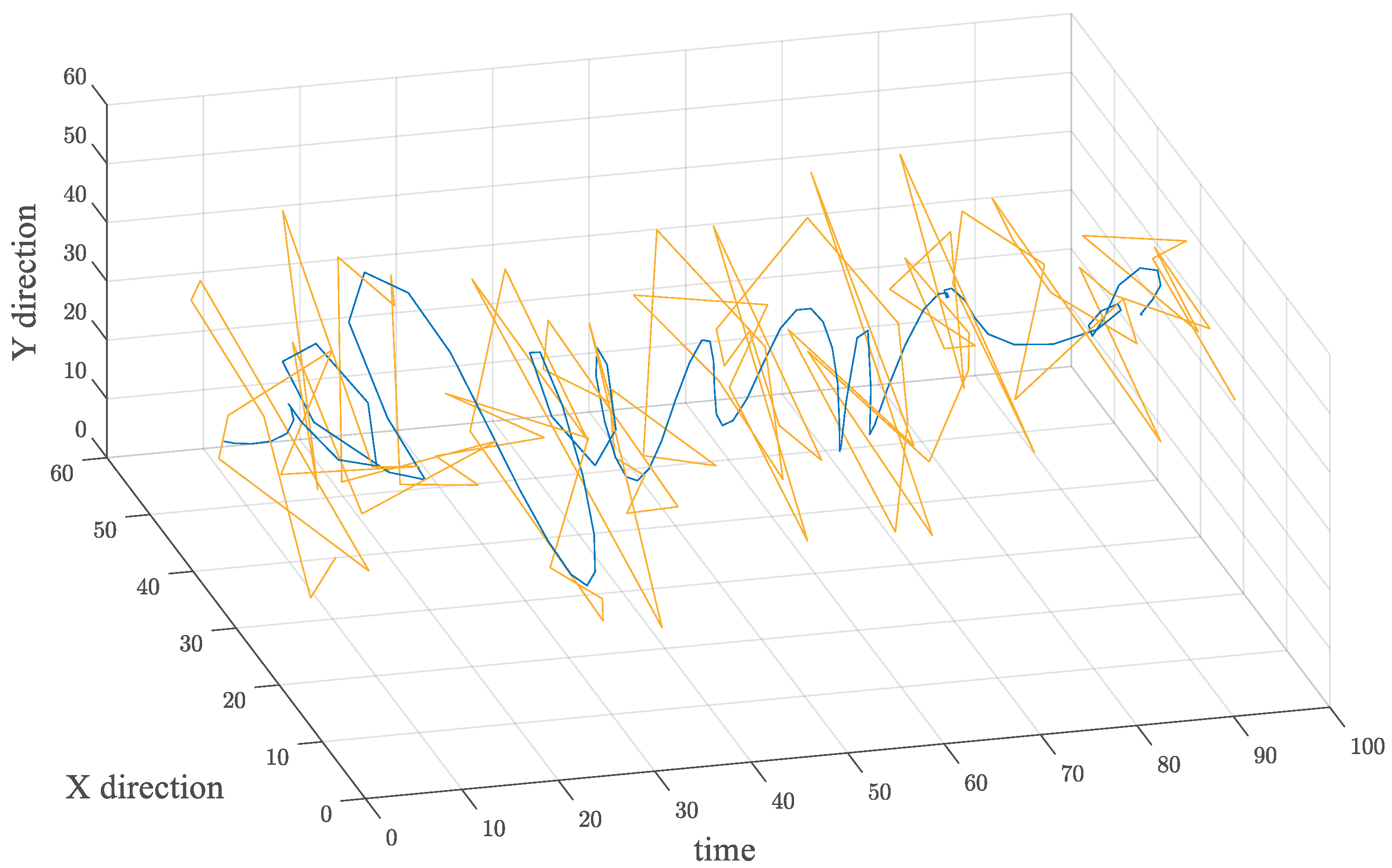
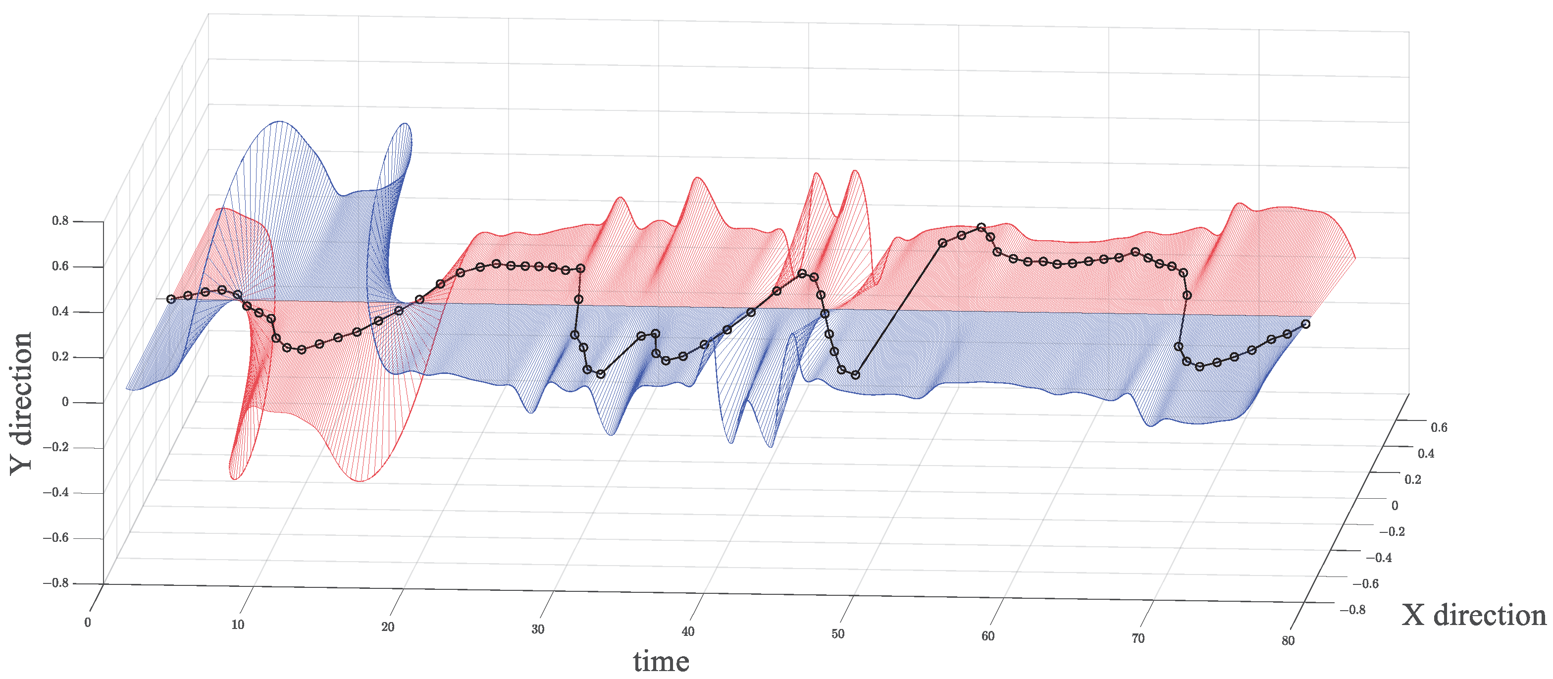
Figure 1 shows an example of two-dimensional series. Figure 2 illustrates the curve surface made of base angle series and the red part is the positive direction while the blue part is the negative direction. In fact, only those base angle series corresponding to the points on the black line were meaningful. For a better display, the angle series between the real base angle series was obtained via spline interpolation. 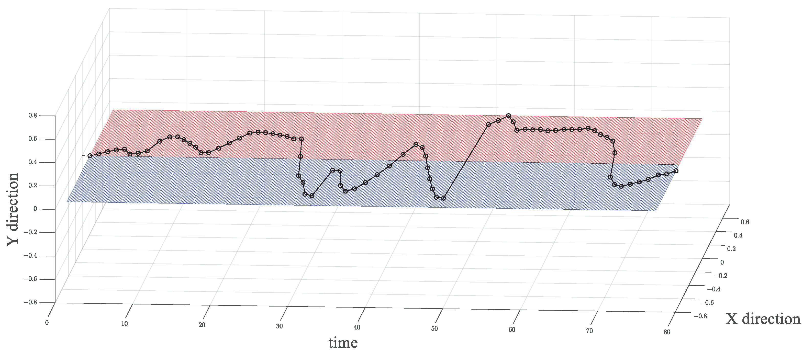Figure 3 illustrates the “flattened” surface and the signal. At time period of 7 to 15 s (the time difference for each point on the black line is one second), although the “trend” of the curve was “downward” according to Figure 1, the change rate of phase of those points was not steep so that those points remained in positive direction in Figure 3.

3.3. Complex Envelope-like Series and Sifting Process

Given the definition of extremum-like points of complex series, the upper and lower envelope-like series of signals could be computed. Specifically, link the series composed of a real part of the maximum-like series and the series composed of an imaginary part separately via cubic spline line (blue line in Figure 4), then combine the two series as the upper envelope-like series, and the same for the lower envelope-like series (red line in Figure 4). The pseudocode for computing complex envelope-like series is shown in Algorithm 1.

Algorithm 1: Complex envelope-like series.

Input: Complex Series Z

Output: Upper and lower envelope-like series U, D

$r\leftarrow abs\left(Z\right)$;

$\theta \leftarrow ang\left(Z\right)$;

$B\left(0\right)\leftarrow \theta \left(0\right)$;

$U_{re}\leftarrow spline\left(Re\left(MA\right),length\left(Z\right)\right)$;

$U_{im}\leftarrow spline\left(Im\left(MA\right),length\left(Z\right)\right)$;

$D_{re}\leftarrow spline\left(Re\left(MI\right),length\left(Z\right)\right)$;

$D_{im}\leftarrow spline\left(Im\left(MI\right),length\left(Z\right)\right)$;

$U\leftarrow complex\left(U_{re},U_{im}\right)$;

$D\leftarrow complex\left(D_{re},D_{im}\right)$;

As for the first sifting process, let $m_n^1$ be the mean series of upper and lower envelope-like series (blue line in Figure 5) and the minus between the signal series $z_n$ and $m_n^1$ is the first component series $h_n^1$. The same process was repeated on $h_n^1$ to obtain $h_n^2$. For the $k^{\mathrm{th}}$ sifting process, the mean value series of envelope-like series was $m_n^k$, the component series was $h_n^k$. Let SD be the standard deviation as

$$SD=\sum _n\frac{{\left|h_n^k-h_n^{k-1}\right|}^2}{{\left|h_n^{k-1}\right|}^2}$$

(7)

when $SD<\sigma$, $\sigma$ was a predetermined value, the component series $h_n^k$ was the first IMF $c_n^1$. The same as the original EMD, $c_n^k,k=1,2,3,\dots$ and $r_n$ was calculated. The signal series was composed of those IMFs and the residual was

$$z_n=\sum _k{c}_n^k+r_n$$

(8)

4. Trajectory Data Mode Decomposition

In order to test the proposed decomposition method, two sets of trajectory series were collected. One was collected indoors, which included frequent direction changes, while the other set was collected outdoors and consisted of several different motion modes.

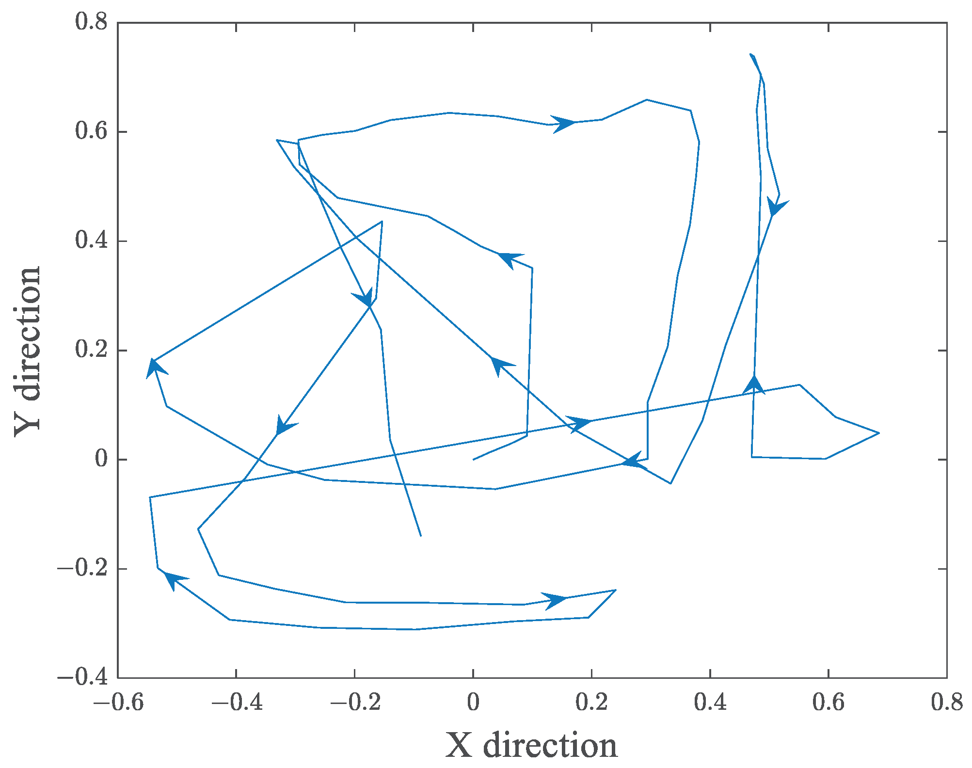
4.1. Indoor Trajectory Decomposition Experiment

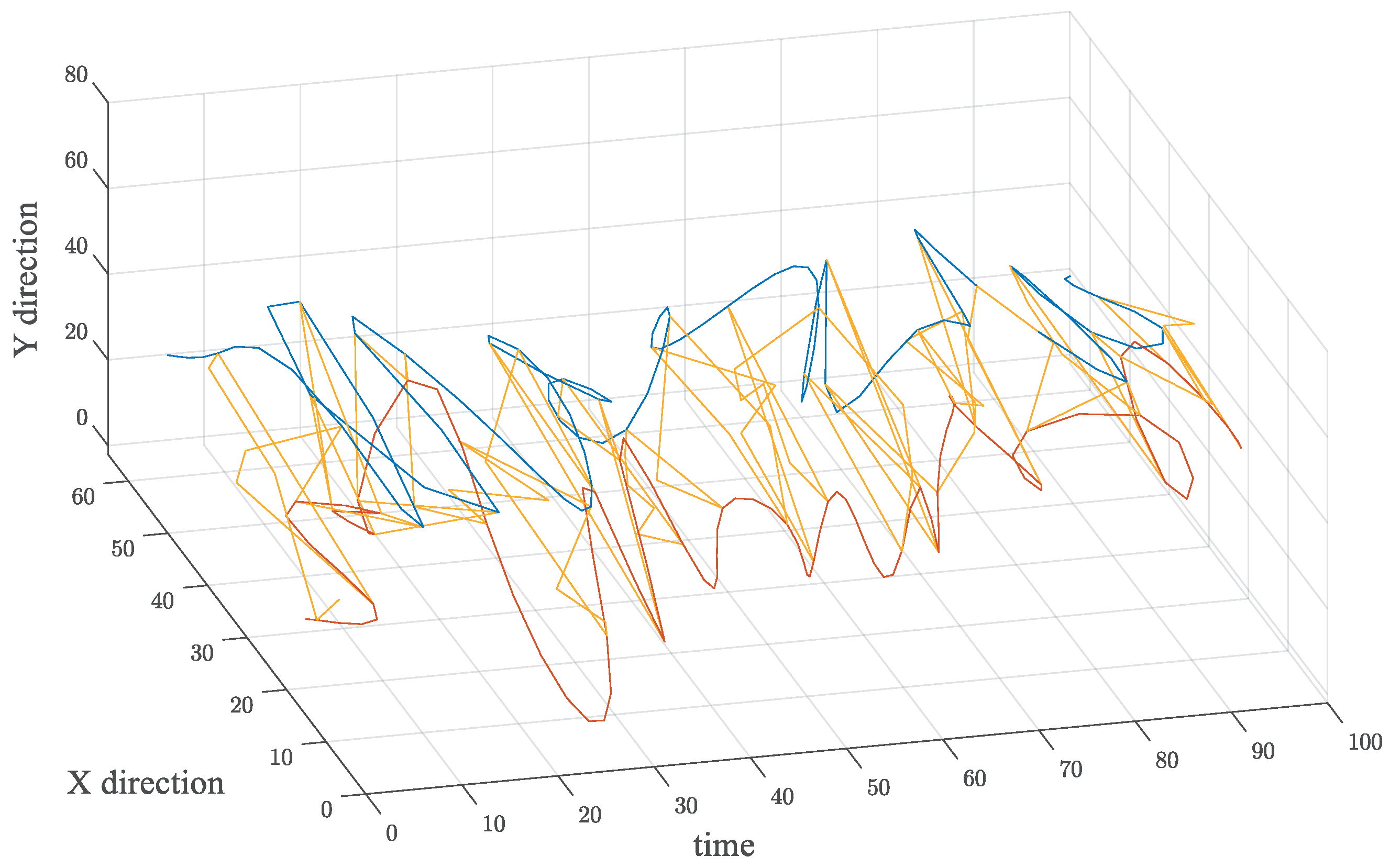
A walking trajectory was used to test the complex empirical mode decomposition. The data were collected in an about 25 m² room and the direction of the trajectory changed frequently. In the experiment, the tester held a device combination with mounted camera and single board computer and walked freely in the room. In the meantime, the trajectory of the tester was computed via ORB-SLAM. Each point of the trajectory includes the timestamps, x coordinate and y coordinate. The original signal was formed by linking the points of the trajectory in time order and was shown in Figure 6.

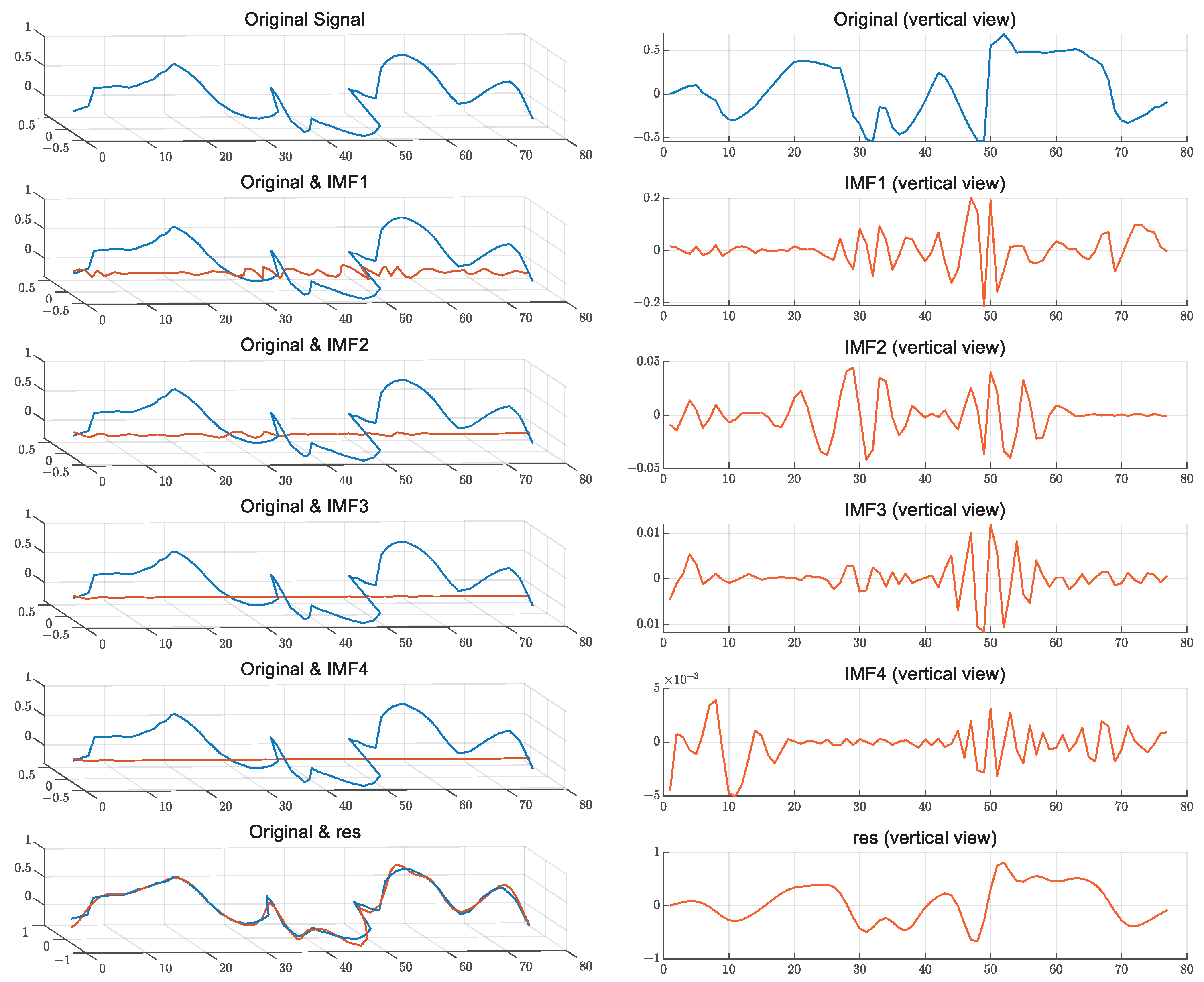
Figure 7 demonstrates the decomposition results of the indoor trajectory. Blue lines illustrate the original series in time-x-y coordinates, orange lines illustrate the IMFs and residual. The left column is the axonometric projection graph of the original series, the IMF series and the residual series. Each sub-figure in the right column is the vertical view of the original series, the IMF series or the residual series.

The residual series is close to the original series while IMFs extract the oscillation modes of the original series which indicate the characters of the trajectory. The oscillation amplitude of IMF1 and IMF2 were relatively significant. In IMF1, the oscillations mainly occurred when the trajectory’s direction changed rapidly. In IMF2, the oscillations appeared at the edge of significant changes in the trajectory direction and at the beginning of trajectories with mild direction changes. The oscillations of IMF3 indicate that the right edge of the trajectory segment with rapid direction change has a different intrinsic mode compared to the left edge. The oscillations of IMF4 mainly appeared at the beginning and ending segments of the trajectory.

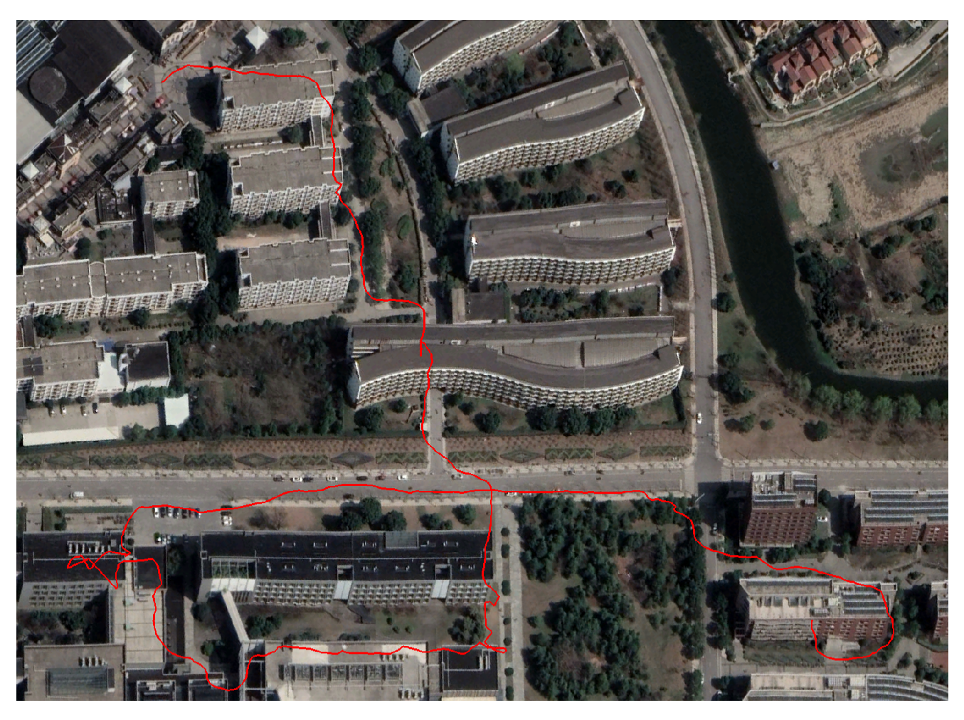
4.2. Outdoor Trajectory Decomposition Experiment

Another walking trajectory of a participant was used to test the performance of the CEMD. In the experiment, the tester walked in the campus of Tongji University and held a mobile GPS receive device to collect the GPS log data. The latitude, the longitude and the timestamps of the GPS logs were used and linked in time order to form the original signal. The GPS devices recorded 827 points in 15 min and 36 s and the trajectory is 1.3 km long. In the recorded trajectory (Figure 8), there were longer straight sections, some turns and occasional back-and-forth movements at certain locations.

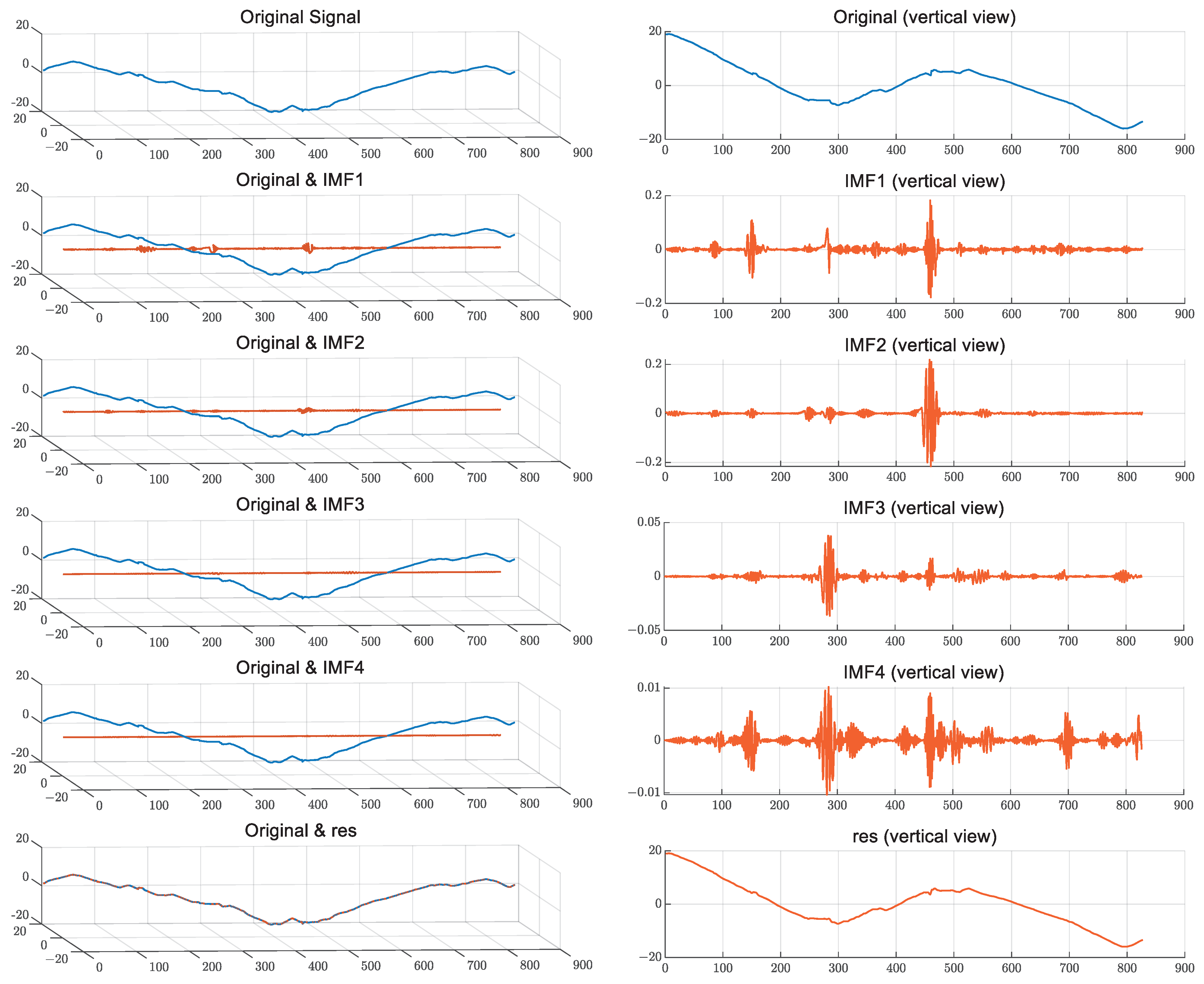
Figure 9 demonstrates the decomposition results of the outdoor trajectory. The blue lines illustrate the original series and the orange lines illustrate the IMFs and the residual. The left column is the axonometric projection graph and the right column is the vertical view. In the left column, the amplitudes of the IMFs in the left column of the figure were 15 times larger than the actual values because the actual amplitudes were too small compared to the original series and the residual, making them not clearly visible in the figure.

The IMFs in Figure 9 show that the oscillation modes occurred in some particular time period and the oscillations were very distinct. The oscillations (especially in IMF1) related to the moments when the tester was lingering in a certain spot while the smoother parts of the IMF1 correspond to the times when the tester was walking at a steady pace. The oscillations of IMF2 were also related to the most significant direction changes in the trajectory. The oscillations of IMF3 were related to the first right-angle turn of the original trajectory. The oscillations of IMF4 were related to almost every significant turn of the original trajectory. That may indicate that all of them have similar intrinsic mode components.

The decomposition results of the outdoor trajectory contain two major problems. First, the effects of small-scale directional oscillations of the trajectory were ignored by the decomposition algorithm due to the spatial scale discrepancy with the trajectory. Even though the IMFs in the left column of Figure 9 were 15 times larger than the actual values, the oscillations were still not apparent. Second, it can be found that several distinct intrinsic modes appeared in the same IMF and that was not just a typical modal mixing phenomenon. To analyze it theoretically, the mean series obtained from the envelope series does not always have the same phase angle as the series being decomposed at each moment. Therefore, subtracting the mean series from the series may introduce new oscillations.

One possible solution to the first problem is to have the original data be differentiated before decomposition, inspired by a similar operation used in the classical Empirical Mode Decomposition algorithm when dealing with the problem of insufficient extrema points in the original signals. Regarding the second issue, an informal solution was proposed.

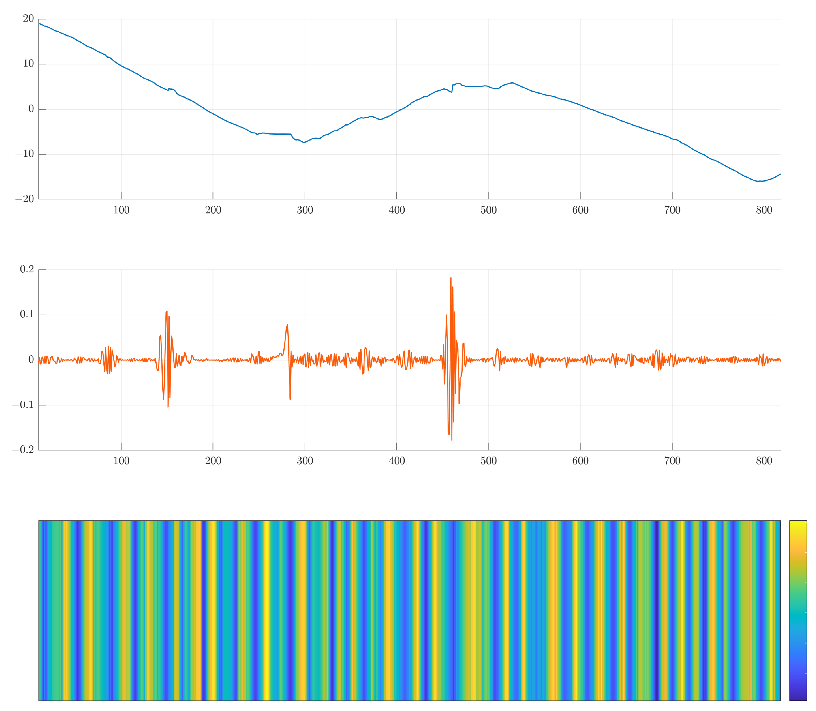
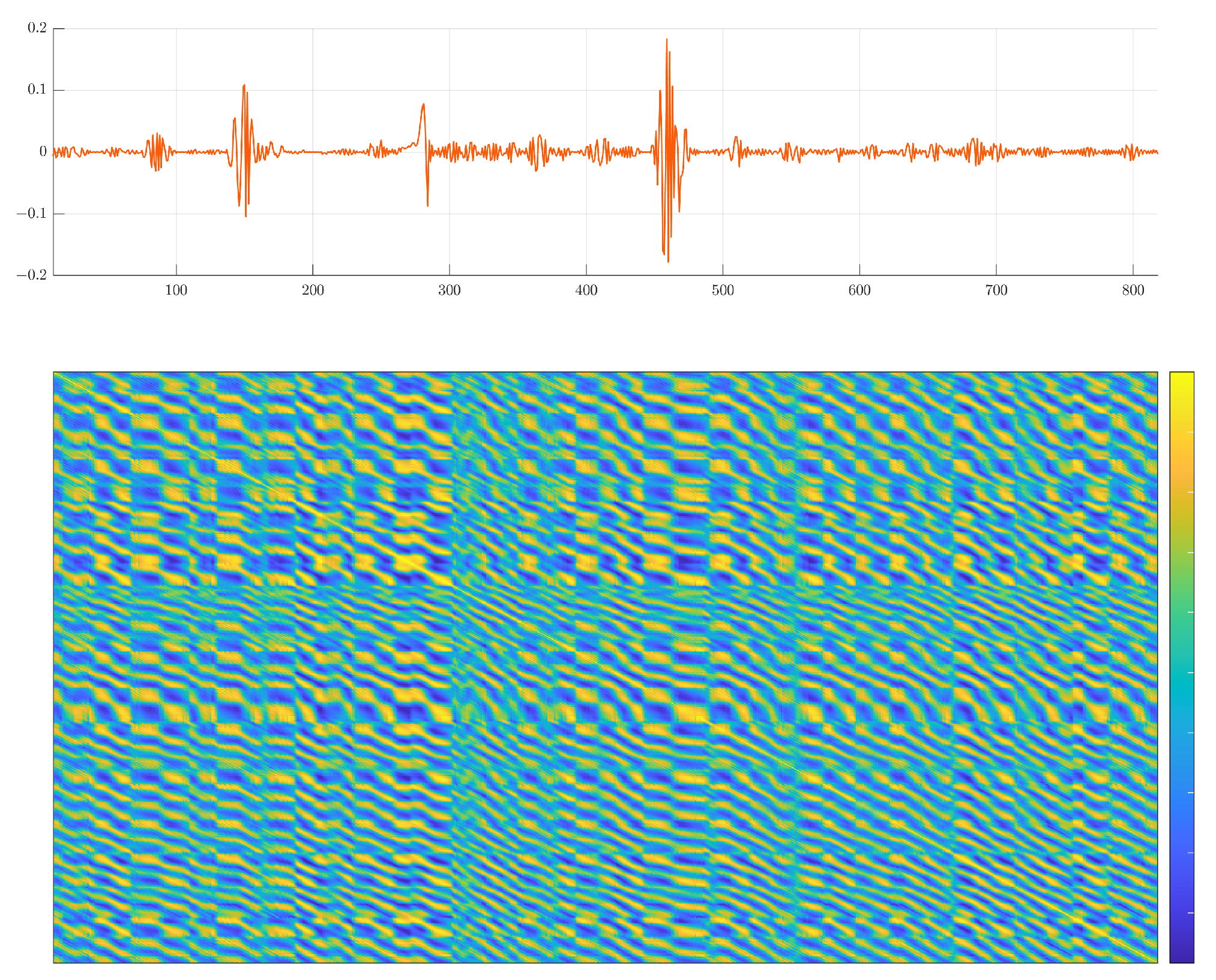
Figure 10 demonstrates the shifting self-correlation analysis of IMF1 of the outdoor trajectory. A sliding window with a fixed width is used to move forward with a step size of 1 on the IMF1 series so that several subunits were obtained. The matrix was formed by calculating the cross-correlation coefficients between those subunits. There are several vertical (or horizontal) boundary lines present on the heatmap of the matrix. By examining the correlation coefficients near the diagonal of the heatmap, it can be observed that there is a high level of correlation within the IMF segment between each boundary line. By summing up all the elements in each column of the matrix, a comprehensive correlation index vector can be obtained. As shown in Figure 11, it can be used to measure the uniqueness of each segment compared to the rest of the series. Those “unique segments” can be selected as an intrinsic mode of the original series. In Figure 11, the segment where the most significant oscillations occurs could be considered as such an intrinsic mode. In fact, this segment also corresponded to the most significant directional changes in the trajectory.

5. Discussion and Conclusions

To achieve the empirical mode decomposition of multivariate data, a complex EMD method was proposed in which an intermediate variable and a base angle were introduced. Then the multivariatetemporal series, represented as a complex number, could be mapped onto a curved surface generated by the base angle series. The envelope-like function of the complex series is obtained by determining the extremum-like point of the series on the surface. Then, following the sifting step of the classic empirical mode decomposition method, the intrinsic mode functions of the complex series are obtained. Compared to the existing multivariate EMD method that requires generating too many projection directions, the proposed method avoided significant computational burden and appeared to be more flexible and adaptive.

However, the experiment showed that the method does not effectively extract a small spatial-scale oscillation mode from large spatial-scale data such as traffic trajectory and the algorithm itself might cause additional oscillations that are difficult to eliminate completely. Regarding the first problem, the differencing operation could be applied to the raw data as preprocessing. An informal solution to the second problem was introduced in Section 4.2.

The application of the complex EMD on trajectory data indicates that the extracted IMFs can help to distinguish time series segments with different motion characteristics. In addition, the proposed method has potential with respect to decomposition of multivariate traffic and transportation data for the application such as traffic data denoising, pattern recognition, traffic flow dynamics evaluation, traffic prediction, etc.