
Gearbox Fault Diagnosis Based on Gramian Angular Field and CSKD-ResNeXt
Abstract
:1. Introduction
1.1. Motivation
1.2. Analysis of Related Works
1.3. Contributions
- i.
- In this paper, a Gramian image is used as the sample diagram of model input. After comparing the performance of GADF (Gramian angular difference field) and GASF (Gramian angular summation field), one with good effect is selected to process one-dimensional vibration signals, and the output two-dimensional sample image is used to express time-dependent signal characteristics.
- ii.
- The 7 × 7 convolutional kernel in the backbone of the ResNeXt model was decomposed into three 3 × 3 convolutional kernels, which reduced the feature extraction ambiguity caused by a large convolutional kernel and improved model semantic capability. After receiving vibration signals, the convolution kernel can extract more accurate and detailed feature information and improve the diagnostic accuracy.
- iii.
- For the purpose of feature communication, channel shuffle is added to the group convolution part to break the isolation between channels and exchange data. The data flow in the model is enriched to obtain a more competitive feature-mining capability. In addition, the process of fault identification and classification is demonstrated by using t-SNE visual dimension reduction.
2. Methods
2.1. The GAF
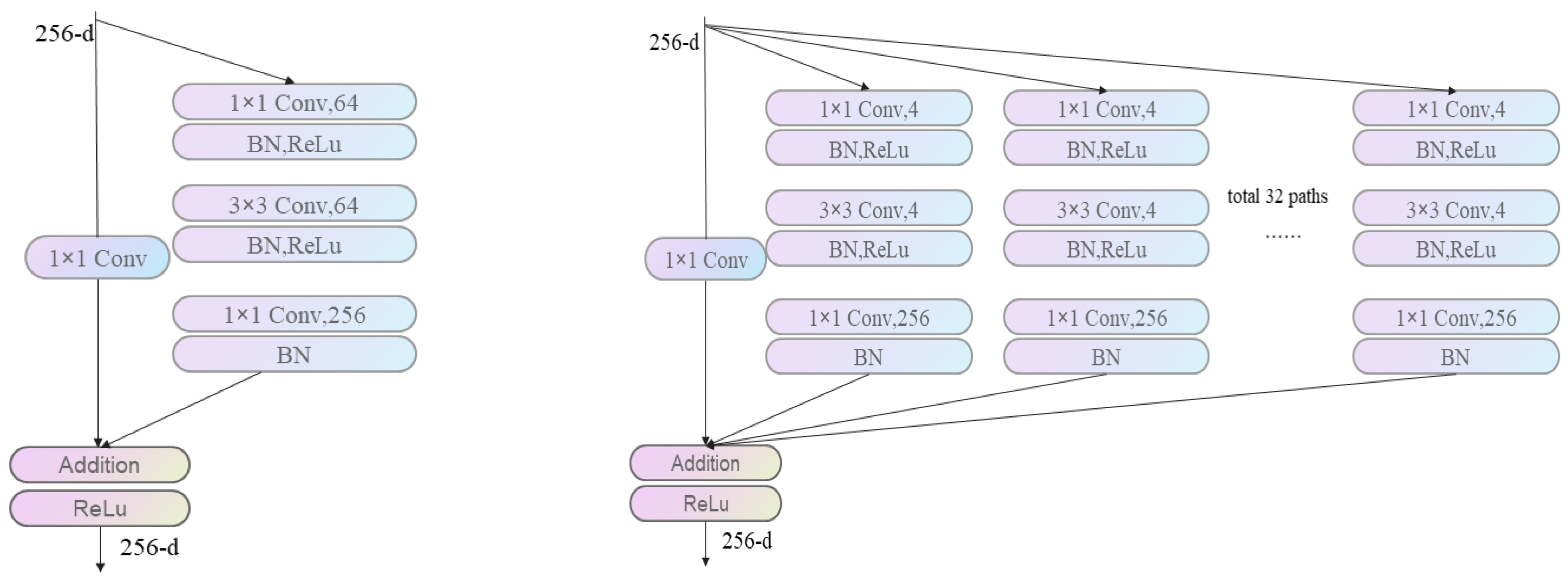
2.2. ResNeXt
- (1)
- Channel Shuffle
- i.
- Reshape: the input layer is assumed to be divided into g groups, and the total number of channels is g × n. The input channel dimension is reshaped into two dimensions (g,n), which represent the number of convolution groups and the number of channels contained in each convolution group.
- ii.
- Transpose: transpose two extended dimensions into (n,g).
- iii.
- Flatten: the transposed channel flatten is reshaped into dimension g × n, and channel shuffle can be finished.
- (2)
- Kernel Decomposed
2.3. Establishing the CSKD-ResNext Network
3. Data Description
3.1. Datasets
3.2. Experimental Platform Setting
4. Analysis of Model Results
4.1. Model Verification
4.2. t-SNE Visualization
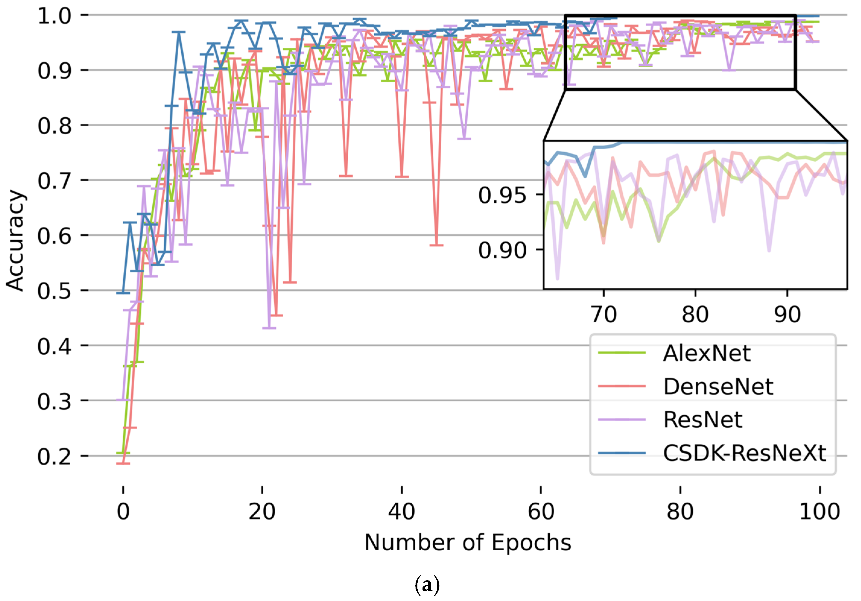
4.3. Contrast of Classical Model
5. Conclusions
Author Contributions
Funding
Data Availability Statement
Conflicts of Interest
References
- Wang, R.; Zhan, X.; Bai, H.; Dong, E.; Cheng, Z.; Jia, X. A Review of Fault Diagnosis Methods for Rotating Machinery Using Infrared Thermography. Micromachines 2022, 13, 1644. [Google Scholar] [CrossRef] [PubMed]
- Lu, L.; He, Y.; Ruan, Y.; Yuan, W. An optimized stacked diagnosis structure for fault diagnosis of wind turbine planetary gearbox. Meas. Sci. Technol. 2021, 32, 75102. [Google Scholar] [CrossRef]
- Guo, Y.J.; Jiang, S.F.; Yang, Y.D.; Jin, X.H.; Wei, Y.D. Gearbox Fault Diagnosis Based on Improved Variational Mode Extraction. Sensors 2022, 22, 1779. [Google Scholar] [CrossRef] [PubMed]
- Sohaib, M.; Munir, S.; Islam MM, M.; Shin, J.; Tariq, F.; Rashid SM, M.; Kim, J. Gearbox fault diagnosis using improved feature representation and multitask learning. Front. Energy Res. 2022, 10, 998760. [Google Scholar] [CrossRef]
- Schoen, R.R.; Habetler, T.G.; Kamran, F.; Bartfield, R.G. Motor bearing damage detection using stator current monitoring. IEEE Trans. Ind. Appl. 1995, 31, 1274–1279. [Google Scholar] [CrossRef]
- Zhong, R.Y.; Xu, X.; Klotz, E.; Newman, S.T. Intelligent Manufacturing in the Context of Industry 4.0: A Review. Engineering 2017, 3, 616–630. [Google Scholar] [CrossRef]
- Lee, J.; Wu, F.; Zhao, W.; Ghaffari, M.; Liao, L.; Siegel, D. Prognostics and health management design for rotary machinery systems—Reviews, methodology and applications. Mech. Syst. Signal Process. 2014, 42, 314–334. [Google Scholar] [CrossRef]
- Alvarez, E.J.; Ribaric, A.P. An improved-accuracy method for fatigue load analysis of wind turbine gearbox based on SCADA. Renew. Energy 2018, 115, 391–399. [Google Scholar] [CrossRef]
- Li, H.; Feng, G.; Zhen, D.; Gu, F.; Ball, A.D. A normalized frequency-domain energy operator for broken rotor bar fault diagnosis. IEEE Trans. Instrum. Meas. 2021, 70, 3500110. [Google Scholar] [CrossRef]
- Li, C.; Zhang, S.; Qin, Y.; Estupinan, E. A systematic review of deep transfer learning for machinery fault diagnosis. Neurocomputing 2020, 407, 121–135. [Google Scholar] [CrossRef]
- Contin, A.; D’Orlando, S.; Fenu, G.; Menis, R.; Milo, S.; Parisini, T. Experiments on actuator fault diagnosis: The case of a nonlinearly controlled AC motor. In Proceedings of the European Control Conference (ECC), Porto, Portugal, 4–7 September 2001; pp. 2747–2752. [Google Scholar] [CrossRef]
- Lecun, Y.; Bengio, Y.; Hinton, G. Deep learning. Nature 2015, 521, 436–444. [Google Scholar] [CrossRef] [PubMed]
- You, D.; Gao, X.; Katayama, S. Multisensor Fusion System for Monitoring High-Power Disk Laser Welding Using Support Vector Machine. IEEE Trans. Ind. Inform. 2014, 10, 1285–1295. [Google Scholar] [CrossRef]
- Tian, J.; Morillo, C.; Azarian, M.H.; Pecht, M. Motor Bearing Fault Detection Using Spectral Kurtosis-Based Feature Extraction Coupled With K-Nearest Neighbor Distance Analysis. IEEE Trans. Ind. Electron. 2016, 63, 1793–1803. [Google Scholar] [CrossRef]
- Shevchik, S.A.; Saeidi, F.; Meylan, B.; Wasmer, K. Prediction of Failure in Lubricated Surfaces Using Acoustic Time–Frequency Features and Random Forest Algorithm. IEEE Trans. Ind. Inform. 2017, 13, 1541–1553. [Google Scholar] [CrossRef]
- Lei, Y.; Karimi, H.R.; Chen, X. A novel self-supervised deep LSTM network for industrial temperature prediction in aluminum processes application. Neurocomputing 2022, 502, 177–185. [Google Scholar] [CrossRef]
- Arel, I.; Rose, D.C.; Karnowski, T.P. Deep Machine Learning—A New Frontier in Artificial Intelligence Research [Research Frontier]. IEEE Comput. Intell. Mag. 2010, 5, 13–18. [Google Scholar] [CrossRef]
- Saxena, A.; Parey, A.; Chouksey, M. Time varying mesh stiffness calculation of spur gear pair considering sliding friction and spalling defects. Eng. Fail. Anal. 2016, 70, 200–211. [Google Scholar] [CrossRef]
- Sanchez, H.; Escobet, T.; Puig, V.; Odgaard, P.F. Fault Diagnosis of an Advanced Wind Turbine Benchmark Using Interval-Based ARRs and Observers. IEEE Trans. Ind. Electron. 2015, 62, 3783–3793. [Google Scholar] [CrossRef]
- Sun, R.; Yang, Z.; Yang, L.; Qiao, B.; Chen, X.; Gryllias, K. Planetary gearbox spectral modeling based on the hybrid method of dynamics and LSTM. Mech. Syst. Signal Process. 2020, 138, 106611. [Google Scholar] [CrossRef]
- Shanbr, S.; Elasha, F.; Elforjani, M.; Teixeira, J. Detection of natural crack in wind turbine gearbox. Renew. Energy 2018, 118, 172–179. [Google Scholar] [CrossRef]
- Wang, J.; Peng, Y.; Qiao, W.; Hudgins, J.L. Bearing Fault Diagnosis of Direct-Drive Wind Turbines Using Multiscale Filtering Spectrum. IEEE Trans. Ind. Appl. 2017, 53, 3029–3038. [Google Scholar] [CrossRef]
- Lv, Y.; Guan, N.; Liu, J.; Cai, T. The fault diagnosis of rolling bearing in gearbox of wind turbines based on second generation wavelet. In Proceedings of the International Conference on Wavelet Analysis and Pattern Recognition, Lanzhou, China, 13–16 July 2014; pp. 43–49. [Google Scholar] [CrossRef]
- Lopez-Ramirez, M.; Romero-Troncoso, R.J.; Morinigo-Sotelo, D.; Duque-Perez, O.; Ledesma-Carrillo, L.M.; Camarena-Martinez, D.; Garcia-Perez, A. Detection and diagnosis of lubrication and faults in bearing on induction motors through STFT. In Proceedings of the International Conference on Electronics, Communications and Computers (CONIELECOMP), Cholula, Mexico, 24–26 February 2016; pp. 13–18. [Google Scholar] [CrossRef]
- Tang, G.; Wang, Y.; Huang, Y.; Wang, H. Multiple time-frequency curve classification for tacho-less and resampling-less compound bearing fault detection under time-varying speed conditions. IEEE Sens. J. 2021, 21, 5091–5101. [Google Scholar] [CrossRef]
- Zeng XJ Yang, M.; Bo, Y.F. Gearbox oil temperature anomaly detection for wind turbine based on sparse Bayesian probability estimation. Int. J. Electr. Power Energy Syst. 2020, 123, 106233. [Google Scholar] [CrossRef]
- Wang, Z.Y.; Li, G.S.; Yao, L.G.; Qi, X.L.; Zhang, J. Data-driven fault diagnosis for wind turbines usingmodified multiscale fluctuation dispersion entropy and cosine pairwise-constrainedsupervised manifold mapping. Knowl.-Based Syst. 2021, 228, 107276. [Google Scholar] [CrossRef]
- Toma, R.N.; Kim, J.M. Bearing Fault Classification of Induction Motors Using Discrete Wavelet Transform and Ensemble Machine Learning Algorithms. Appl. Sci. 2020, 10, 5251. [Google Scholar] [CrossRef]
- Pang, J.S.; Chen, Y.M.; He, S.Z.; Qiu, H.H.; Wu, C.L.; Mao, L.B. Classification of Friction and Wear State of Wind Turbine Gearboxes Using Decision Tree and Random Forest Algorithms. J. Tribol. -Trans. ASME 2021, 143, 91702. [Google Scholar] [CrossRef]
- Wang, H.; Liu, Z.; Peng, D.; Qin, Y. Understanding and Learning Discriminant Features based on Multiattention 1DCNN for Wheelset Bearing Fault Diagnosis. IEEE Trans. Ind. Inform. 2020, 16, 5735–5745. [Google Scholar] [CrossRef]
- Yu, J.; Zhou, X. One-Dimensional Residual Convolutional Autoencoder Based Feature Learning for Gearbox Fault Diagnosis. IEEE Trans. Ind. Inform. 2020, 16, 6347–6358. [Google Scholar] [CrossRef]
- Xingkang, Z.; Jianbo, Y. Gearbox Fault Diagnosis Based on One-dimension Residual Convolutional Auto-encoder. J. Mech. Eng. 2020, 56, 96–108. [Google Scholar] [CrossRef]
- Yang, S.; Liu, L.; Zhou, J.; Zhao, Y.; Hua, G.; Sun, H.; Zheng, N. Robust and Efficient Star Identification Algorithm based on 1-D Convolutional Neural Network. IEEE Trans. Aerosp. Electron. Syst. 2022, 58, 4156–4167. [Google Scholar] [CrossRef]
- Xu, H.; Cai, C.Z.; Chi, Y.L.; Zhang, N. Fault diagnosis of gearbox based on adaptive wavelet de-noising and convolution neural network. Adv. Mech. Eng. 2023, 15, 16878132231157186. [Google Scholar] [CrossRef]
- Wang, L.-H.; Zhao, X.-P.; Wu, J.-X.; Xie, Y.-Y.; Zhang, Y.-H. Motor Fault Diagnosis Based on Short-time Fourier Transform and Convolutional Neural Network. Chin. J. Mech. Eng. 2017, 30, 1357–1368. [Google Scholar] [CrossRef]
- Zhang, Y.; Xing, K.; Bai, R.; Sun, D.; Meng, Z. An enhanced convolutional neural network for bearing fault diagnosis based on time–frequency image. Measurement 2020, 157, 107667. [Google Scholar] [CrossRef]
- Huang, D.; Zhang, W.A.; Guo, F.; Liu, W.; Shi, X. Wavelet Packet Decomposition-Based Multiscale CNN for Fault Diagnosis of Wind Turbine Gearbox. IEEE Trans. Cybern. 2023, 53, 443–453. [Google Scholar] [CrossRef] [PubMed]
- Liu, H.; Mi, X.; Li, Y. Smart multi-step deep learning model for wind speed forecasting based on variational mode decomposition, singular spectrum analysis, LSTM network and ELM. Energy Convers. Manag. 2018, 159, 54–64. [Google Scholar] [CrossRef]
- Gu, J.; Wang, Z.; Kuen, J.; Ma, L.; Shahroudy, A.; Shuai, B.; Liu, T.; Wang, X.; Wang, G.; Cai, J.; et al. Recent advances in convolutional neural networks. Pattern Recognit. 2018, 77, 354–377. [Google Scholar] [CrossRef]
- Shin, H.C.; Roth, H.R.; Gao, M.; Lu, L.; Xu, Z.; Nogues, I.; Yao, J.; Mollura, D.; Summers, R.M. Deep Convolutional Neural Networks for Computer-Aided Detection: CNN Architectures, Dataset Characteristics and Transfer Learning. IEEE Trans. Med. Imaging 2016, 35, 1285–1298. [Google Scholar] [CrossRef]
- Babu, T.N.; Ali PS, N.; Prabha, D.R.; Mohammed, V.N.; Wahab, R.S.; Vijayalakshmi, S. Fault Diagnosis in Bevel Gearbox Using Coiflet Wavelet and Fault Classification Based on ANN Including DNN. Arab. J. Sci. Eng. 2022, 47, 15823–15849. [Google Scholar] [CrossRef]
- Zhang, K.; Chen, J.; Zhang, T.; Zhou, Z. A Compact Convolutional Neural Network Augmented with Multiscale Feature Extraction of Acquired Monitoring Data for Mechanical Intelligent Fault Diagnosis. J. Manuf. Syst. 2020, 55, 273–284. [Google Scholar] [CrossRef]
- Krizhevsky, A.; Sutskever, I.; Hinton, G.E. ImageNet classification with deep convolutional neural networks. Commun. ACM 2017, 60, 84–90. [Google Scholar] [CrossRef]
- Gu, F.C. Application of the convolutional neural network in partial discharge spectrum recognition of power apparatus. IET Sci. Meas. Technol. 2023, 1–10. [Google Scholar] [CrossRef]
- O’Shea, T.J.; Roy, T.; Clancy, T.C. Over-the-Air Deep Learning Based Radio Signal Classification. IEEE J. Sel. Top. Signal Process. 2018, 12, 168–179. [Google Scholar] [CrossRef]
- Liu, J.; Wang, Y.C.; Siong, T.C.; Li, X.J.; Zhao, L.P.; Wei, F.R. On the combination of adaptive neuro-fuzzy inference system and deep residual network for improving detection rates on intrusion detection. PLoS ONE 2022, 17, e0278819. [Google Scholar] [CrossRef]
- Xie, S.N.; Girshick, R.; Dollar, P.; Tu, Z.W.; He, K.M. Aggregated residual transformations for deep neural networks. In Proceedings of the 30th IEEE/CVF Conference on Computer Vision and Pattern Recognition (CVPR), Honolulu, HI, USA, 21–26 July 2017. [Google Scholar] [CrossRef]
- Gao, C.; Wu, J.; Yu, H.; Yin, J.; Guo, S. FIRN: A Novel Fish Individual Recognition Method with Accurate Detection and Attention Mechanism. Electronics 2022, 11, 3459. [Google Scholar] [CrossRef]
- Zhang, Y.T.; Zhuo, L.; Ma, C.J.; Zhang, Y. Abnormal Object Detection in X-ray Images with Self-normalizing Channel Attention and Efficient Data Augmentation; In Proceedings of the International Workshop on Advanced Imaging Technology (IWAIT), Hong Kong, China, 4–6 January 2022. [CrossRef]
- Wang, G.W.; Wang, J.X.; Yu, H.Y.; Sui, Y.Y. Research on Identification of Corn Disease Occurrence Degree Based on Improved ResNeXt Network. Int. J. Pattern Recognit. Artif. Intell. 2022, 36, 2250005. [Google Scholar] [CrossRef]
- Fang, J.; Xu, C.; Wang, C.; Li, H. Dynamic Gesture Recognition Based On Multimodal Fusion Model. In Proceedings of the 2021 20th International Conference on Ubiquitous Computing and Communications (IUCC/CIT/DSCI/SmartCNS), London, UK, 20–22 December 2021; pp. 172–177. [Google Scholar] [CrossRef]
- Zhou, Y.J.; Long, X.Y.; Sun, M.W.; Chen, Z.Q. Bearing fault diagnosis based on Gramian angular field and DenseNet. Math. Biosci. Eng. 2022, 19, 14086–14101. [Google Scholar] [CrossRef]
- Xi, C.P.; Liu, R.Q. Detection of Small Floating Target on Sea Surface Based on Gramian Angular Field and Improved EfficientNet. Remote Sens. 2022, 14, 4364. [Google Scholar] [CrossRef]
- Xue, Y.M.; Huang, W.M.; Yang, C. Hyperspectral image classification based on gramian angular fields encoding. In Proceedings of the Canadian Conference on Electrical and Computer Engineering (CCECE), Halifax, NS, Canada, 18–20 September 2022. [Google Scholar] [CrossRef]
- Dong, S.J.; Li, Y.; Zhu, P.; Pei, X.W.; Pan, X.J.; Xu, X.Y.; Liu, L.H.; Xing, B.; Hu, X.L. Rolling bearing performance degradation assessment based on singular value decomposition-sliding window linear regression and improved deep learning network in noisy environment. Meas. Sci. Technol. 2022, 33, 045015. [Google Scholar] [CrossRef]
- Zhang, X.; Zhou, X.Y.; Lin, M.X.; Sun, J. ShuffleNet: An Extremely Efficient Convolutional Neural Network for Mobile Devices; In Proceedings of the 31st IEEE/CVF Conference on Computer Vision and Pattern Recognition (CVPR), Salt Lake City, UT, USA, 18–23 June 2018. [CrossRef]
- Shao, S.; Mcaleer, S.; Yan, R.; Baldi, P. Highly Accurate Machine Fault Diagnosis Using Deep Transfer Learning. IEEE Trans. Ind. Inform. 2019, 15, 2446–2455. [Google Scholar] [CrossRef]
- Diederik, K.; Ba, J.L. ADAM: A method for stochastic optimization. AIP Conf. Proc. 2014, 1631, 58–62. [Google Scholar] [CrossRef]
- Lu, W.P.; Yan, X.F. Variable-weighted FDA combined with t-SNE and multiple extreme learning machines for visual industrial process monitoring. ISA Trans. 2022, 122, 163–171. [Google Scholar] [CrossRef] [PubMed]


| Fault Diagnosis Methods | Diagnostic Limitations | Related Researches | |
|---|---|---|---|
| Model-based fault diagnosis method | Fault mechanism and physical models are combined to analyze the nature of the fault but are more applicable to systems that can be modeled accurately. | Saxena A et al., (2016) [18] Sanchez H et al., (2015) [19] Sun et al., (2020) [20] | |
| Signal processing-based fault diagnosis method | It does not need to rely on a large amount of data and also has better performance for signals with low SNR. However, the signal processing method is localized, and different research objects usually correspond to different fault diagnosis indexes. | Shanbr S et al., (2018) [21] Wang et al., (2017) [22] Lv et al., (2014) [23] Misael Lopez-Ramirez et al., (2016) [24] Tang et al., (2021) [25] | |
| Traditional machine learning-based fault diagnosis method | Machine learning algorithms inject intelligence into the field of fault diagnosis, but the feature extraction process and classification task are two independent subjects. How to extract the optimal features is still a problem that many researchers are paying attention to. | Zeng et al., (2020) [26] Wang et al., (2021) [27] Toma R N et al., (2021) [28] Pang et al., (2021) [29] | |
| Deep-learning-based fault diagnosis method | One-dimensional signal as input | It has low computational complexity and is suitable for real-time and low-cost applications, but the applicability of one-dimensional signals and most network structures is poor. The internal setup of the model is the problem facing to improve the applicability of one-dimensional diagnostic model. | Wang et al., (2019) [30] Yu et al., (2020) [31] Zhou et al., (2020) [32] Yang et al., (2022) [33] |
| The signal is converted into a two-dimensional image as input | The model can learn the most representative fault features by combining the signal preprocessing technology with the algorithm with excellent performance in the field of image recognition, but this method is restricted by the amount of data and training cost. | Xu et al., (2023) [34] Wang et al., (2017) [35] Zhang et al., (2020) [36] Huang et al., (2023) [37] | |
| Layer | Type | Output | Parameter |
|---|---|---|---|
| Conv1 | Convolution | 64 × 112 × 112 | Three 3 × 3 Conv, stride = 1 |
| Pool | MaxPooling | 64 × 56 × 56 | 3 × 3, Maxpool, stride = 2 |
| Bottleneck1 | Convolution | 256 × 56 × 56 | , stride = 1 |
| Bottleneck2 | Convolution | 512 × 28 × 28 | , stride = 1 |
| Bottleneck3 | Convolution | 1024 × 14 × 14 | , stride = 1 |
| Bottleneck4 | Convolution | 2048 × 7 × 7 | , stride = 1 |
| Pool | MaxPooling | 2048 × 1 × 1 | Adaptive Average Pool |
| FC | Fully-connected | 2048 × 1 × 1 | Fc, Softmax |
| Operating Condition | 20 Hz–0 V | 30 Hz–2 V | |||
|---|---|---|---|---|---|
| Dataset Type | Training | Validation | Training | Validation | |
| Health | normal state | 666 | 166 | 666 | 166 |
| Chipped | crack occurs in the feet | 666 | 166 | 666 | 166 |
| Miss | missing one of feet in the gear | 666 | 166 | 666 | 166 |
| Root | crack occurs in root of the gear feet | 666 | 166 | 666 | 166 |
| Surface | wear occurs in the surface of gear | 666 | 166 | 666 | 166 |
| Total | 8320 | 3330 | 830 | 3330 | 830 |
| 20 Hz–0 V | 30 Hz–2 V | |||
|---|---|---|---|---|
| Accuracy | Loss | Accuracy | Loss | |
| GADF | 0.998 | 0.016 | 0.993 | 0.013 |
| GASF | 0.984 | 0.021 | 0.980 | 0.024 |
| Accuracy | Loss | Precision | Recall | F1 | ||||||
|---|---|---|---|---|---|---|---|---|---|---|
| 20 Hz | 30 Hz | 20 Hz | 30 Hz | 20 Hz | 30 Hz | 20 Hz | 30 Hz | 20 Hz | 30 Hz | |
| ResNeXt | 0.943 | 0.945 | 0.162 | 0.144 | 0.946 | 0.944 | 0.943 | 0.945 | 0.945 | 0.945 |
| 7 × 7 ResNeXt | 0.972 | 0.963 | 0.024 | 0.034 | 0.972 | 0.964 | 0.972 | 0.963 | 0.972 | 0.963 |
| CSKD-ResNeXt | 0.998 | 0.993 | 0.016 | 0.013 | 0.998 | 0.993 | 0.998 | 0.993 | 0.998 | 0.993 |
Disclaimer/Publisher’s Note: The statements, opinions and data contained in all publications are solely those of the individual author(s) and contributor(s) and not of MDPI and/or the editor(s). MDPI and/or the editor(s) disclaim responsibility for any injury to people or property resulting from any ideas, methods, instructions or products referred to in the content. |
© 2023 by the authors. Licensee MDPI, Basel, Switzerland. This article is an open access article distributed under the terms and conditions of the Creative Commons Attribution (CC BY) license (https://creativecommons.org/licenses/by/4.0/).
Share and Cite
Liu, Y.; Dou, S.; Du, Y.; Wang, Z. Gearbox Fault Diagnosis Based on Gramian Angular Field and CSKD-ResNeXt. Electronics 2023, 12, 2475. https://doi.org/10.3390/electronics12112475
Liu Y, Dou S, Du Y, Wang Z. Gearbox Fault Diagnosis Based on Gramian Angular Field and CSKD-ResNeXt. Electronics. 2023; 12(11):2475. https://doi.org/10.3390/electronics12112475
Chicago/Turabian StyleLiu, Yanlin, Shuihai Dou, Yanping Du, and Zhaohua Wang. 2023. "Gearbox Fault Diagnosis Based on Gramian Angular Field and CSKD-ResNeXt" Electronics 12, no. 11: 2475. https://doi.org/10.3390/electronics12112475