1. Introduction
Electricity is a vital resource that has significantly contributed to human activities and society. To improve the efficiency of electricity generation, combined cycle power plants have emerged as a prominent type of power plant due to their superior efficiency compared to traditional power plants, achieving up to 60% greater efficiency [
1] while also having lower specific emissions [
2]. Considering the high cost of storing excess energy produced, accurately predicting the output of a power plant is essential for the electricity grid system to maximize its profit and minimize its pollution [
3].
With the aim of improving the accuracy of power generation forecasting, this study proposed a new forecasting model based on Transformer encoders with deep neural networks (DNN). Firstly, different from the traditional DNNs, we split the DNN into several blocks, each with a bottleneck structure where data were first up-dimensioned and then down-dimensioned. Secondly, these DNN blocks were combined sequentially and connected to each other using residual connections. Thirdly, DNN and Transformer encoders were combined. The CCPP dataset’s four inputs would initially pass through three DNN blocks and then be mapped into a high-dimensional space. Then, three Transformer encoders divided this space into multiple subspaces, enabling the model to identify more sophisticated internal data patterns. Overall, the proposed model improved the accuracy of full-load electrical power output prediction.
The remainder of this paper is structured as follows: In
Section 2, the related work is outlined.
Section 3 provides a brief description of the CCPP dataset.
Section 4 presents our proposed Transformer Encoders with the DNN model. The experimental results and discussion are given in
Section 5. Finally, the conclusion and future work are presented in
Section 6.
2. Literature Review
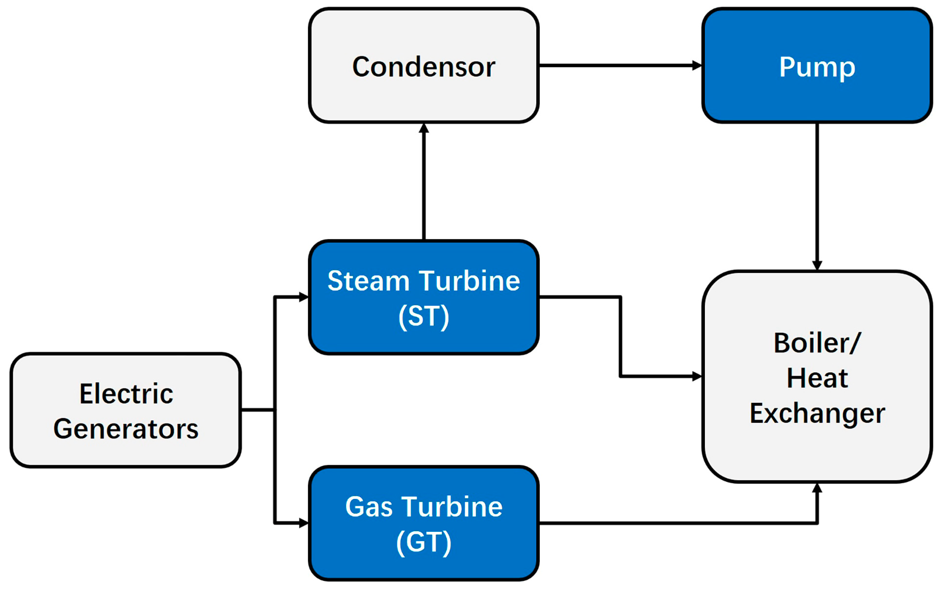
A CCPP system mainly is primarily composed of a gas turbine (GT), steam heat recovery generators (SHRGs), and a steam turbine (ST) [
4]. In a CCPP, a GT produces both hot gases and electrical power (PE). These gases from the GT will then pass over a water-cooled heat exchanger (HE) to generate steam, which can be used to produce PE with the help of the ST in conjunction with coupled generators.
Figure 1 shows a brief workflow of a Combined Cycle Power Plant.
The performance of a power plant operating at full load can be affected by a variety of factors such as ambient temperature, atmospheric pressure, relative humidity, exhaust steam pressure, and so on [
5], which makes it challenging to create a reliable mathematical model for CCPPs. Various techniques have been used to predict power generation, including physical, statistical, and machine learning methods.
The conventional physical methods use numerical weather prediction (NWP) models to simulate atmospheric dynamics based on physical principles and boundary conditions [
6]. However, this type of method requires a high number of input/environment parameters and thermodynamical assumptions to represent the actual system [
7,
8,
9], and may take too much effort and computational resources [
3,
10]. Furthermore, it can not ensure performance when meteorological factors change rapidly or encounter unexpected errors, according to the literature [
11].
Compared with physical prediction models, statistical methods such as the auto regressive moving average [
12], the Bayesian approach [
13], the Kalman filter [
14], the Markov Chain model [
15], and the gray theory [
16] were more widely used. However, most of the existing statistical prediction models are linear models, rendering it difficult to forecast long-term electricity supply [
6].
In recent years, with the development of Artificial Intelligence, machine learning methods have been applied in various computation-intensive domains, such as autonomous driving (AD), natural language processing (NLP), robotics, etc. [
17,
18,
19]. These methods can replace conventional thermodynamical methods and statistical methods to predict the net hourly electrical energy produced by power plants [
20].
Machine learning is a branch of artificial intelligence (AI) that involves developing algorithms and models that enable machines to learn from data and make predictions or decisions based on that learning. The main goal of machine learning is to build models that can automatically identify patterns and relationships within large and complex datasets [
21]. Several studies have been carried out using machine learning techniques to make electricity forecasts.
According to [
20,
22], K nearest neighbors (K-NN), Linear Regression, and RANSAC regressions can achieve better performance than Simple Linear Regression, Bayesian Linear Regression, Decision Tree, and Gaussian Naïve Bayesian Regression algorithms based on the CCPP dataset. K-NN is a type of instance-based learning where new data points are classified or predicted based on their similarity to the training data. However, the predictive outcome of the K-NN algorithm is highly influenced by the selection of the value of K. A smaller K value tends to result in a more flexible model that is prone to overfitting, while a larger K value often leads to a more rigid model that may suffer from underfitting. Linear regression is a statistical technique that is commonly employed to model the correlation between a dependent variable and one or multiple independent variables. Rabby Shuvo et al. [
23] employed four distinct machine learning regression techniques to make predictions for the hourly overall energy production of CCPPs. Their study demonstrates that the linear regression model outperforms the random forest, Lasso regression, and decision tree. However, the linear regression algorithm also has some limitations and drawbacks. Linear regression algorithms assume a linear relationship between the dependent variable and the independent variable(s). However, in many real-world situations, including in the CCPP dataset, the relationship may not be linear, and nonlinear regression techniques may be more appropriate. As for RANSAC (RANdom SAmple Consensus) regression, it assumes that the errors in the model are normally distributed and maintain uniform variance. This assumption may not hold true for the CCPP dataset.
Support vector regression (SVR) is a machine learning technique that is commonly used for regression analysis. Fan et al. [
24] presented a combination blended model of support vector regression, differential empirical mode decomposition, and autoregression techniques to predict electric load. Malvoni et al. [
25] proposed a Least Squares Support Vector Machine (LS-SVM) for photovoltaic power forecasting. Then, Afzal et al. [
10] developed an SVR (RBF) model hybridized with a Ridge cross-validated (RidgeCV) algorithm to predict the output of CCPPs and achieved 0.92 R
2. According to [
26], SVR presents notable benefits for addressing regression-related problems, especially with small dataset sizes. However, it may encounter computational challenges when applied to large datasets. In addition, SVR is highly sensitive to its internal parameters. Furthermore, incorrect parameter selection may result in a considerable decrease in prediction accuracy.
Tree-based algorithms have also been applied to this research topic. According to [
22,
27], Decision Tree (DT), Gradient-Boosted Regression Tree (GBRT), and Bootstrap-Aggregated Tree algorithms could achieve extremely outstanding performance after performing certain preprocessing on the dataset. Furthermore, Prabhas and Rouzbeh [
28] used Random Forest Regression (RFR) to predict the power output after using Z-score normalization to standardize the dataset. Their predicted results were then destandardized using the same mean and standard deviation from the training set, and they achieved a better result (R
2 = 95.9%) than Linear Regression, Multilayer Perceptron, and Support Vector Regression. However, these tree-based algorithms can easily overfit the data, especially when the tree is deep and has many branches. This can lead to poor performance on new, unseen data. Furthermore, these methods are inadequate for capturing linear relationships between variables because they only split the data based on discrete thresholds.
Recently, deep learning (DL) has made significant success in various domains, including image recognition, natural language processing, speech recognition, and resource management [
29,
30]. Deep neural network (DNN) is a multilayer neural network that can utilize the output features of the preceding layer as input for the succeeding layer. By iteratively mapping the features of input samples from their original space to a new feature space layer by layer, DNNs could improve the quality of feature representation for the given input data and could have a better representation of the input data in a transformed feature space. The application of DL in the power system has become a hot research topic. It has the potential to enable more efficient and accurate prediction and diagnosis, thereby enhancing the stability and economy of the power grid. Rashid et al. [
31] proposed a Particle Swarm Optimization Trained Feed-Forward Neural Network to predict the energy of the power generation system and achieved 0.0055 mean square error (MSE) for the testing data, but their inputs and output had been normalized in a range of [0, 1]. Wang et al. [
32] used an ensemble of deep learning-based approaches for efficient forecasting of wind power. Furthermore, Prabhas and Rouzbeh [
28] built an MLP with one hidden layer and Rectifying Linear Unit (ReLU) activation function and achieved MAE = 3.2, RMSE = 4.2, and R
2 = 93.8 based on the CCPP dataset. Akdemir [
7] used the Artificial Neural Network to manage CCPP and obtain the predictable energy output with the RMSE (4.32) after two-fold cross-validation. However, ANNs are prone to overfitting and can easily get trapped in local minima [
33]. Furthermore, ANNs have numerous hyperparameters that need to be tuned to optimize model performance. Identifying the optimal values of these hyperparameters is a formidable task because they are highly dependent on the specific problem and dataset.
In 2017, Ashish et al. [
34] presented the Transformer mechanism to solve machine translation tasks. The network structure of the Transformer is entirely composed of self-attention and Feed-Forward networks. This structure is particularly important in natural language processing, where words in a sentence are not only related to their context but also have varying degrees of relevance to other words in the context. Later, the Transformer mechanism was applied in many other fields and achieved good performances due to its ability to facilitate the modeling of extended dependencies between input sequence elements and enable parallel processing of sequences, as compared to recurrent networks [
35]. Considering that DNNs are capable of mapping inputs to high-dimensional spaces and the Transformer encoder could allow the network to focus on the more important features and data patterns from the high-dimensional space, combining DNN with Transformer mechanisms could be a possible solution to predict the power generation from a CCPP.
4. Methodology
In our proposed model, we have combined Transformer encoders with a DNN. To enhance the DNN component, we have implemented some modifications by replacing the DNN with a sequence of bottleneck DNN blocks. Furthermore, these bottleneck blocks are interconnected via residual connections.
4.1. Transformer Encoders with DNN
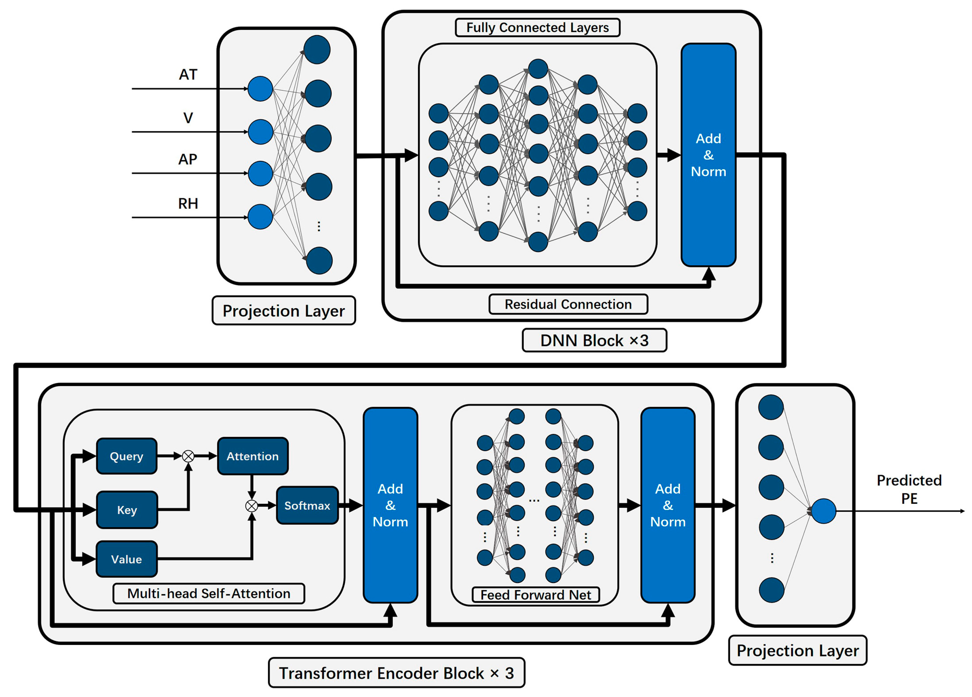
DNNs are capable of mapping inputs to high-dimensional spaces through multi-layer linear combinations, with each layer followed by a Leaky Rectified Linear Unit (LeakyReLU) activation function, so DNNs could make features more complex and nonlinear, leading to a richer representation. In addition, the self-attention mechanism in the Transformer encoder allows the network to focus on the more important features and data patterns in the high-dimensional space. We propose a model that combines DNN blocks and Transformer encoders, taking AT, V, AP, and RH as inputs, passing through DNN layers, and then through Transformer encoders, to obtain the predicted value of PE.
The structure of the proposed model is shown as follows:
As shown in
Figure 5, four input features (after data standardization) first pass through a projection layer and are mapped to high-dimensional space. Then, they enter three DNN blocks and then three Transformer encoder blocks sequentially. At last, data flow into a projection layer to output the predicted PE value.
In Transformer encoder blocks, data first pass through a multihead self-attention module. Different from the usual input format of Transformer, samples in the CCPP dataset are single-step. In this case, it can be considered that multi-head self-attention plays a role in dividing the high-dimensional space into several different subspaces (the number of subspaces is determined by the number of attention heads). By computing attention scores between these subspaces, the network can identify correlations and patterns within the data across different subspaces, enabling it to focus on the most important statistical regularities.
Once the data exit the multihead self-attention module, they proceed to the Feed-Forward Net (FFN) module. The FFN module merges the output features from self-attention modules in a linear fashion to achieve a more intricate representation. In a standard FFN module, each layer of the network is followed by an activation function LeakyReLU, and experiments have shown that this nonlinear design could bring better performance.
In our experiments, we used AdamW as the optimizer and set the learning rate to 1 × 10⁻³ and then trained the network for a total of 200 epochs. Moreover, some training strategies like learning rate decay were applied in the training procedure.
4.2. Bottleneck DNN Blocks
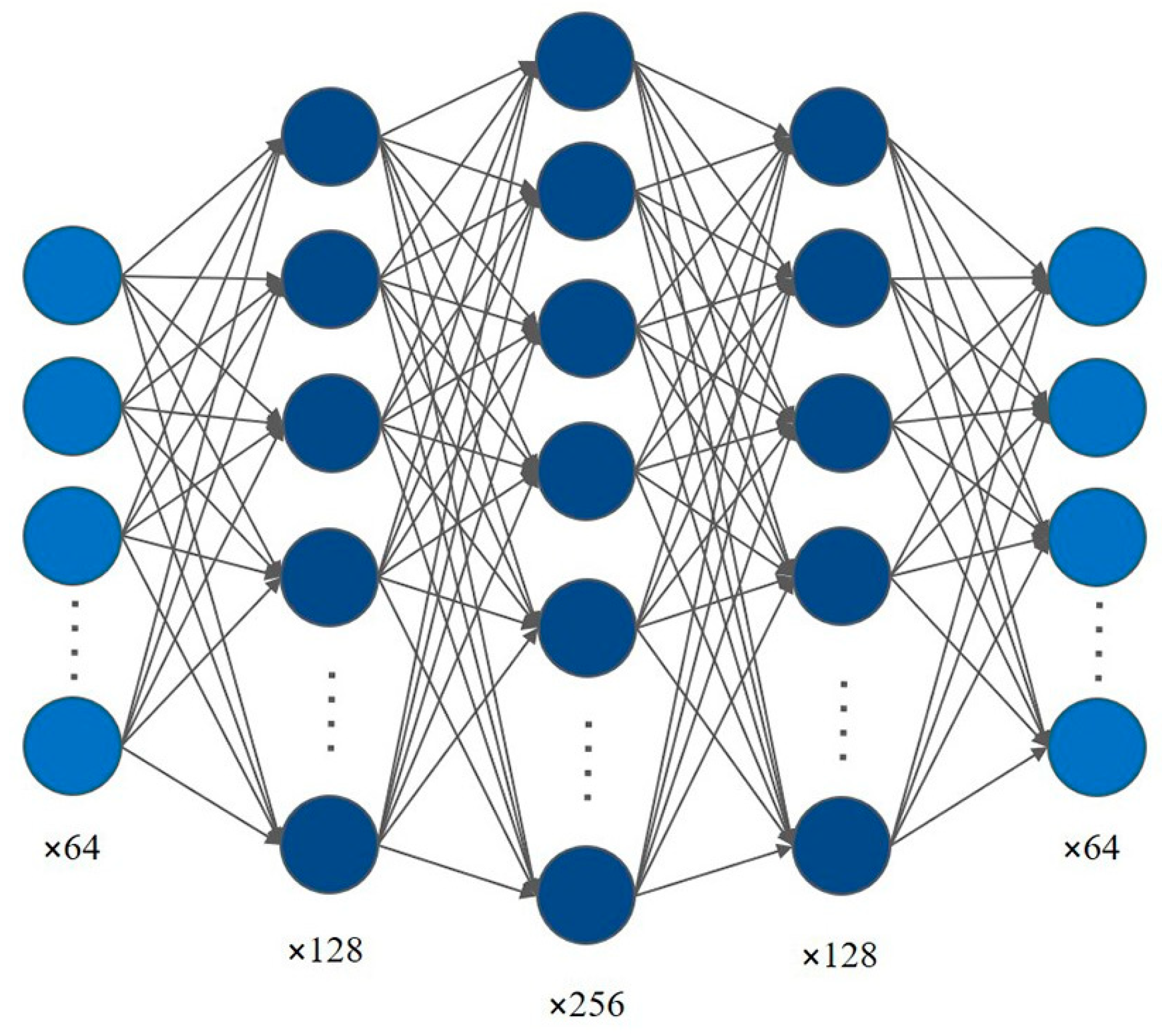
During our experiments, we split the DNN into several blocks, with each block consisting of an internal bottleneck network structure where each layer is composed of 64, 64×2, 64×4, 64×2, and 64 units. When data enter a bottleneck DNN block, they would first be up-dimensioned and then down-dimensioned. Compared with DNNs, which have a consistent number of neurons in each of their hidden layers, the up-dimension operation can combine different types of features to improve the discrimination ability of the DNN model. In addition, the down-dimension operation can remove features with low differentiation degrees. In general, the dimensionality reduction and dimensionality enhancement operations enable the bottleneck DNN to learn more intrinsic useful features and exclude the interference of useless features. The structure of a bottleneck DNN block is shown as in
Figure 6:
Furthermore, for a given network depth, a DNN constructed with bottleneck blocks could have a smaller number of parameters and be more scalable than traditional DNNs, indicating that the DNN composed of bottleneck blocks is relatively easier to train and modify its overall network size.
4.3. Residual Connections between Bottleneck DNN Blocks
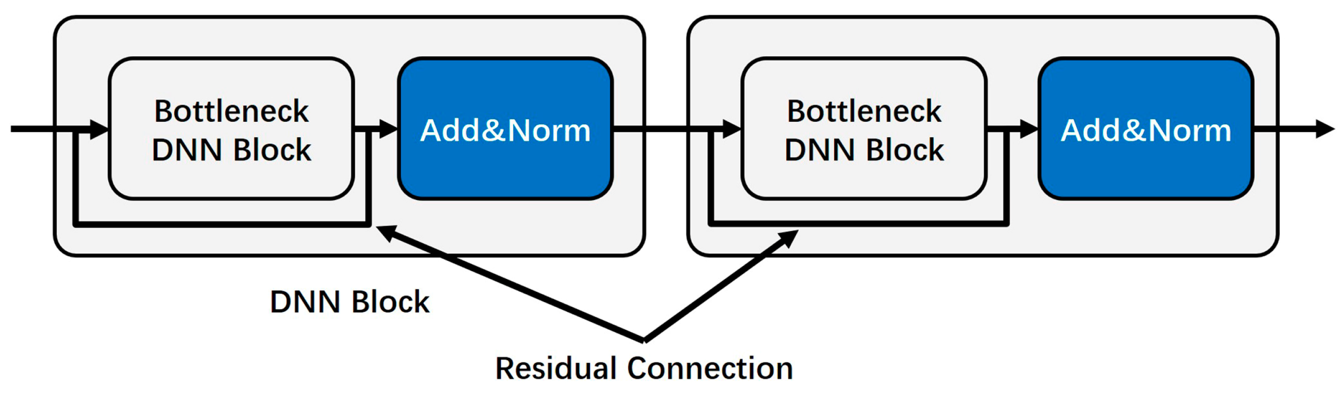
Deep neural networks are usually difficult to train and prone to network degradation. The emergence of residual connections can effectively solve this problem. In our proposed model, we applied residual connections to combine different bottleneck DNN blocks. The whole DNN is designed as in
Figure 7:
Moreover, considering that increasing the depth of a network can lead to issues such as gradients vanishing, gradients exploding, and network degradation, residual connections have been integrated into both DNN blocks and Transformer encoders. The inclusion of residual connections also contributes to a more stable training process.
5. Experimental Results and Discussion
5.1. Evaluation Metrics
To evaluate the performance of our proposed model, the results will be evaluated using the following four evaluation metrics:
where,
,
and
separately denote original, predicted PE data, and the average of PE data, respectively.
For the three metrics of RMSE, MAE, and MAPE, a lower value suggests a smaller difference between the predicted and actual PE data, indicating the better predictive performance of the model. As for the R2, its value falls within the range of [0, 1]. With the R2 approaching 1, it implies that the model has a better ability to fit the data.
5.2. Machine Learning Algorithms and Parameter Selection
In this paper, six traditional machine learning algorithms are used to predict the PE data, including K-nearest neighbor (KNN), linear regression (LR), support vector regression (SVR), decision tree (DT), random forest (RF), and gradient boosting (GB). In addition, multilayer perceptron (MLP) and deep neural network (DNN) have also been applied for prediction as a comparison to the proposed model Transformer Encoders with DNN.
During our experiments, we selected Scikit-learn to implement the above-mentioned six machine learning algorithms and MLP algorithm for prediction on the CCPP dataset.
For K-NN, we empirically selected the values of K from the set of the odd number ranging from 3 to 15, and the algorithm showed the best performance when K is set to 5.
For SVR, the kernel function has been set successfully as linear, poly, sigmoid, and radial basis function (RBF). The results show that the RBF could best exploit the algorithm.
For Decision Tree, we selected the values of max depth ranging from 5 to 15, and when it is set to 10, the algorithm gives out the best performance.
For Random Forest, we referred to the selection of hyperparameters from [
3].
For Gradient Boosting, the values of n_estimators have been set to 250, 275, 300, 325, 350, 375, and 400. The MAE drops from 2.6452 (n_estimator is set to 350) to 2.6032 (n_estimator is set to 400), indicating that when the n_estimator is set to after 350, the improvements are not significant. To strike a balance between accuracy, computation complexity and overfitting, we ultimately set the n_estimator to 400 in our experiments.
For MLP, there are four hidden layers, each composed of 128 units, and the max_iter is set to 1000.
For the rest of the methods, we use the default parameters to conduct the experiments.
5.3. Comparison of DNNs and Bottleneck DNNs
To evaluate the performance of bottleneck DNNs, we constructed DNNs with different structures to perform the prediction of PE values on the CCPP dataset. The hyperparameters of different DNN structures and their performances on the dataset are shown in
Table 2:
For all the DNN models listed in
Table 2, the selected activation function is LeakyReLU. As shown in
Table 2, we set a certain network depth (five or nine) and aligned the DNNs and bottleneck DNNs at the widest layer. The results indicate that bottleneck DNNs can achieve better performance in terms of the four selected evaluation metrics. Furthermore, bottleneck DNNs have a smaller number of parameters than DNNs, which indicates a faster training procedure. Hence, we chose the bottleneck DNN structure for our proposed method.
5.4. Results
All the experiments are performed on Intel(R) Core(TM) i7-9750H CPU 2.60 GHz and NVIDIA GeForce GTX 1660 Ti.
After processing the CCPP dataset, six machine learning algorithms were conducted to predict the PE data for comparison experiments. In addition, MLP, DNN, and Transformer encoders with DNN models were constructed for prediction. The experimental results indicate that the proposed model is more effective than the other models mentioned, with the root mean square error (RMSE) = 3.5370, the mean absolute error (MAE) = 2.4033, the mean absolute percentage error (MAPE) = 0.5307%, and the R
2 = 0.9555. The complete prediction error evaluation metrics are shown in
Table 3:
5.5. Discussions
We compared the predictive results of our proposed model with those of other algorithms. As shown in
Table 3, the predictive results of Transformer encoders with DNN are better than the other models in terms of those evaluation metrics RMSE, MAE, MAPE, and R
2.
From an algorithmic perspective, the main reason why our proposed model performs better than the others can be summarized as follows:
Four inputs of CCPP data are mapped to a high-dimension space through a projection layer. Inside the DNN blocks, linear transformations are conducted in the forward propagation so that different types of features are combined. Furthermore, considering that the activation function is LeakyReLU, from which linear features can be transferred to nonlinear features, this enhances the network’s ability to express itself and capture more complex features. The output of DNN is then fed into the Transformer encoders, where the self-attention module drives the network to focus more on the underlying data patterns. This helps the network extract more profound and abstract features from the data and predict the results with greater accuracy.
Multihead self-attention is usually used to capture the correlation between different tokens in a sequence. However, considering that all samples in the CCPP dataset are single-step, we observed that multihead self-attention operates by dividing the high-dimensional space into multiple subspaces, in our experimentation. Subsequently, the features within these subspaces undergo separate linear transformations to calculate the attention score. This technique uncovers the inherent relationships in various aspects of the data.
In addition to the aforementioned benefits, the residual connections have been implemented to facilitate the discovery of a more optimal solution for data fitting. Since the stochastic gradient descent strategy is used in the training process, the solution obtained is often the local optimal solution rather than the global one, and since the structure of the deep network is deeper and broader, it is more likely that the gradient descent algorithm will get the local optimal solution, leading to the network degradation. Therefore, the residual connection module within the Transformer encoder and between DNN blocks connects the input directly to the subsequent layers through a shortcut without increasing the computational complexity. This mechanism enables the subsequent layers to learn the residuals directly and could partially resolve the information loss induced by fully connected layers during information transfer. As a result, based on the residual connections, we can train a deeper network and achieve better predicting performance.
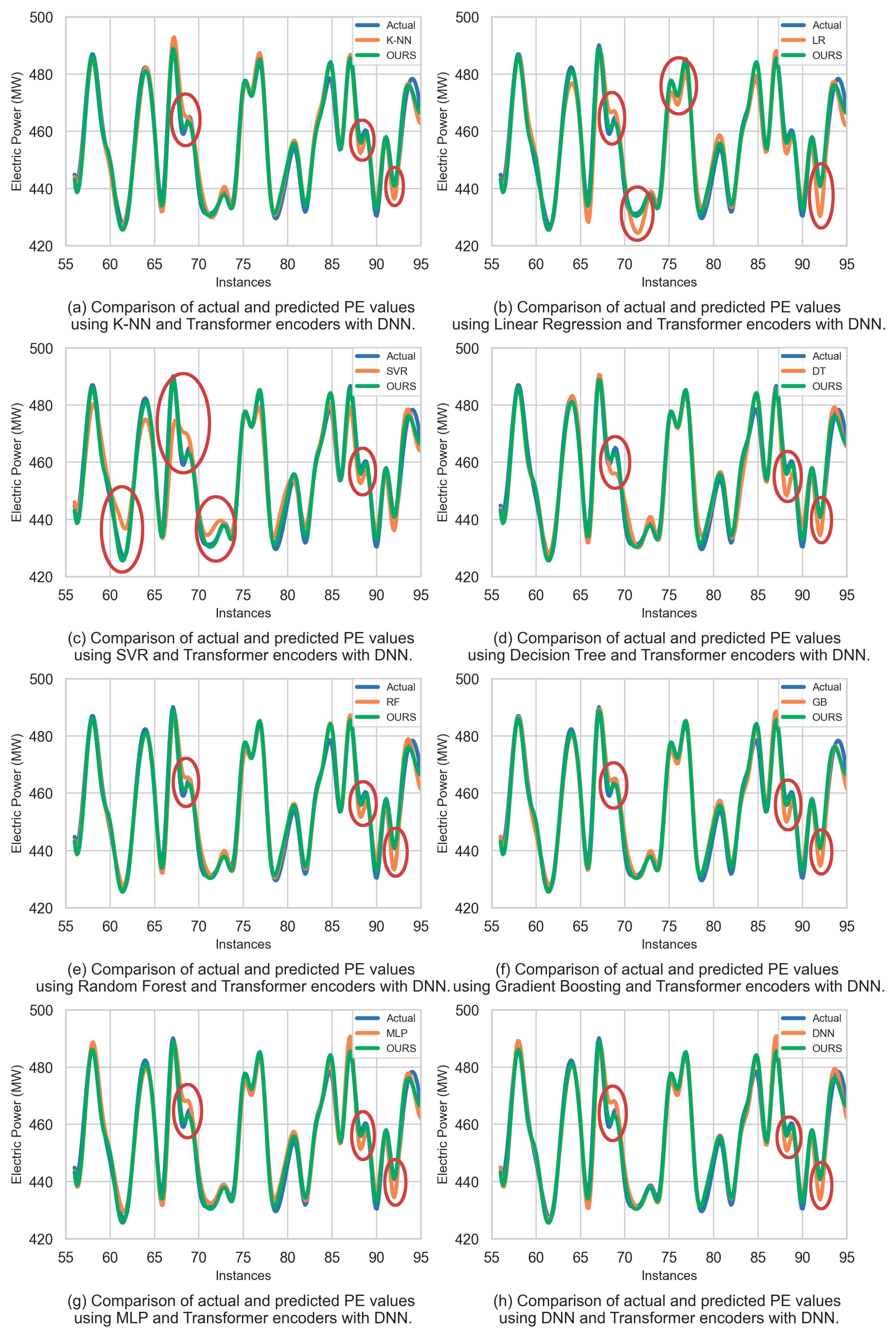
As shown in
Figure 8, we selected 40 samples from the testing set to compare the actual PE value with the predicted PE value using our proposed model and the other eight methods. We observed that machine learning models are less sensitive to data that tend to change abruptly, and neural networks apparently have better adaptability to trace the trend. Moreover, the proposed method performs better when it comes to approaching the actual value than the other methods in terms of prediction of the extreme and minimal values. Compared with MLP, DNN, or ensemble learning models, such as random forest and gradient boosting, our proposed model is more apt to capture more slight oscillation and thus fit the data more accurately.
6. Conclusions and Future Work
This study employs the publicly accessible CCPP dataset to predict power output, which includes four independent input parameters, ambient temperature, atmospheric pressure, relative humidity, and vacuum. The performances of six traditional machine learning algorithms, MLP, and DNN were evaluated as competitive experiments. Following that, we employed Transformer encoders with DNN to conduct the predictions. Firstly, we split the DNN into three blocks, each consisting of a bottleneck structure where data is first up-dimensioned and then down-dimensioned. Secondly, these bottleneck DNN blocks are interconnected to each other using residual connections. Thirdly, DNN and Transformer encoders are combined. The results show that our proposed model outperforms other machine learning approaches in terms of prediction accuracy, with RMSE = 3.5370, MAE = 2.4033, MAPE = 0.5307%, and R2 = 0.9555. The following stands are K-Nearest Neighbors, Linear Regression, Support Vector Regression, Decision Tree, Random Forest, Gradient Boosting, Multilayer Perceptron, and Deep Neural Networks models. This demonstrates that our proposed algorithms are suitable for modeling the energy output of the CCPP based on thermal input parameters.
Nevertheless, the proposed model has some internal weaknesses for us to overcome in the future. Considering that deep neural networks are prone to overfitting, the selection of hyperparameters requires elaborate experiments to reach its best effectiveness. Furthermore, as the network’s overall scale increases, the training process becomes more time-consuming. For future work, from the perspective of data preprocessing, additional advancements can be made by focusing on further feature engineering to enhance prediction accuracy. Furthermore, from an algorithmic standpoint, further investigations can be conducted to optimize the network’s structure. Various optimization algorithms, such as genetic algorithms and Ant Colony Optimization (ACO) algorithms, could be employed to optimize the neural network’s parameters. Additionally, we plan to apply the proposed model to a broader range of electricity power scenarios, including the power prediction of different types of power plants and electricity load prediction. More features collected by sensors that may affect the power output could be fed into the model to achieve better accuracy. Furthermore, the proposed model can also be taken into consideration in terms of regression application.


