Channel Estimation for High-Speed Railway Wireless Communications: A Generative Adversarial Network Approach

Abstract

In high-speed railways, the wireless channel and network topology change rapidly due to the high-speed movement of trains and the constant change of the location of communication equipment. The topology is affected by channel noise, making accurate channel estimation more difficult. Therefore, the way to obtain accurate channel state information (CSI) is the greatest challenge. In this paper, a two-stage channel-estimation method based on generative adversarial networks (cGAN) is proposed for MIMO-OFDM systems in high-mobility scenarios. The complex channel matrix is treated as an image, and the cGAN is trained against it to generate a more realistic channel image. In addition, the noise2noise (N2N) algorithm is used to denoise the pilot signal received by the base station to improve the estimation quality. Simulation experiments have shown the proposed N2N-cGAN algorithm has better robustness. In particular, the N2N-cGAN algorithm can be adapted to the case of fewer pilot sequences.

1. Introduction

The high-speed railway (HSR) has gradually become one of the most preferred ways for people to travel, because of its convenience, flexibility, and high speed. To better meet passengers’ expectations of a high-quality experience and safe train operation control, the performance demand of communication systems is increasing [1]. The development of creative communication network designs is essential for the rail transit sector. In the typical scenario of fifth-generation mobile communication technology (5G) [2], the HSR scenario targets its high data rate, low delay, and low energy consumption. Under the 5G communication system [3], HSR is designed to provide data transfer rates of 150 Mbps when a mobile speed of up to 500 km/h or higher.

However, HSR scenarios are typical scenarios with continuous wide-area coverage and high mobility [4], so the characteristics of wireless channels are quite different from those in conventional scenarios. For example, due to the fast mobility and complex terrain [5,6], there are Doppler effects in the information transmission process, rapid changes in small-scale fading, and short coherence times. The channel is fast time-varying. These special characteristics make the design of the transmission algorithm of the system more challenging [7]. In particular, the high-precision channel estimation is more difficult. Therefore, the research of channel estimation in HSR scenarios is an important and challenging technical field [8].

Moreover, massive multiple-input multiple-output (MIMO) [9,10] systems are widely recognized as the foundational elements of 5G technology [11]. Deploying large-scale antenna arrays at base stations (BS) can greatly improve network capacity and user experience. However, the massive MIMO itself is a technical problem for channel estimation, because it will increase computational complexity. Therefore, the way by which to design a channel estimation algorithm with low computational complexity and simultaneously fit its own architectural features is an issue for a 5G HSR communication system. Traditional channel estimation algorithms cannot effectively solve the above problems.

Generally, traditional channel estimation includes blind channel-estimation methods [12] and pilot-assisted channel-estimation methods [13]. For blind channel-estimation methods to count the correlation properties of the channel, a great deal of data is needed, which will lead to slow convergence and high complexity of the algorithm [14]. In high-mobility environments, blind channel-estimation methods are generally considered infeasible. The reason is that blind channel-estimation methods need to keep the channel characteristics constant in the analysis, while in a high-mobility environment, such as HSR scenarios, the channel will change rapidly in a short time. The pilot-assisted estimation methods need to add auxiliary data to the transmitter, so it will occupy the sending resources of the transmitter. The pilot-assisted estimation methods are usually performed by using algorithms such as least square (LS) [15] and linear minimum mean square error (LMMSE) to estimate the CSI in the frequency domain at the pilot frequency symbols [16,17,18]. The channel frequency response (CFR), however, is often assumed by these approaches to fluctuate linearly. High-speed movement of the terminals will introduce a Doppler effect in HSR scenarios, which causes the CFR to change rapidly. At the same time, the Doppler effect will seriously affect the effectiveness of the estimation algorithm and lead to the degradation of the estimation performance. Therefore, in order to ensure extreme user experience (100 Mbit/s) and safe train operation control for the 5G HSR communication systems, channel-estimation technology that adapts to fast time-varying channels and massive MIMO systems should be paid more attention.

The development of deep learning (DL) technology has led to satisfactory results in the field of communication [19]. It has shown excellent performace in signal detection [20], channel coding [21], signal classification [22], and CSI feedback [23]. Some researchers also apply DL to channel estimation. One type is the direct use of neural networks to learn the various characteristics of the channel and then estimate the complete CSI from the pilot sequence signal. In [24], the approaches for massive MIMO systems forecast channels much more accurately than conventional channel-estimation algorithms. In [25], a deep neural network-based online estimation method is adopted for dual selective fading channels. A channel-estimation method based on DL in the high mobile environment is proposed and the maximum pooling network is used to reduce the dimension of the parameters in [26]. In [27,28], a neural network channel-estimation optimizer based on the MIMO-OFDM system to optimize the LS algorithm was proposed. The other type is to treat the CSI as an image and use image-processing techniques to recover the channel. In [29], the idea of treating the channel matrix as a two-dimensional (2D) natural image and combining it with image-reconstruction techniques for channel estimation is proposed for the first time. In [30], a wideband channel-estimation method based on a generation countermeasure network (GAN) is proposed. Furthermore, it is noted that the estimator based on GAN can lower the necessary pilot’s requirement without noticeably raising the error and necessary signal-to-noise-ratio (SNR). In [31], conditional GAN (cGAN) is used as channel estimation, where the generator estimates the channel from the pilot signal received by the BS. Although the aforementioned research uses deep learning to address channel-estimation issues in a variety of communication systems, it does not adequately account for the effects of rapidly changing surroundings on large MIMO systems [32].

Additionally, it is worth noting that environmental noise is a critical factor that can significantly impact the quality of channel estimation. Therefore, for denoising channel estimation algorithms, the pilot signals at the receivers before estimation can also improve the estimation quality [33]. Due to the convolutional neural network (CNN)’s strong performance in image-recognition and processing tasks, more and more studies have applied CNN-based image denoising algorithms to design channel-estimation methods. In this kind of research, the receiver’s channel matrix and pilot matrix are frequently seen as images. More specifically, an image can be represented by a complex number of real and imaginary parts, respectively. In [34], supervised learning is utilized in denoising CNN (DnCNN), which involves learning the residual noise from noisy channels. Then, to get residual noise, the channel generated from the rough estimate is fed into the trained DnCNN. Finally, the rough estimation channel is subtracted from the residual noise to obtain more accurate estimation results. Similar to how it was used to analyze the rough estimates of the channel to get a more precise estimation, DnCNN is also employed as the denoising network in [35].

To enhance the channel estimation accuracy in the high-speed railway (HSR) environment of massive MIMO systems, we propose a N2N-cGAN channel-estimation algorithm that combines the WINNER II D2a channel model [36] with image-denoising technology. In N2N-cGAN, both the denoising network and the generator network adopt the U-Net network structure, which can effectively capture and utilize the spatial dependencies in the input data to better meet the requirements of channel-estimation tasks. The discriminator uses a CNN and a patch architecture to distinguish between the input real channel information and the generated channel information. Specifically, we consider a predenoising channel estimation strategy for channel estimation. The channel-estimation process has two stages. In the first stage, the pilot signal is treated as an image, and a novel image denoising method, N2N [37] is proposed. Unlike traditional denoising methods, N2N does not require an accurate noise model or a clean reference image. It achieves high-quality denoising by learning the general ability to remove noise from multiple noise samples during training, with strong robustness and versatility. In the second stage, we use cGAN to estimate the channel. Compared with other traditional methods, this cGAN-based channel-estimation method can better utilize the characteristics and structure of channel estimation data, thereby improving estimation accuracy. Due to the parallel nature of these two stages, the training speed can be significantly accelerated. The contributions of this paper can be summarized as follows.

• The N2N algorithm does not need a noiseless signal as a training target. Moreover, the outcomes are more manageable because it is end-to-end training. Therefore, in order to reduce the error of channel estimation, the received pilot signal is denoised by using the N2N method before channel estimation.
• The cGAN structure’s GAN loss improves the neural network’s optimization [38], thereby enabling our channel-estimation method to perform well even in low SNR conditions.
• Numerous simulation results demonstrate how our proposed algorithm may successfully lower the channel estimate error and improve system performance in HSR circumstances, even with very short pilot sequence sequences.

The rest of this paper is organized as follows: Section 2 presents system and channel model. Section 3 presents the proposed N2N-cGAN-based channel-estimation algorithm. Simulation results are provided in Section 4, and conclusions are shown in Section 5.

2. System and Channel Models

2.1. System Model

The typical wireless communication systems on HSR are shown in Figure 1. The BSs are situated alongside the railway, covering the communication within a community. The relay station (RS) is installed at the top of the carriage to communicate with BS and the user equipment on the train. Here, we design the wireless communication that RS sends data symbols to BS and consider a MIMO-OFDM system with $N_T$ transmitting antennae and $N_R$ receiving antennae. Suppose there are N subcarriers and T OFDM symbols in a subframe. Data symbols encounter reflection, refraction, and diffraction caused by scatterers during transmission. However, there are strong line of sight (LOS) components in space.

In Figure 1, $c\left(0\right),c\left(1\right),\dots ,c(L-1)$ denotes the frequency selection channel, and L is the number of the frequency selection channel. The formula for calculating the Doppler frequency shift is

$$f_d=\frac{v}{c}{f}_{c}cos\theta ,$$

(1)

where c represents the speed of light, $c=3\times {10}^8$ m/s, $\theta$ is the angle of arrival of the LOS component.

For example, high-speed trains can reach speeds of up to 360 km/h on conventional routes. Assuming that the carrier frequency $f_c$ is 3.5 GHz, the maximum Doppler frequency shift of the train antenna is

$$f_d=f_c·\frac{v}{c}\approx 1167\mathrm{Hz}.$$

(2)

According to the calculation formula of coherent time, we can get the coherent time $T_S=1/\left(4f_d\right)\approx 0.214$ ms. According to the current 5G-NR standard subcarrier spacing set to 15 kHz, the duration of an OFDM symbol is 0.0667 ms. Coherent time $T_S$ is the duration of more than one OFDM symbol. Therefore, we can assume that the multipath channel in an OFDM symbol is time-invariant, but the channel changes in different symbols.

At the transmitter, the transmitting signal obtained after space–time coding and serial/parallel conversion can be expressed as $X_{N_t}$, where $X_{N_{\mathrm{t}}}=\left[X_{N_{\mathrm{t}}}\left(0\right),\dots ,X_{N_t}\left(k\right),\dots ,X_{N_t}\right.\left.\left(N-1\right)\right]$, $X_{N_{\mathrm{t}}}\left(k\right)$ represents the kth subcarrier of the OFDM symbol on the $N_t$th transmitting antenna. Therefore, the OFDM symbols transmitted by all transmitting antennae can be expressed as

$$\mathbf{X}={\left[{\mathbf{X}}_1,\dots ,{\mathbf{X}}_{{\mathrm{N}}_{\mathrm{t}}},\dots ,{\mathbf{X}}_{{\mathrm{N}}_{\mathrm{T}}}\right]}^{\mathrm{T}}.$$

(3)

After performing IFFT on the data on each transmit antenna, the time domain-modulated signal of the $N_t$th transmit antenna can be expressed as ${\mathbf{x}}_{{\mathrm{N}}_t}$, where

$${\mathbf{x}}_{{\mathrm{N}}_t}={\left[{\mathbf{x}}_{{\mathrm{N}}_t}\left(0\right),\dots ,{\mathbf{x}}_{{\mathrm{N}}_t}\left(k\right),\dots ,{\mathbf{x}}_{{\mathrm{N}}_t}(N-1)\right]}^{\mathrm{T}},$$

(4)

and its matrix form can be expressed as

$${\mathbf{x}}_{N_t}={\mathbf{F}}^{\mathrm{H}}{\mathbf{X}}_{{\mathrm{N}}_t}.$$

(5)

After further processing, the OFDM symbol on the $N_t$th transmit antenna passes through the wireless fading channel. The signal, after being received by the $N_r$th antenna at the receiver, can be expressed as

$${\mathbf{y}}_{N_r}\left(m\right)=\sum _{N_t=1}^{N_T}\sum _{i=0}^{\mathrm{L}-1}{\mathbf{h}}_{N_r,{\mathbf{N}}_t}(m,i){\mathbf{x}}_{{\mathrm{N}}_{\mathrm{t}}}(m-i)+{\mathbf{n}}_{{\mathrm{N}}_{\mathrm{r}}}\left(m\right),$$

(6)

where ${\mathbf{h}}_{N_r,N_t}(m,i)$ represents the channel impulse response of the $N_t$th transmitting antenna and $N_r$th receiving antenna in the ith path. The channels remain unchanged within at least one OFDM symbol, L represents the number of distinguishable paths, and ${\mathbf{n}}_{{\mathrm{N}}_{\mathrm{r}}}\left(m\right)$ represents the additive white Gaussian noise (AWGN) of the $N_r$th receiving antenna. After the time domain-received signal is transformed by FFT, the frequency domain received signal ${\mathbf{Y}}_{{\mathbf{N}}_{\mathbf{r}}}\left(k\right)$ can be obtained as

$${\mathbf{Y}}_{N_{\mathrm{r}}}\left(k\right)=FFT\left\{{\mathbf{y}}_{{\mathrm{N}}_{\mathrm{r}}}\left(m\right)\right\}=\sum _{{\mathrm{N}}_{\mathrm{t}}=1}^{{\mathrm{N}}_{\mathrm{T}}}{\mathbf{H}}_{{\mathrm{N}}_{\mathrm{r}},{\mathrm{N}}_{\mathrm{t}}}\left(k\right){\mathbf{X}}_{{\mathrm{N}}_{\mathrm{t}}}\left(k\right)+{\mathbf{N}}_{N_{\mathrm{r}}}\left(k\right),$$

(7)

where ${\mathbf{X}}_{{\mathrm{N}}_{\mathrm{t}}}\left(k\right)$ represents the transmission signal of the transmitting antenna $N_t$th on the kth subcarrier, ${\mathbf{Y}}_{N_{\mathrm{r}}}\left(k\right)$ represents the reception signal of the receiving antenna $N_r$th on the kth subcarrier, ${\mathbf{N}}_{N_{\mathrm{r}}}\left(k\right)$ represents AWGN, and ${\mathbf{H}}_{{\mathrm{N}}_{\mathrm{r}},{\mathrm{N}}_{\mathrm{t}}}\left(k\right)$ represents the channel frequency domain response of the transmitting antenna $N_t$th and the receiving antenna $N_r$th on the kth subcarrier. Therefore, all received signals can be expressed as

$$\mathbf{Y}=\mathbf{HX}+\mathbf{N},$$

(8)

where $\mathbf{Y}={\left[{\mathbf{Y}}_1,\dots ,{\mathbf{Y}}_{N_R}\right]}^{\mathbf{T}}$, ${\mathbf{Y}}_n={\left[{\mathbf{Y}}_{\mathbf{n}}\left(0\right),\dots ,{\mathbf{Y}}_{\mathbf{n}}\left(N-1\right)\right]}^{\mathbf{T}}$ represents the received signal of the nth receiving antenna, $\mathbf{N}={\left[{\mathbf{N}}_1,\dots ,{\mathbf{N}}_{N_R}\right]}^{\mathbf{T}}$, and $\mathbf{N}$ is the corresponding AWGN matrix. $\mathbf{H}$ represents the frequency domain channel matrix, which can be expressed as

$$\mathbf{H}=\left[\begin{array}{cccc}{\mathbf{H}}_{11}& {\mathbf{H}}_{12}& \cdots & {\mathbf{H}}_{1N_T}\\ {\mathbf{H}}_{21}& {\mathbf{H}}_{22}& \cdots & {\mathbf{H}}_{2N_T}\\ ⋮& ⋮& \ddots & ⋮\\ {\mathbf{H}}_{N_{R}1}& {\mathbf{H}}_{N_{R}2}& \cdots & {\mathbf{H}}_{N_R{N}_T}\end{array}\right].$$

(9)

2.2. High-Speed Railway Channel Model

High-speed railway channels and conventional public mobile communication channels are distinct from one another [39]. The Doppler shift has a significant impact on mobile channels, particularly in high-speed scenarios. For the HSR wireless channel model, the WINNER II D2a channel model is a suitable choice, where the cluster is used as the basic unit, and each cluster contains 20 reflectors. The rays formed by the signal passing through the reflectors form a clustering signal, The number of clusters varies from 8 to 24 according to the scene, as shown in Figure 2. The nth cluster’s latency ${\tau }_n^{{}^{\prime }}$ obtained from [36] is determined by

$${\tau }_n^{{}^{\prime }}=-r_{\tau }{\sigma }_{\tau }ln\left(X_n\right),$$

(10)

where the cluster’s delay coefficient is $r_{\tau }$, and the delay spread’s root mean square (RMS) is expressed as ${\sigma }_{\tau }$, a random integer from the common normal distribution is $X_{\mathrm{n}}$. In the WINNER II D2a scenario, $r_{\tau }$ and ${\sigma }_{\tau }$ have values of 3.8 ns and 40 ns, respectively. After setting ${\tau }_n^{{}^{\prime }}$ t’s minimum value to zero, they are sorted in ascending order

$${\tau }_n=sort\left({\tau }_n^{{}^{\prime }}-min\left({\tau }_n^{{}^{\prime }}\right)\right).$$

(11)

In the WINNER II D2a scenario, the LOS route always exists, therefore we change the value of ${\tau }_n^{″}$ to

$${\tau }_n^{″}=\frac{{\tau }_n^{}}{0.7705-0.0433k+0.0002k^2+0.000017k^3},$$

(12)

where k is the Rice factor in dB.

Consequently, the WINNER II D2a channel model’s time-varying channel impulse response may be expressed as

$$h\left(t,{\tau }_n^{″}\right)=\sum _{n=1}^L{E}_{Ln}\left(t\right)E_{Sn}\left(t\right)\delta \left(t-{\tau }_n^{″}\right),$$

(13)

where L represents the total number of clusters, while $ELn\left(t\right)$ denotes the large-scale fading coefficient, and $ESn\left(t\right)$ denotes the small-scale fading coefficient. $E_{Ln}\left(t\right)$ can be formulated as follows,

$$E_{Ln}\left(t\right)={10}^{\frac{P\left(t\right)-P_L+G_n}{10}},$$

(14)

where $P\left(\mathrm{t}\right)$ is the power of the transmitted signal in dBm, $P_L$ is the value of path lose in dB, $G_{\mathrm{n}}$ is a random variable in dB with zero mean log-normal distribution with standard deviations. In the WINNER II D2a scenario, the $P_L$ model can be represented as

$$\begin{array}{cc}\hfill & P{}_L=40{log}_{10}\left(d\right)+10.5-18.5{log}_{10}\left(h_{bs}{h}_{ms}\right)+1.5{log}_{10}\left(\frac{f_c}{5}\right),\hfill \end{array}$$

(15)

where d, $h_{bs}$, $h_{ms}$, and $f_c$ denote the distance between the train and the base station, the heights of the base station and user equipment (UE), and the operating frequency, respectively.

The small-scale fading coefficient $E_{Sn}\left(t\right)$ is expressed by the following equation,

$$E_{Sn}\left(t\right)=\sum _{n=1}^L{A}_n{e}^{j{\phi }_n}{e}^{j2\pi f_s\left(t\right)·t·cos\left({\alpha }_n\right)},$$

(16)

where each cluster’s amplitude and starting phase are described by $A_n$ and ${\phi }_n$, respectively. Each cluster’s incidence angle is ${\alpha }_n$, and the Doppler shift is $f_s\left(t\right)$.

We estimate the channel on the BS side through the pilot signal sent by the user. Assuming that U users simultaneously send a pilot sequence of length $N_p$ to the BS, we define $Y_c$ as the pilot signal at the receiver sequence without noise, which is defined as

$${\mathbf{Y}}_{\mathbf{c}}=\mathbf{\Phi }\mathbf{H},$$

(17)

where $\mathbf{\Phi }\in {\mathbb{C}}^{U\times N_p}$ is the pilot matrix, which is made up of pilot sequences transmitted by U users. The case of $N_p<U$ is considered here, so it is impossible to ensure the orthogonality of the pilot matrix row (i.e., whether the pilot sequence sent by the user is pairwise orthogonal ). In addition, each user’s pilot sequences are chosen at random, using simple design criteria. The received signal $\mathbf{Y}\in {\mathbb{C}}^{M\times N_p}$ at the BS is expressed as

$$\mathbf{Y}={\mathbf{Y}}_c+\mathbf{N},$$

(18)

where $\mathbf{N}\in {\mathbb{C}}^{M\times N_p}$ is the noise matrix drawn from a sample of the Gaussian distribution.

The purpose of pilot-based channel estimation is to minimize the discrepancy between the actual channel matrix $\mathbf{H}$ and the estimated channel matrix $\stackrel{\wedge }{\mathbf{H}}$. For simplicity, we will call ${\mathbf{Y}}_{\mathbf{c}}$ the clean pilot sequence and $\mathbf{Y}$ the noisy pilot sequence. In addition, since our channel-estimation method cannot deal with complex variables, in the subsequent description of the algorithm, we transform the complex variables that appear in this section into images. For example, $\mathbf{Y}\in {\mathbb{C}}^{M\times N_p}$ is transformed into an image of size $M\times N_P\times 2$, where the real and imaginary parts of $\mathbf{Y}$ correspond to the real and imaginary parts of the image channels, respectively. Through this transformation, we can use CNN to process these data. The details of the N2N-cGAN channel-estimation method are elaborated upon next.

3. Channel Estimation Based on N2N-cGAN

This section introduces a channel-estimation approach based on N2N-cGAN. First, the main idea is briefly explained. The suggested N2N-cGAN algorithm’s framework is then further detailed. Finally, a network architecture is proposed.

3.1. The Main Idea

The N2N-cGAN algorithm mainly includes two steps: first, the pilot picture that the BS receives is denoised by using the N2N denoising algorithm. Then the pilot image after denoising is used to estimate the channel image based on cGAN network.

3.1.1. N2N Denoising

The relationship between noise and image can be divided into three forms: a represents high-quality image, b represents noisy image, and n represents noise. Image denoising aims to eliminate the noise n from the noisy image $b=a+n$ that degrades the image quality. Traditional denoising algorithms usually train the CNN to model from noisy input image b to clean output image a. However, the N2N method is distinct from most denoising algorithms in this regard. The N2N algorithm simply needs clean images corresponding to noisy images with independent noise to compose training data and then trains CNN to learn how to map one noisy image to another. Obviously, N2N cannot completely learn the mapping connection between noisy pictures because noise n and $n^{\prime }$ are independent of one another. However, the neural network trained on this impossible task can obtain the same denoising effect as the neural network trained by the traditional denoising algorithm using clean images. Therefore, in this case, a clean image is unable to be obtained. N2N only needs a clean image corresponding to a noisy image with independent noise, the neural network training can produce good denoising effects. The N2N denoising algorithm’s optimization goal is

$$\begin{array}{c}\hfill \underset{\theta }{argmin}\sum _{i}L\left(f_{\theta }\left(b_i\right),{\stackrel{\wedge }{b}}_i\right),\end{array}$$

(19)

where $b_i$ and ${\stackrel{\wedge }{b}}_i$ are different noisy images, $f_{\theta }\left(·\right)$ is a parameter $\theta$ mapping function, and $L\left(·\right)$ is the loss function.

3.1.2. cGAN Network

The conventional GAN is an adversarial learning framework used to train a generative model, which involves a generator $G\left(\cdot \right)$ and a discriminator $D\left(\cdot \right)$. To create extremely realistic pictures, the $G\left(\cdot \right)$ is trained to produce samples that are similar to real data, while the $D\left(\cdot \right)$ is trained to differentiate between the real and generated samples. The $G\left(\cdot \right)$ is updated based on the feedback from the $D\left(\cdot \right)$, and the discriminator is updated based on the difference between real and generated data. However, the $G\left(\cdot \right)$ is trained to map random noise to the real data distribution, which can introduce instability and randomness in the generated samples. Therefore, cGAN was proposed. In order to establish the mapping between conditional input and real data, it introduced a conditional variable y. Specifically, in order to direct the data creation process, cGAN incorporates condition variable y in the modeling of the $G\left(\cdot \right)$ and the $D\left(\cdot \right)$. In $G\left(\cdot \right)$, the input to the generator is formed by combining the noise variable z with the conditional information y. In the $D\left(\cdot \right)$, the input is the combination of real data x and conditional information y or the generated data $G\left(z,y\right)$ output by the generator. $D\left(\cdot \right)$ estimates the probability that its input $G\left(z,y\right)$ is a real one, given the dataset. A definition of the cGAN’s objective function is

$$\begin{array}{c}\hfill \underset{G}{min}\underset{D}{max}V\left(D,G\right)={\mathbb{E}}_{x\sim p_{data}}\left[logD\left(x,y\right)\right]+{\mathbb{E}}_{z\sim p_z}\left[log(1-D\left(G(z,y)\right))\right].\end{array}$$

(20)

It is possible to produce data based on the new inputs of z and y after the trained $D\left(\cdot \right)$ is acquired.

3.2. N2N-cGAN-Based Channel Estimation

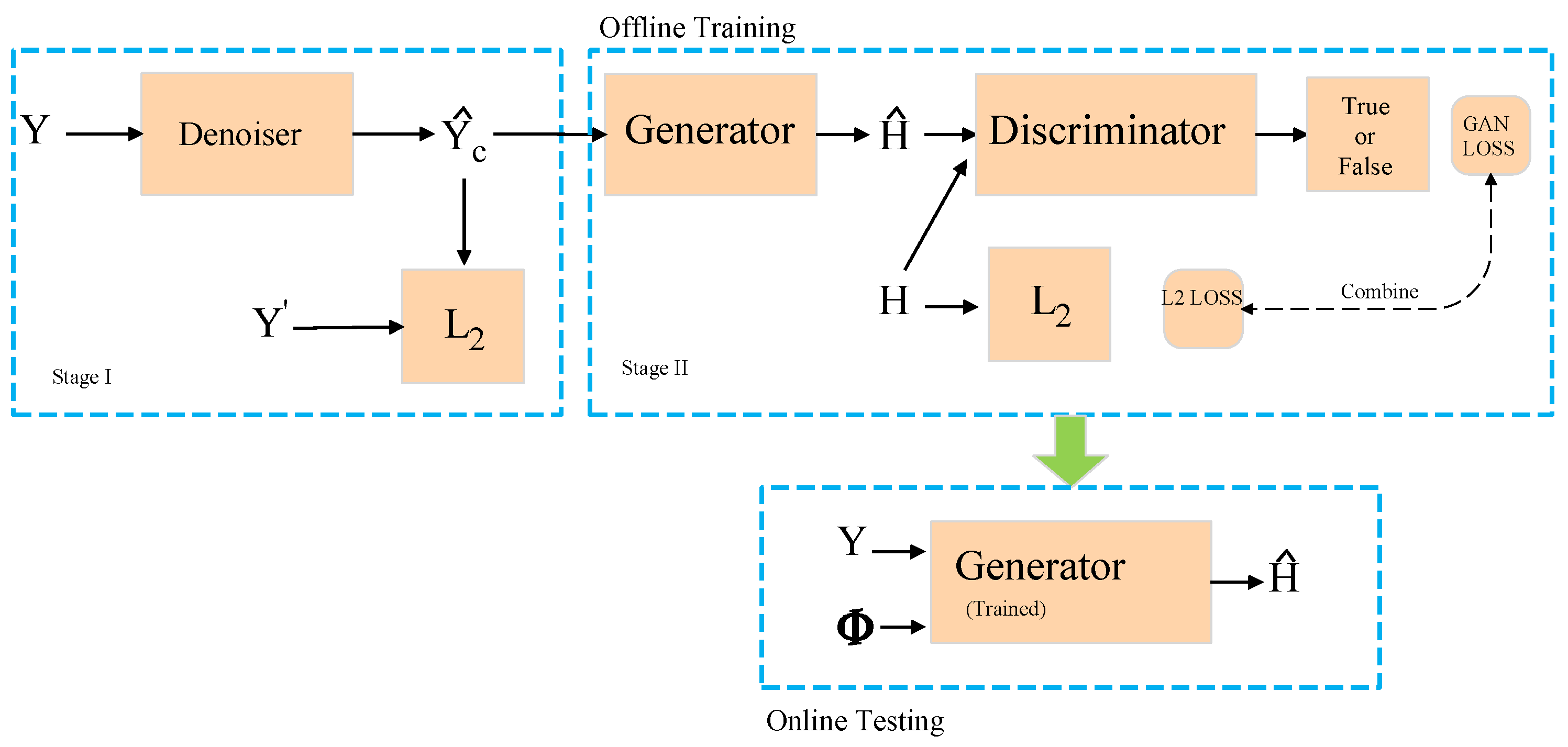
According to Figure 3, the N2N-cGAN channel-estimation process consists of two stages. Stage I sees the denoising device apply the N2N algorithm (i.e., training only using the noisy pilot image.). Since our training dataset contains a portion of the real channel, we can construct a clean pilot signal at the receiver side by using Equation (16). In each round of training for the denoising device, we randomly select a clean pilot image from the training dataset, after which the clean pilot picture is separately sampled, and two AWGNs of equal size are then added. Different signal-to-noise ratios (SNRs) might contribute to the noise power, which can be added to the pilot image to form two noisy pilot images Y and $Y^{\prime }$. In the actual scenarios, the pilot signal can also be sent many times in a coherent time. The pilot signals received by the BS can be regarded as multiple independent noisy versions from the same clean pilot. With two noisy images, Y is input to the denoiser to obtain $D{n}_{\theta }\left(Y\right)$, where $D{n}_{\theta }\left(\cdot \right)$ denotes the denoiser with parameter $\theta$. In the training process, we have employed the $L_2$ loss function, which is expressed as

$$\begin{array}{c}\hfill L_{2\sim N2N}=\mathbb{E}\left[{∥Y^{\prime }-D_{n\theta }\left(Y\right)∥}^2\right].\end{array}$$

(21)

In the N2N algorithm, a CNN trained with an L2 loss function can learn the mapping relationship from a noisy image to a noise-free image and reconstruct a clear image. Specifically, L2 loss measures the difference between the CNN output and the target, and the process of minimizing L2 loss is essentially minimizing the difference. From a formulaic point of view, the L2 loss function has a square term, which can effectively penalize the difference between the CNN output and the target, thus helping to remove noise. Compared with L1 loss, L2 loss is smoother and continuous, so it can better deal with image-denoising problems. Using L2 loss function in N2N algorithm can help CNN learn to minimize pixel-level differences between images and realize image denoising and clear image reconstruction.

Finally, the denoiser is trained by using the Adam algorithm [40]. When the training is completed, the denoising device is employed to process the noisy pilot image in the test dataset, which outputs the corresponding denoising results.

In stage II, we use cGAN for estimation. The $G\left(\cdot \right)$ generates the estimating channel by using the $Y_c$, while $D\left(\cdot \right)$ distinguishes between the real channel and the one generated by the $G\left(\cdot \right)$. During each training iteration, a $Y_c$ is randomly selected from the training dataset to serve as the input to $G\left(\cdot \right)$. The output of $G\left(\cdot \right)$ with parameters $\Phi$, denoted as $G_{\Phi }\left(Y_c\right)$, is then obtained. Then, the discriminator $D_{\omega }\left(\cdot \right)$ with the input parameters of channel H and $G_{\Phi }\left(Y_c\right)$ generating $Y_c$ as $\omega$ is generated, and the discriminator’s output is used to determine whether the input channel image is genuine or produced by the generator. After training is finished, the generator takes the denoised pilot from stage I and produces the estimation results for the relevant channel. Finally, the two components of the cGAN’s objective function are as follows,

$$\begin{array}{c}\hfill \underset{\Phi }{min}\underset{\omega }{max}{L}_{GAN}\left(G_{\Phi },D_{\omega }\right)+L_{2\sim cGAN},\end{array}$$

(22)

where cGAN objective function is a minimax game problem with conditional probability. It can be expressed as

$$\begin{array}{cc}\hfill & L_{GAN}\left(G_{\Phi },D_{\omega }\right)=\hfill \\ \hfill & \mathbb{E}\left[log{D}_{\omega }\left(H\right)\right]+\mathbb{E}\left[log(1-D_{\omega }\left(G_{\Phi }\left(Y_c\right)\right))\right].\hfill \end{array}$$

(23)

When using $L_2$ loss, the resulting picture is represented as follows to ensure that it matches the original image in pixels:

$$\begin{array}{c}\hfill L_{2\sim cGAN}=\mathbb{E}\left[{∥H-G_{\Phi }\left(Y_c\right)∥}^2\right].\end{array}$$

(24)

The procedure of the proposed N2N-cGAN channel-estimation algorithm is summarized in Algorithm 1.

In this paper, during training, stages I and stages II can be trained separately in parallel. During deployment, the received pilot signal at the BS is input to the denoiser, and the output of the denoiser is then fed to the generator, which generates an estimated channel image. Finally, the estimated channel is obtained by converting the channel image to complex values.

3.3. Network Architecture

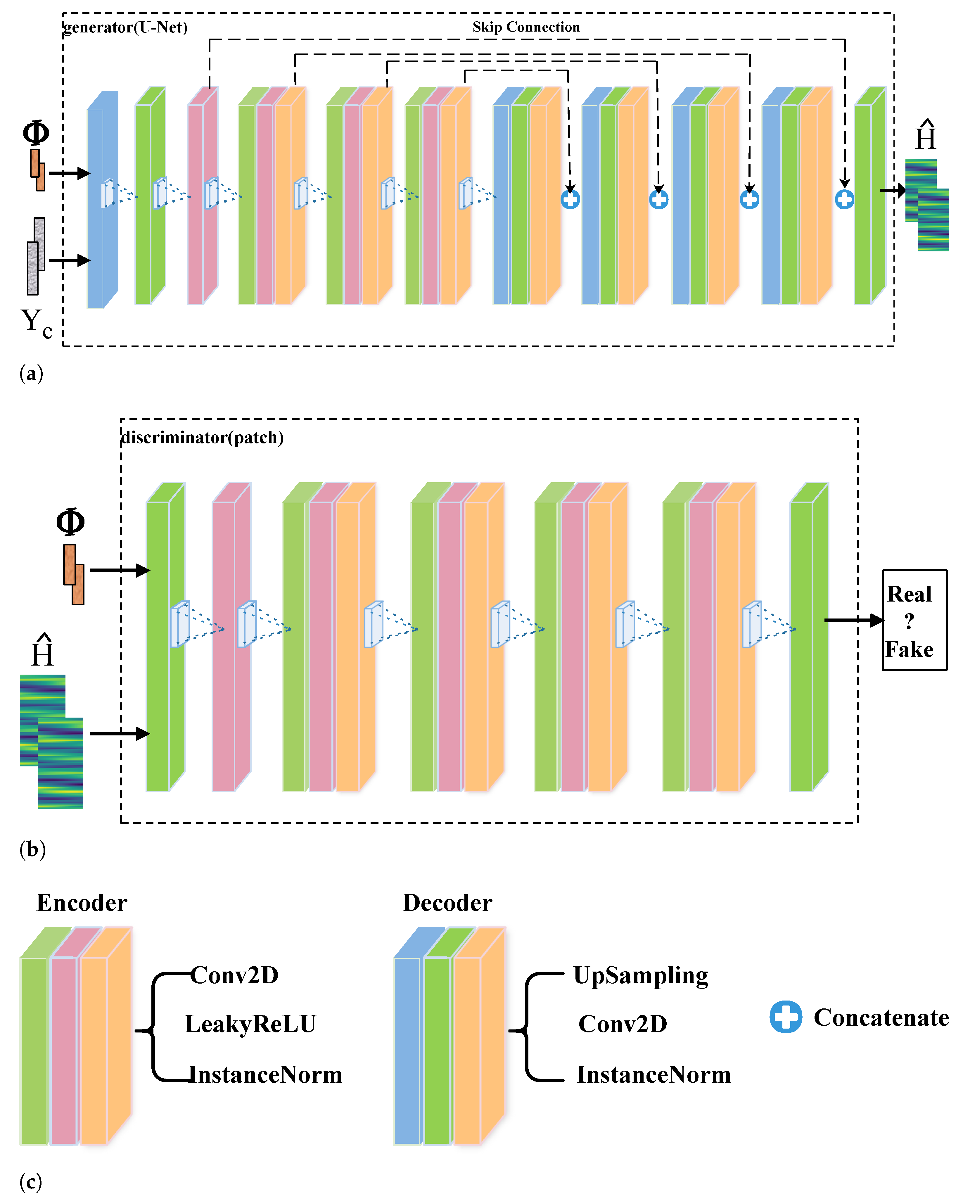
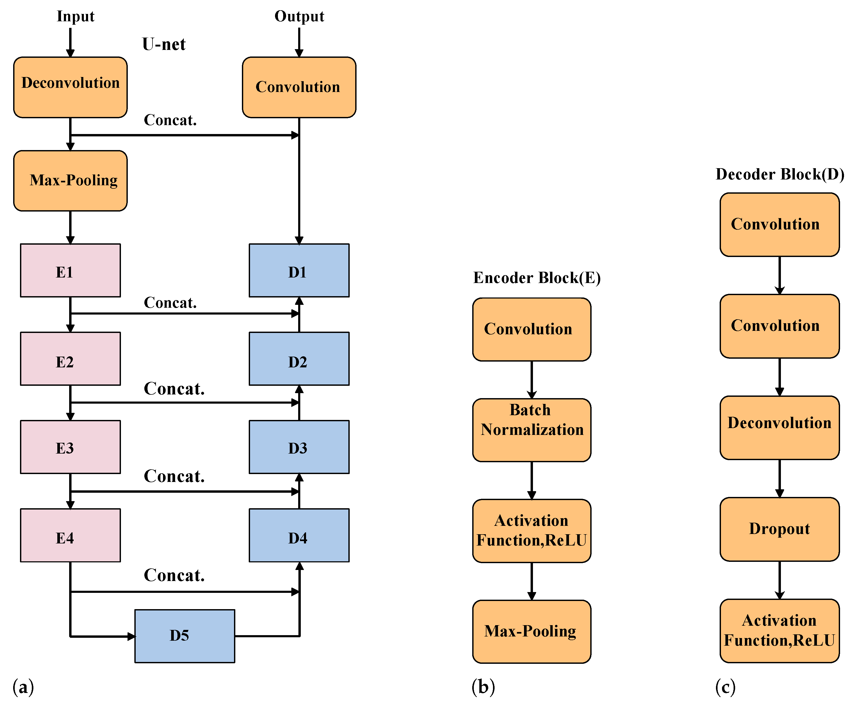
In N2N-cGAN algorithm, both the denoising network and the generative network use the U-Net framework. U-Net is a CNN designed for semantic image segmentation. The structure of U-Net can be divided into downsampling and upsampling. Both of them use the encoder and decoder as well as the jump connection topology, which allows for more precise segmentation on fewer training images. U-Net is symmetrical. The expansion path on the right side of the network is symmetrical with the contraction path on the left to restore the size of the picture, while the contraction path on the left is used to capture context information. The output feature map of the encoder corresponding layer is copied, cut, and deconvoluted for feature fusion through jump connection, The output feature mapping of the corresponding layer of the encoder is copied, cut, and deconvoluted, and the feature fusion is carried out through the jump connection, and then the upsampling operation is carried out. During the upsampling process, U-Net employs many feature channels, which can improve the quality of the output and the accuracy of the segmentation.

Algorithm 1 N2N-cGAN-Based Channel Estimation

Require:$\Phi$,H. Ensure:${\stackrel{\Lambda }{Y}}_{\mathrm{c}}$.   1: for number of training iterations do   2:    Construct sample of $Y_c$ (16)   3:    Construct two samples of Y and $Y^{\prime }$ (17)   4:    Obtain $D_{n\theta }\left(Y\right)$ with Y.   5:    Update the $D_{n\theta }\left(\cdot \right)$ by the loss function (20).   6: end for   7: Extract the trained $D_{n\theta }\left(\cdot \right)$.   8: Get the clean pilot: $\stackrel{\Lambda }{Y_{\mathrm{c}}}=D_{n\theta }\left(Y^{*}\right)$. Require: ${\stackrel{\Lambda }{Y}}_{\mathrm{c}}$. Ensure: $\stackrel{\Lambda }{H}$.   9: for number of training iterations do   10:    Sample minibatch of data ${\stackrel{\Lambda }{Y}}_{\mathrm{c}}$ and data H.   11:    Train $G_{\Phi }$ and $D_{\omega }$ alternately by (21) and (22) with ${\stackrel{\Lambda }{Y}}_{\mathrm{c}}$ and H.   12: end for   13: Obtain the trained generator network $G_{\Phi }$.   14: Get the channel estimation:$H=G_{\Phi }\left(Y_c^{*}\right)$.

Figure 4a shows the architecture of the denoising network. The input image resolution is $M\times N_p$. We first use a deconvolution to change the shape to adapt to the convolution operation. The next encoder consists of four submodules, each of which contains a convolution layer, a batch normalization layer, and each submodule has a downsampling layer realized by max-pooling as shown in Figure 4b. After this processing, the image size becomes $2\times 1\times 512$. The information flow enters the decoder on the right side. The decoder also includes five submodules. Each submodule is composed of two convolution layers and a dropout layer, and each submodule has an upper sampling layer realized by deconvolution as shown in Figure 4c. The resolution is improved by upsampling operation. Finally, the output image has the same resolution as the input image in the convolution process. The jump connection connects the upsampling result with the output of the submodule of the encoder, whose connection part has the same resolution, and takes it as the input of the next submodule in the decoder.

The discriminator network uses CNN. As shown in Figure 5b. Instead of acting as a discriminator to discriminate true from false by mapping the input to a single scalar output, the input is mapped to the receptive field via a patch discriminator [41], with each element indicating whether the input block is true or not. The front-end part of the discriminator consists of a convolutional layer, a LeakyReLU activation layer, and four encoder blocks. Each convolutional layer consists of 512 4 × 4 sized filters. We use the full connected layer in the last layer instead of the convolutional layer to obtain the receptive field. The final output of the discriminator is then produced by averaging all the answers from the receptive field.

4. Numerical Results and Analysis

In this section, we use simulations to evaluate the performance of the N2N-cGAN algorithm and compare it with other approaches. Reference [31] has demonstrated through experiments that cGAN outperforms U-Net and CNN in terms of accuracy for channel estimation directly from noisy pilots. The work also considers the case where the length of the pilot sequence is smaller than the number of transmitting antennae, but the scenario considered in this paper is more complex, making the comparison results more informative. This paper mainly examines the performance of the N2N-cGAN and cGAN estimation methods compared to traditional channel-estimation algorithms LS and MMSE from three aspects. First, simulation parameters are set, and the standard for channel-estimation performance is established. Then we compare the performance of the proposed algorithms from different SNRs and different numbers of antennae deployed at the BS. Finally, we also compare the computational costs of different algorithms.

4.1. Simulation Dataset

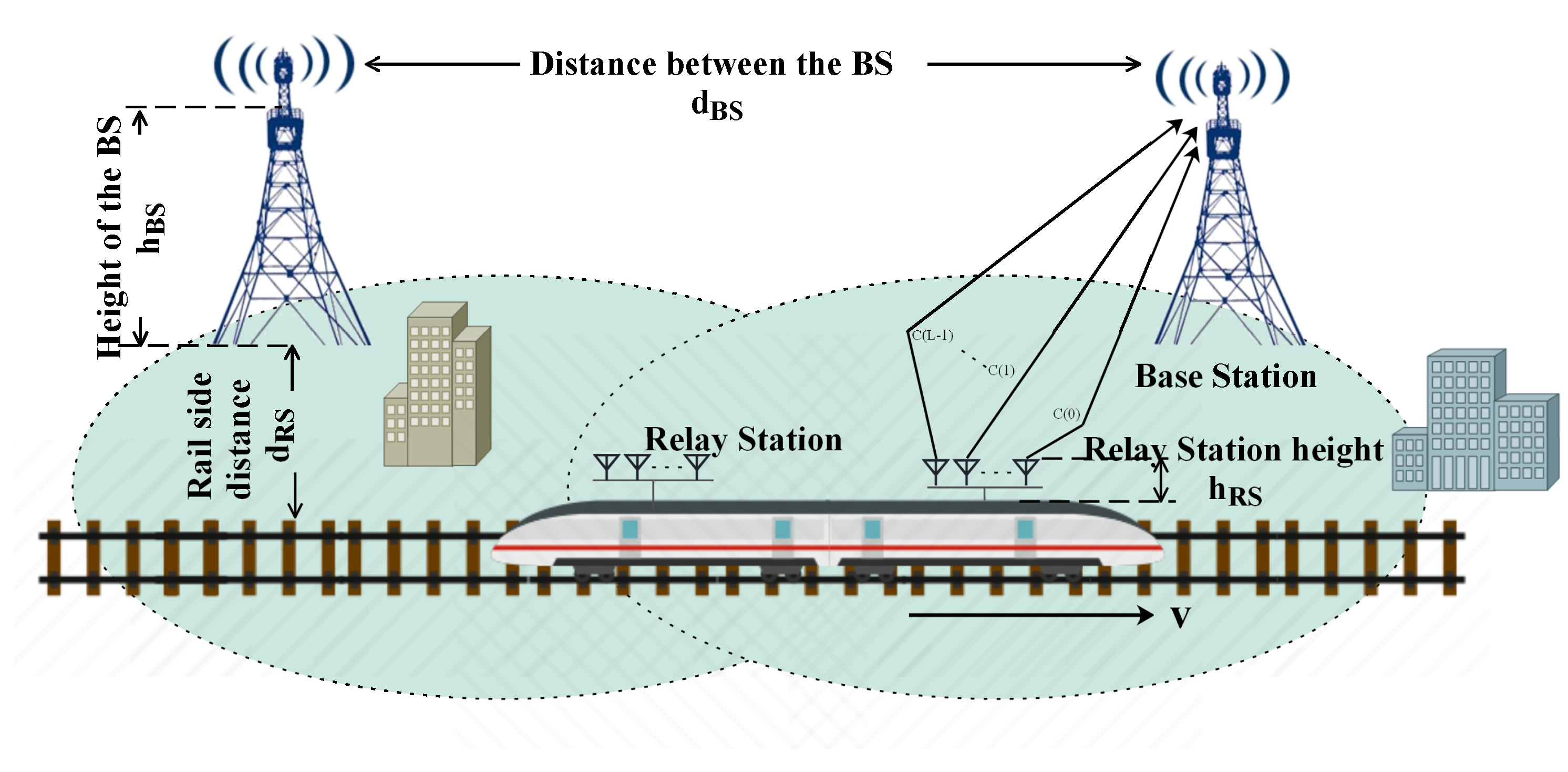
In our study, simulation data is produced by using the WINNER II D2a channel model. It is a scenario model for mobile devices, its network coverage, antenna configuration, and moving speed are all suitable for the HSR scenario described in this paper. Its channel parameters ( RMS, path loss, etc.) are derived from the calculations in Section 2. Therefore, this channel model will be used in this paper to complete the simulation under the high-speed rail channel. The scene layout measured by WINNER II D2a includes the following. The RS is atop the moving train, whereas the BS is 50 m from the rail, that is $d_{RS}=50$ m. The link between the BS and the moving RS is basically considered to be LOS. The height of the BS is $h_{BS}=30$ m. The height of the RS on the top of the train is $h_{RS}=2.5$ m. The train speed is $v=360$ km/h.

Table 1. Simulation parameter.

Parameter	Symbol	Value
Number of subcarriers	N	64
Carrier frequency		$3.5$ GHz
Number of multipaths	L	5
Modulation		QPSK
Channel model		WINNER II D2a
The speed of the train	V	360 km/h
Number of transmit antennae	$N_T$	$64,$$128,$$192,$ 256
Number of receive antennae	$N_R$	32
Pilot length	$N_p$	$4,$$8,$ 16

displays the other specific simulation parameters.

According to these parameters, the channel vector between each user and the antenna array are generated. The user sends the derivative symbols as $\left\{\frac{1}{N_p}{e}^{j\frac{k\pi }{2N_p}},k=0,1,\dots ,N_P\right\}$, These symbols are freely combined to form a sequence of U derivatives, which generate the derivative matrix $\Phi$ of U × $N_p$.

Through the channel model, the 10,000 real channel dataset is obtained. The z-score standardized method was used to process the dataset. The mean value of the processed dataset is 0 and the standard deviation is 1, which is more suitable for model training. Then, to produce clean pilots, we combine the normalized actual channel data with the Formula (16). The noise-containing pilots are obtained by adding independent Gaussian white noise under a given SNR. Consequently, a clear pilot dataset and a noisy pilot dataset are thus obtained. Finally, we reduce the three datasets’ complicated data into two-channel picture data, and use the holdout method in the divided dataset. It is divided into a training set and a test set according to the ratio of 4:1.

At the simulation stage, the Gaussian white noise under the SNR of $-10$ dB to 10 dB is superposed by the clean signal to generate multiple noise-containing signals. Since the noisy signals all come from the same clean signal, the initial training data of the denoising model are freely combined by them. In the second stage, the cGAN takes the clean signal as input directly, with the actual channel data serving as the training data for the generator model. The two training stages can be conducted concurrently in this manner. The denoiser, generator, and discriminator are employed with the Adam optimizer with learning rates of $1\times {10}^{-3}$, $2\times {10}^{-4}$, and $2\times {10}^{-4}$, respectively, to train the proposed N2N-cGAN model. As a comparison of the end-to-end cGAN method, we use noisy pilot data as the generator input, while real channel data serves as the generator learning object.

4.2. Evaluation Criteria

In the simulation, we quantify the variance between the estimated channel $\stackrel{\wedge }{H}$ and the real channel H by using the normalized mean square error (NMSE) as the evaluation standard. This is expressed as

$$NMSE=10{log}_{10}\left\{\mathbb{E}\left[\frac{{∥H-\stackrel{\wedge }{H}∥}^2}{{∥H∥}^2}\right]\right\},$$

(25)

where the matrix norm computation is shown by the symbol $∥\cdot ∥$ and $\mathbb{E}$ obtains values of expectation. To facilitate the observation of simulation results, we calculate $10{log}_{10}\left\{\cdot \right\}$ to convert NMSE into dB form.

4.3. Performance Evaluation

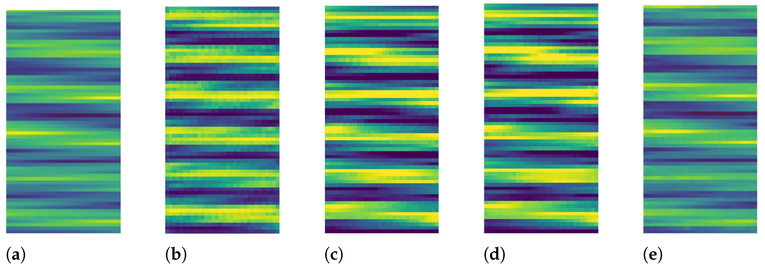
First, Figure 6 shows the display of channel estimate results by using various methodologies. We visualize the estimated and real channels as graphics in pseudocolor images.

The simulated data was generated with an SNR of 0 dB and a pilot sequence length of 8. The resulting estimated channel matrix $\stackrel{\wedge }{H},$ and the real components of the actual channel matrix H are presented as pseudocolor images. The color values correspond to the data values in the channel matrix. As we can see from Figure 6a–e, the visual images obtained by the LS estimation algorithm, MMSE estimation algorithm, and cGAN estimation algorithm are very different from that of the real channel. However, the N2N-cGAN-generated channel picture closely resembles the real channel. This indicates that the N2N-cGAN method generates channel details well. That is, results from the N2N-cGAN channel estimate can be more realistic.

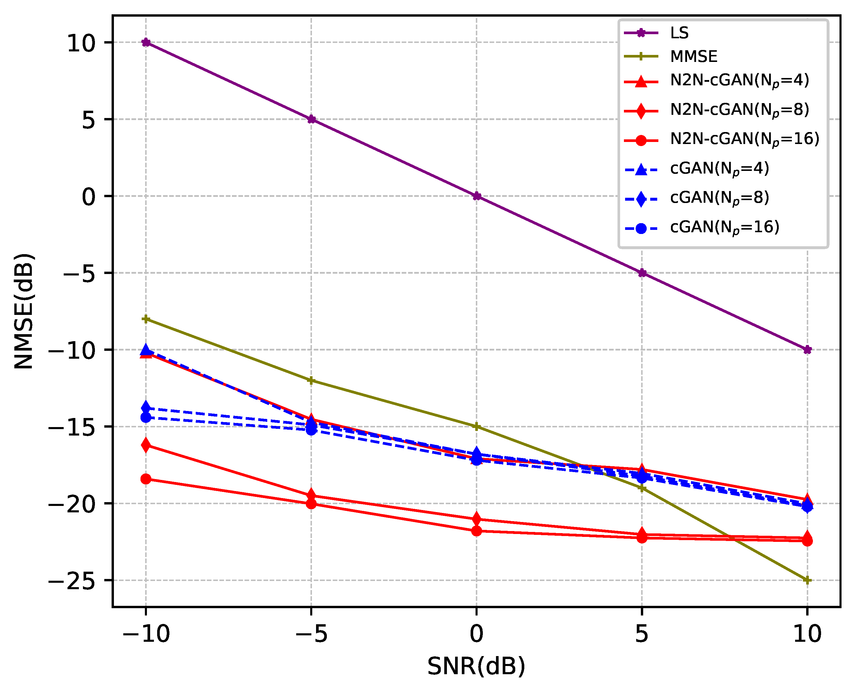
Figure 7 illustrates the comparison of NMSE performance between N2N-cGAN and cGAN algorithms, as well as conventional LS and MMSE algorithms, under different SNRs.

It shows the MMSE values obtained by the four channel-estimation methods in the process of SNR changing from $-10$ dB to 10 dB. N2N-cGAN and cGAN use pilot sequences to estimate channels with lengths of 4, 8, and 16 respectively. The comparative analysis of estimated errors between the N2N-cGAN and cGAN demonstrates that, irrespective of the variation in SNR and pilot sequence length, the N2N-cGAN outperformed the cGAN in terms of estimated error. Notably, the estimated error of N2N-cGAN is much smaller than that of cGAN when the pilot length is 8 or 16 and the SNR is low. Additionally, Figure 7 shows that when the duration of the pilot sequence reduces, the estimation errors of both techniques increase, and the change in performance of N2N-cGAN is relatively more obvious, and the performance of N2N-cGAN at the pilot sequence of the length of 4 is comparable to that of cGAN at a pilot sequence of length 16. N2N-cGAN is overall better than cGAN. It is mainly because the first stage denoising network in N2N-cGAN removes the noise from the noisy pilot as much as possible, which makes the second stage channel estimation approximate for a noise-free estimation. In contrast, cGAN directly uses noisy pilots to estimate the channel, which makes cGAN learn the change of noise. However, the noise is independent and unpredictable, so the estimation error of cGAN will be greater than that of N2N-cGAN, which is more obvious in the case of low SNR. Lastly, Figure 7 demonstrates that the classic LS approach performs the worst. In the event of high SNR, the performance of the MMSE method can outperform N2N-cGAN, but it is not even superior to the cGAN estimation method at low SNR.

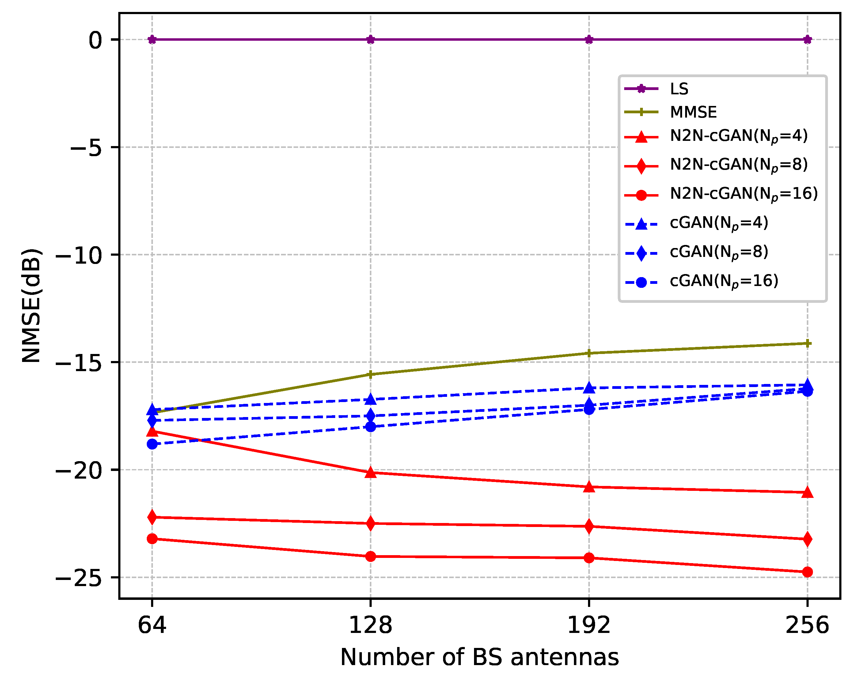
Next, We analyze the NMSE performance of LS, MMSE, cGAN, and N2N-cGAN in different scenarios where the number of antennae deployed in the BS varies. The SNR is 0 dB in this simulation. The corresponding simulation results are presented in Figure 8. It demonstrates that the N2N-cGAN estimation approach exhibits superior performance compared to the cGAN approach, as the estimation error decreases with the increase of the number of antennae. The size of the channel matrix will expand as the number of BS antennae rises. The use of cGAN for estimation results in a complex estimated target, which increases the learning difficulty and consequently leads to reduced performance. For N2N-cGAN, the performance of the second stage is almost not affected due to the noise-free estimation. The denoising of the first stage learns better denoising methods because of the introduction of more noise information, so the performance of N2N-cGAN improves with the increase of antenna numbers. Figure 8 illustrates that the performance of the MMSE approach deteriorates as the number of antennae increases, while the estimation error of the conventional LS method remains relatively constant. As the pilot sequence length increases from 4 to 8, the performance improvement of N2N-cGAN is more significant, which can be shown from the simulation. However, when the length is further increased from 8 to 16, the performance gain of N2N-cGAN is less significant.

4.4. Complexity Analysis

Table 2. Computational complexity.

Algorithms	Number of Multiplication Operations	Complexity
LS	$N_r{N}_{t}N$	$O\left(N\right)$
MMSE	$N_t{N}_r(3N^3+N^2)$	$O\left(N^3\right)$
cGAN	$N_t{N}_r\left(3N^2\right)$	$O\left(N^2\right)$
N2N-cGAN	$N_t{N}_r(3N^2+N)$	$O\left(N^2\right)$

presents the results. The computational complexity of the four channel-estimation algorithms, LS, MMSE, cGAN, and N2N-cGAN, are measured in terms of the number of complex multiplications. In the table, $N_r$ and $N_t$ represent the number of receiving and transmitting antennae respectively, and N represents the number of subcarriers.

Among the channel-estimation algorithms, the LS algorithm exhibits the lowest computational complexity. The MMSE has the highest computational complexity due to matrix inversion. The N2N-cGAN algorithm exhibits low computational complexity, as it only involves matrix multiplication and addition, and does not require matrix inversion operations. Online complexity is less difficult than traditional MMSE complexity. Additionally, because the neural network may be constructed in parallel, the approach can shorten the algorithm’s execution time. The complexity of the online implementation phase of the algorithm is low, because the trained model can be used immediately for channel estimation without large computational overhead.

5. Conclusions

This paper proposes a channel-estimation scheme based on N2N-cGAN for HSR wireless communication system. Specifically, we propose a two-stage channel-estimation algorithm based on N2N-cGAN. The pilot matrix is regarded as an image. The noise-containing pilot image is denoised by the N2N denoising algorithm, which makes the model suitable for scenarios with strong channel noise. Then the important features of these images are learned by using the cGAN to realize the channel-estimation process. The simulation results based on actual deployment scenarios show that the developed solution can effectively improve the channel-estimation accuracy in high-speed mobile environments, and the proposed solution can obtain lower estimation errors than other methods. In addition, with the increase of pilot sequence length, the performance of N2N-cGAN improves better.

Although our work can effectively improve the accuracy of channel estimation, it relies heavily on the quality and quantity of training data. Therefore, the performance of the proposed method may be affected by the variability of the wireless communication environment and the availability of training data. Future research can focus on developing more effective training strategies or selecting appropriate training data, adjusting hyperparameters, and optimizing network structures to improve model performance and generalization.