The Online Frequency Security Assessment of a Power System Considering the Time-Varying Characteristics of Renewable Energy Inertia

Abstract

The continuous increase in the penetration rate of renewable energy has led to a decrease in the system’s frequency response capability, which presents great challenges to the safety and stability of the power system. In order to ensure the safe operation of the power system, online frequency safety assessment has become necessary. However, the time-varying characteristics of the virtual inertia H_NE of renewable energy stations make it more difficult to accurately predict the lowest point of the system frequency after a disturbance. Based on the general average system frequency (G-ASF) model, this paper proposes a G-ASF-H model that considers the time-varying characteristics of the virtual inertia of renewable energy stations, accurately predicts the lowest frequency point after a system disturbance, and realizes the online frequency safety assessment of the system. Firstly, a unified virtual synchronous generator model is established to identify the virtual inertia time constant of the renewable energy station in real time; then, under the pre-defined frequency safety verification event, the maximum deviation of the system frequency is periodically calculated and judged based on the G model to realize the online frequency safety assessment. The example analysis on the IEEE 10-machine 39-node system shows that the model has a high calculation speed and accuracy under different disturbances or daily load level scenarios and can be used for the online security assessment of new power systems with time-varying virtual inertia characteristics.

1. Introduction

A low-carbon and clean energy structure has become the development direction of future energy patterns. In this context, the renewable energy industry, represented by wind power and photovoltaics, has developed rapidly [1,2,3,4]. For renewable energy systems, such as wind energy and photovoltaic (PV) systems, the maximum power point tracking (mppt) operation mode decouples the rotor kinetic energy from the grid frequency and cannot provide rotational inertia support for frequency changes when the grid frequency is disturbed [5]. The increased intermittent renewable energy penetration is accompanied by the application of a large number of power electronic devices, making the model order high and the time domain simulation modeling work more cumbersome, bringing new technical challenges to the system frequency stability analysis [6]. Large-scale renewable energy grid connections will result in strong random disturbances to the power grid [7,8,9,10], and system frequency instability is likely to occur due to the inertial decline of conventional units and the lack of auxiliary frequency support [11,12,13]. The contradiction between the penetration rate and the safe and stable operation of the power grid has become increasingly prominent.

Power system frequency stability is usually verified by simulation, but frequency stability under simulation verification events is mainly performed offline, and requires a large amount of calculation. Monitoring, as the core function of the energy management system (EMS), is usually performed by conducting an online safety assessment every 5 to 15 min, which mainly takes into consideration static safety issues, such as the voltage and current exceeding the limits. As frequency stability problems worsen, it becomes necessary and valuable to supplement the frequency stability in the online evaluation process.

To improve the frequency stability of the power grid, it is necessary to encourage renewable energy units to participate in frequency support [14,15,16,17]. At the same time, to solve the dynamic frequency security problem of the power grid caused by the gradual increase in the penetration rate of renewable energy, virtual synchronous control technology has become more widely used in the actual grid. For example, the virtual synchronous control technology used in photovoltaic systems draws on the electromechanical characteristics of the conventional power system, such that the inverter is equivalent to the synchronous machine in terms of the internal and external characteristics, thereby providing inertial support for the system. Wind power systems also achieve significant improvements in the equivalent inertia of the system by using its moment of inertia and the virtual synchronous control of the converter. Previous studies have found that the frequency change rate and the maximum frequency deviation of the power system are affected by the equivalent inertial time constant of the system after a power imbalance occurs, and the most concerning feature of the frequency safety assessment is the lowest point of the frequency. Therefore, accurate identification of the renewable energy equivalent virtual inertial time constant (H_NE) is beneficial for measuring the inertia support level of renewable energy to the power grid, and to lay a solid foundation for the calculation of the maximum frequency deviation of the new power system under large disturbances.

For the calculation of the maximum frequency deviation of the new power system under large disturbances, simulation software such as PSCAD or PSASP can give a complete frequency curve within a high precision range, but its efficiency with respect to time is not sufficient to be able to perform online safety assessments in a large power grid. It is worth noting that the online frequency safety assessment does not require a complete and accurate frequency curve, but rather some specific points; therefore, an equivalent model can be applied to achieve a high calculation speed.

Several equivalent models for calculating the maximum frequency deviation have been proposed in the literature that are able to greatly reduce the volume of calculations and increase the calculation speed. The average system frequency (ASF) model considers different types of speed control systems and is widely used in primary frequency response (PFR). However, when the ASF model is applied to a large power grid, there are problems such as high-order, difficult calculations, and high cost. On the basis of the ASF model, the research in [18,19] adopted a low-order polynomial speed control system model and performed open-loop processing to realize the calculation of the lowest point of the frequency, but they did not consider renewable energy stations. Ref. [20] proposed a low-order general model of a generator speed control system that took the frequency response characteristics into full consideration, combined with the general frequency response model of renewable energy stations, and established a general average system frequency (G-ASF) model for renewable energy access to the grid. However, the virtual inertia of the renewable energy station in the new power system will have time-varying characteristics, meaning that the maximum frequency deviation of the G-ASF model will be calculated inaccurately in scenarios with time-varying virtual inertia. Therefore, it is necessary to identify the renewable energy station H_NE in this scenario in real time.

Regarding H_NE identification, ref. [21] used the dynamic mode decomposition (DMD) method to identify the inertia of synchronous generators based on the swing equation, but it was not further applied to renewable energy stations. Ref. [22] proposed a damping and moment of inertia test method based on the power angle transfer function by analyzing the power angle characteristics of the photovoltaic virtual synchronous generator. However, this method was only suitable for small power disturbances. In the case of large disturbances, the error of the model linearization was relatively large, and there were certain limitations. Ref. [23] defined the concept of the system average frequency and evaluated the equivalent inertia of the wind farm by collecting the angular frequency of the doubly fed wind turbine. Ref. [24] proposed a renewable energy station virtual inertia estimation method based on dynamic mode decomposition. A renewable energy station frequency characteristic estimation model was constructed on the basis of the dynamic mode decomposition algorithm.

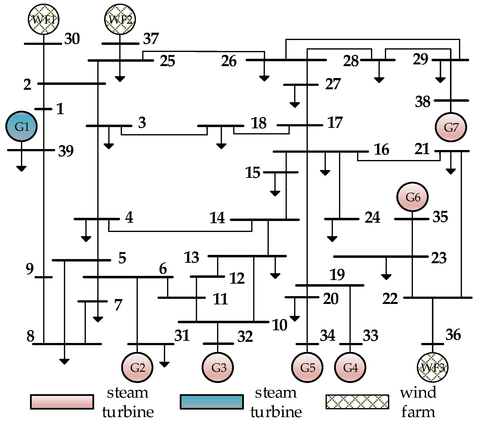
Considering that the renewable energy field station provides inertia support for the system, and the virtual inertia has time-varying characteristics, this paper first establishes a unified virtual synchronous generator model (U-VSG) and uses online monitoring data and the genetic algorithm to realize the real-time identification of the virtual inertia time constant of the renewable energy station; then, combined with the general average system frequency (G-ASF) model, an online frequency safety assessment G-ASF-H model considering the time-varying characteristics of the virtual inertia of renewable energy stations is proposed. Finally, a simulation example consisting of 10 machines and 39 nodes was established in PSCAD/EMTDC, on the basis of which it was verified that the proposed model has a high calculation speed and accuracy under different disturbances or daily load level scenarios, and can be used for the online frequency safety assessment of new power systems with time-varying virtual inertia characteristics.

This paper is organized as follows. In Section 2, we first briefly introduce the G-ASF model [20]. Based on the G-ASF model, the G-ASF model for frequency nadir prediction considering the time-varying characteristics of virtual inertia H_NE is proposed. In Section 3, we identify the virtual inertia of the renewable energy station and predict the lowest frequency point after system disturbance. The application of the G-ASF model in online frequency security assessment is described. The performance of the G-ASF model in online frequency security assessment is validated using a single-generator system, a New England 39-bus system, and a regional power system in Section 4. Section 5 presents the conclusions.

2. G-ASF-H Model for Real-Time Identification of Renewable Energy Station Inertia

2.1. G-ASF Model Architecture

The virtual inertial response is used to introduce the response into the frequency differential in the power control of the renewable energy station, so that renewable energy stations will be able to simulate the inertial response of synchronous generator rotors. The additional power reference value P_Href generated by the virtual inertial response of the renewable energy station is

$$\Delta P_{\mathrm{Href}}=\frac{2H_{NE}}{f_N}\frac{df}{dt}.$$

(1)

In the formula, H_NE is the virtual inertial time constant of the renewable energy station rotor (H_NE = 0 means that the renewable energy station does not provide a virtual inertial response), and f_N is the rated frequency.

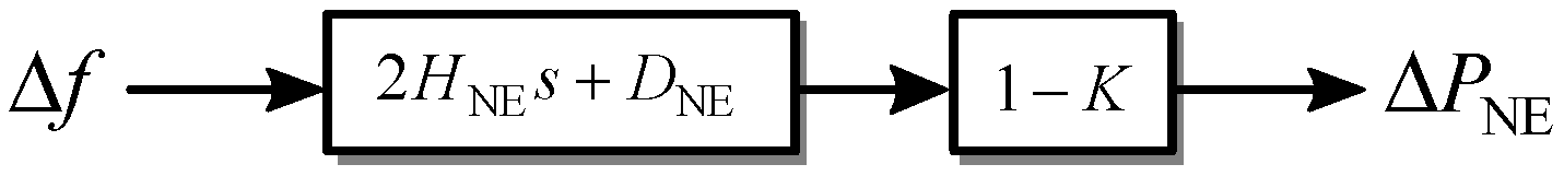
The general frequency response model of the renewable energy station is shown in Figure 1. Its input is the variation in grid frequency, and its output is the variation in frequency response power.

In the figure, D_NE is the droop coefficient (D_NE = 0 means that the renewable energy station does not provide a frequency damping response), that is, the frequency damping provided by the renewable energy station; 1 − K is the conversion coefficient of renewable energy per unit value.

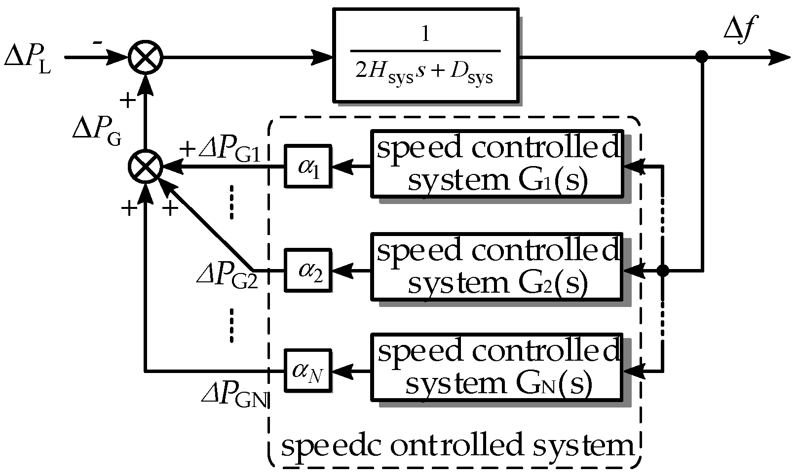
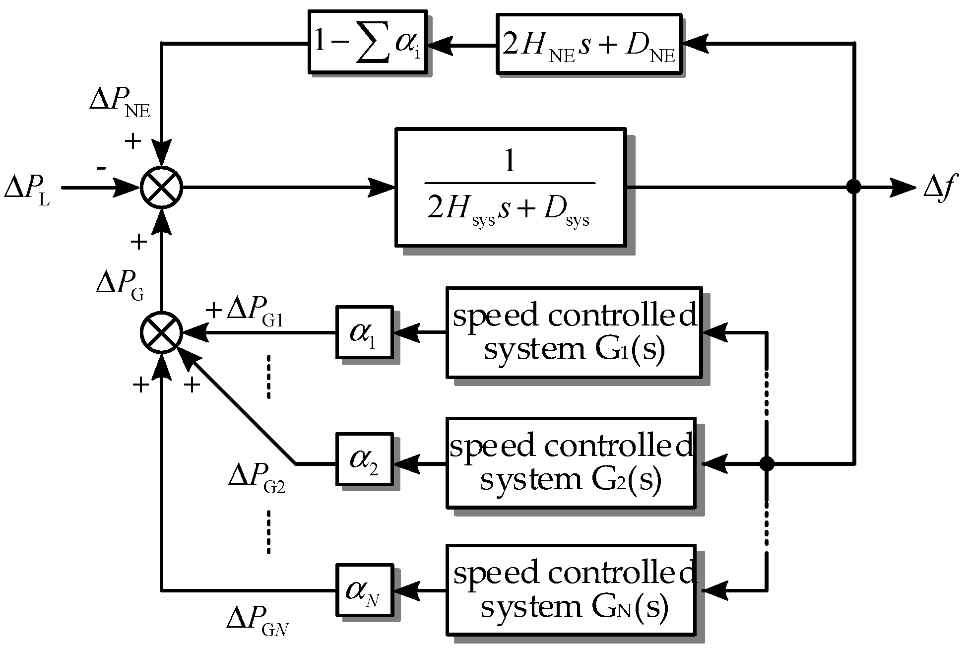
It is difficult to obtain an accurate and simplified mathematical model of the speed control system using the traditional ASF model. Ref. [20] proposed a low-order general model of the generator speed control system that fully considered the frequency response characteristics by establishing a general average system frequency (G-ASF) model. The G-ASF model is shown in Figure 2.

In the figure, α_i is the per unit value conversion coefficient, H_sys is the equivalent inertia time constant of the system, D_sys is the equivalent damping coefficient of the system, Δf is the system frequency deviation, ΔP_L is the unbalanced power that appears after the system is disturbed, ΔP_G is the output mechanical power change in the generator speed control system after the frequency fluctuation, and G_i(s) is the transfer function of the i-th speed control system. According to Figure 2,

$$H_{sys}=({\displaystyle \sum _{i=1}^{N_G}{H}_i\cdot S_i})/{\displaystyle \sum _{i=1}^{N_G}{S}_i},$$

(2)

$$D_{sys}=({\displaystyle \sum _{i=1}^{N_G}{D}_i\cdot S_i})/{\displaystyle \sum _{i=1}^{N_G}{S}_i},$$

(3)

$$\Delta f=({\displaystyle \sum _{i=1}^{N_G}{H}_i\cdot \Delta f_i})/H_{sys}.$$

(4)

In these formulas, S_i, H_i, D_i, and Δf_i are the rated capacity, inertia time constant, damping coefficient, and frequency of generator i, respectively; N_G is the number of generators participating in the frequency response in the grid.

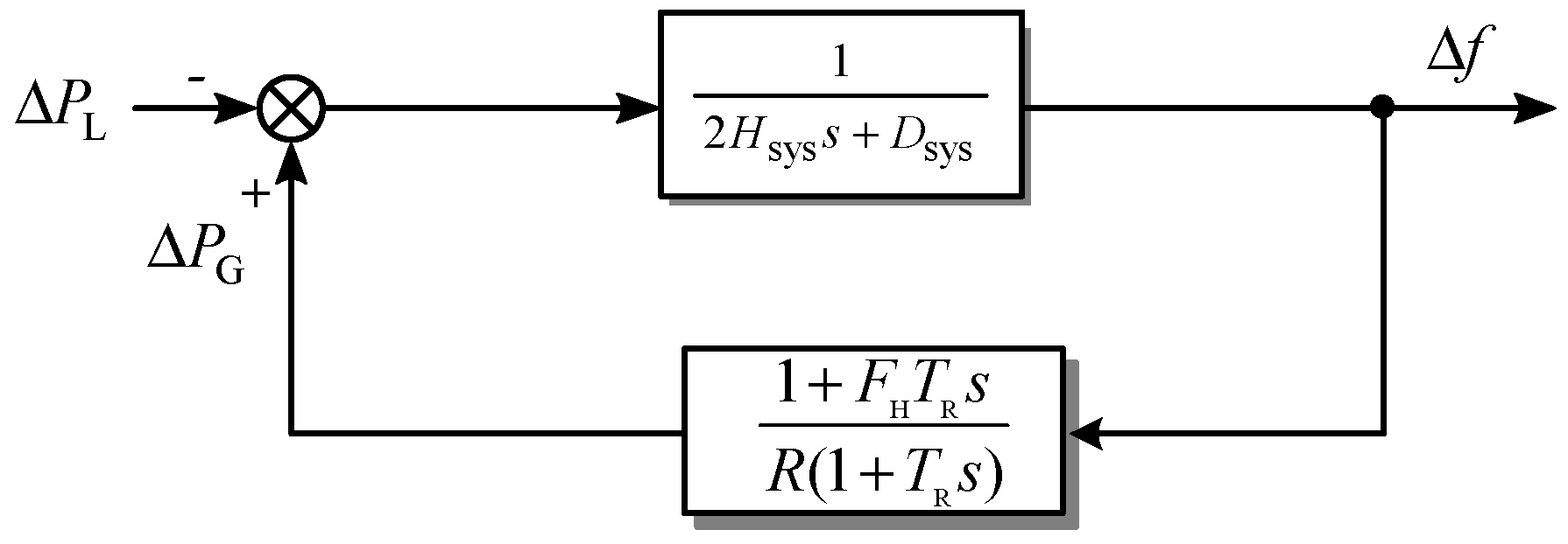
The classical system frequency response (SFR) model is shown in Figure 3. Based on the ASF model, it is assumed that the frequency of the entire power system is uniform, and a reheating link speed control system is equivalent to the frequency control of all units; therefore, the system is transformed into a single-unit model. In the figure, F_H is the working ratio of the equivalent high-pressure cylinder; T_R is the equivalent reheat time constant; R is the adjustment coefficient.

The SFR model is a second-order model, and the analytical expression of the frequency dynamic response after power system disturbance occurs can be directly calculated through the model. The structure of the SFR model is simple, the volume of calculation is small, and the minimum frequency can be quickly predicted. However, this model requires that all generator sets must be of the reheat steam engine type, and all governor prime mover models must be the same; if other types exist, then this model does not apply. Therefore, the SFR model has poor generalization and accuracy.

2.2. Unified VSG Model of Renewable Energy Stations

The G-ASF model proposed in [20] considers the supporting effect of the renewable energy station on the system frequency, but the H_NE of the general frequency response model of the renewable energy station is a known quantity. Ignoring the fact that the H_NE is unknown under the special frequency control method of the renewable energy field station means that it is impossible to quickly and accurately predict the system frequency deviation after being disturbed.

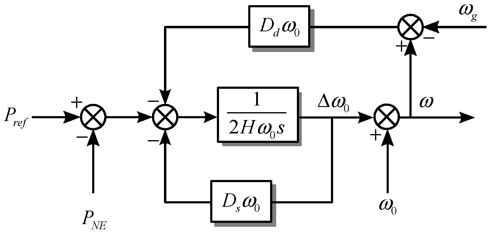
Based on the idea that the equivalent value of renewable energy stations with inertia characteristics is VSG [25], a unified VSG model is obtained, as shown in Figure 4. The real-time prediction of renewable energy station H_NE is realized through data measurement and the genetic algorithm, which lays the foundation for predicting the minimum frequency of renewable energy access to the grid.

In the figure, P_NE is the output power generated by the frequency response of the renewable energy station, ω₀ is the rated angular frequency, ω_g is the grid angular frequency, D_d is the dynamic damping coefficient, and D_s is the steady-state damping coefficient.

2.3. G-ASF-H Model Considering the Inertia of Renewable Energy Stations

The unified VSG model including renewable energy stations was added to the G-ASF model, and the G-ASF-H model for real-time prediction of renewable energy station H_NE was obtained, as shown in Figure 5.

Based on the original G-ASF model, the G-ASF-H model considers the impact of the changes in the control strategy of renewable energy stations on the H_NE, realizes real-time updates of the H_NE of renewable energy stations, and avoids the excessive prediction error of the minimum frequency point caused by the change in the H_NE of the renewable energy station. The G-ASF-H model provides a theoretical basis for the prediction of the lowest point of the system frequency in the case of the unknown renewable energy station H_NE. It should be emphasized that this model still has the original advantages of the G-ASF model. When the system structure changes greatly, such as when the generator is replaced by a renewable energy station, the corresponding speed control system model only needs to be removed [20]. At the same time, through the real-time identification of the renewable energy station H_NE, it is enough to modify the unified VSG model parameters of the renewable energy station. When it is necessary to analyze the lowest point of the frequency under different unit combinations, it is only necessary to combine the previously established speed control system models without remodeling the overall power grid, which greatly improves the flexibility and practicability of the model.

3. Online Frequency Security Assessment Based on the G-ASF-H Model

3.1. H_NE Identification Method for Renewable Energy Stations

To evaluate the inertia support of the renewable energy station to the power grid, it is necessary to establish a unified model of VSG through the H_NE identification method when the control strategy or parameters adopted inside the renewable energy station are unknown. According to the different simulation methods of the VSG, Equations (5) and (6) can be used to characterize the governor and rotor motion equation:

$$\Delta P=K_{\omega }({\omega }_0-\omega )+K_{\omega }(\omega -{\omega }_g),$$

(5)

$$P_{\mathrm{ref}}+\Delta P-P=2H_{\mathrm{NE}}{\omega }_0\Delta \omega s+D_1{\omega }_0(\omega -{\omega }_g)+D_2{\omega }_0(\omega -{\omega }_0).$$

(6)

In the formula, ΔP is the amount of power change, K_ω is the proportional coefficient of the governor, P_ref is the power reference value of VSG, P is the output active power of VSG, D₁ and D₂ are the damping coefficients, and s is the complex frequency.

When the internal control strategy of the renewable energy station is unknown, the external characteristics of the VSG in different forms can be simulated by adjusting the values of K_ω, D₁, and D₂ in Formulas (5) and (6); therefore, the control strategy corresponding to Equations (5) and (6) is selected as the control strategy of the unified external characteristic model for the inertia identification of renewable energy stations.

Substituting Formula (5) into Formula (6), we obtain

$$\left\{\begin{array}{l}{P}_{\mathrm{ref}}-P=J{\omega }_0\Delta \omega s+D_{\mathrm{d}}{\omega }_0(\omega -{\omega }_{\mathrm{g}})+D_{\mathrm{s}}{\omega }_0({\omega }_0-\omega )\\ D_{\mathrm{d}}=D_1-\frac{K_{\omega }}{{\omega }_0}\\ D_{\mathrm{s}}=D_2+\frac{K_{\omega }}{{\omega }_0}\end{array}\right..$$

(7)

In the formula, J is the moment of inertia.

According to Formula (7), the unified VSG model can be obtained as shown in Figure 4. To simplify the analysis, we let P_ref = 0, and we apply the small signal perturbation to Formula (7):

$$\Delta P=(-2H_{\mathrm{NE}}{\omega }_0\Delta \omega s-D_d{\omega }_0-D_s{\omega }_0)\Delta \omega +D_d\omega \Delta {\omega }_g.$$

(8)

We define k_g as the gain from the phase angle difference between the VSG output voltage and the grid voltage to the VSG output active power P:

$$\Delta P=(\Delta \omega -\Delta {\omega }_{\mathrm{g}})\frac{1}{s}{k}_{\mathrm{g}}.$$

(9)

Simultaneously, Formulas (8) and (9) become

$$\begin{array}{ll}G(s)& =\frac{\Delta P}{-\Delta {\omega }_{\mathrm{g}}}=\frac{k_{\mathrm{g}}(2H_{\mathrm{NE}}{\omega }_{0}s+(D_{\mathrm{d}}+D_{\mathrm{s}}){\omega }_0-D_{\mathrm{d}}{\omega }_0)}{2H_{\mathrm{NE}}{\omega }_0{s}^2+(D_{\mathrm{d}}+D_{\mathrm{s}}){\omega }_{0}s+S_E}\\ & =\frac{b_{1}s+b_0}{a_2{s}^2+a_{1}s+a_0}\end{array}$$

(10)

$$\left\{\begin{array}{l}{b}_1=k_g\\ b_0=k_g((D_d+D_s){\omega }_0-D_d{\omega }_0)\\ a_2=1\\ a_1=(D_d+D_s)/(2H_{\mathrm{NE}})\\ a_0=k_g/(2H_{\mathrm{NE}}{\omega }_0)\end{array}\right..$$

(11)

In Formula (10), S_E is the gain from the phase angle difference between the VSG output voltage and the grid voltage to VSG output power P.

The genetic algorithm refers to a metaheuristic algorithm influenced by genetics and natural selection principles. This works well for searching [26,27]. Based on the unified VSG model shown in Figure 4, the genetic algorithm is used to identify the inertia parameters of the renewable energy station. The value of the objective function is used as the search information, and the search target is the parameter identification result. The resulting VSG model is consistent with the output of the actual system. We define the objective function f(i) as

$$f(i)={\displaystyle \sum _{i=1}^N{(P(i)-P^{\prime }(i))}^2}.$$

(12)

In the formula, N is the length of the simulation, P(i) is the power response value of the unified VSG model, P′(i) is the actual output power of the renewable energy station, and n is the number of renewable energy units.

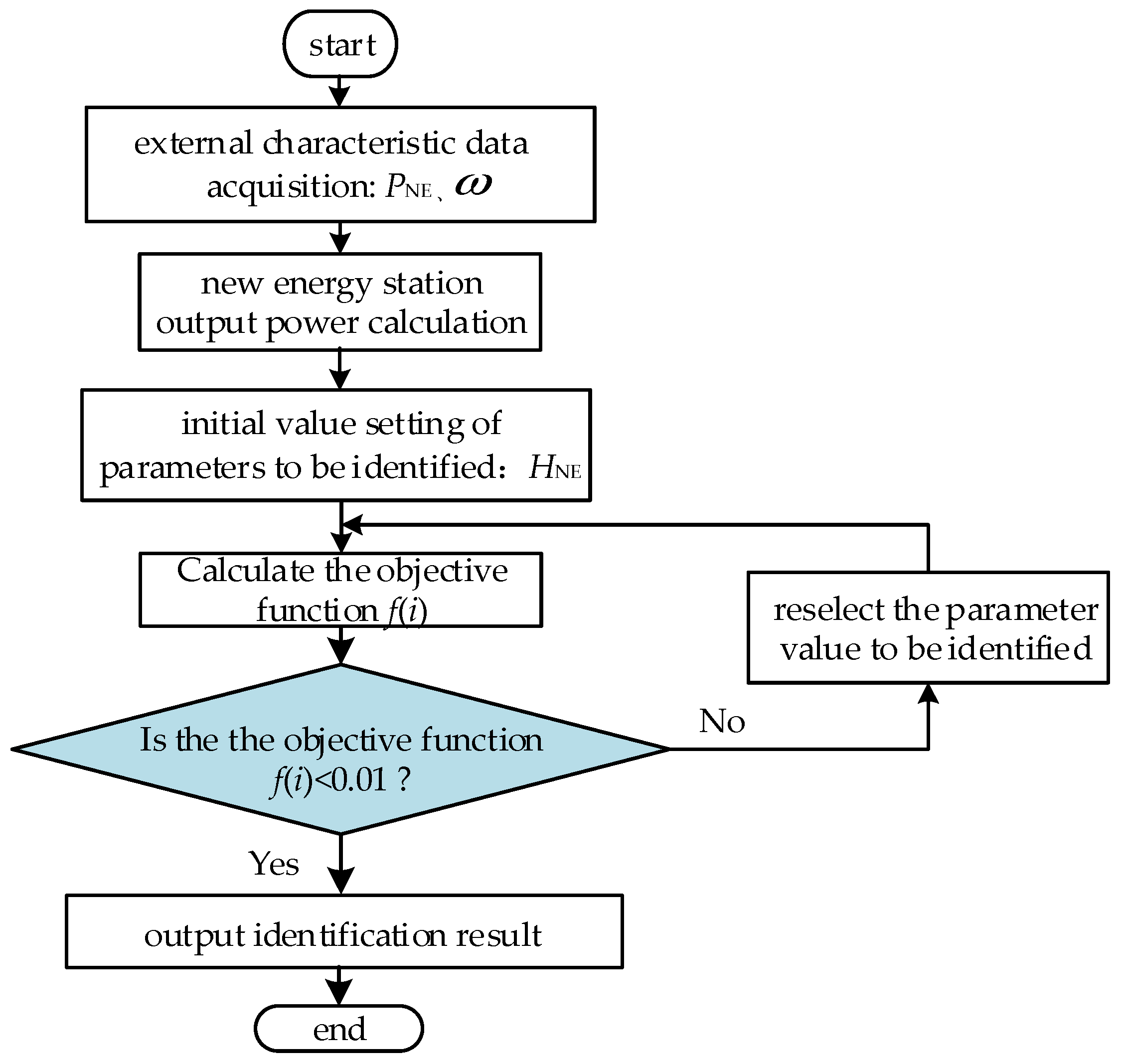
The steps for obtaining the H_NE of the renewable energy station using the genetic algorithm search are shown in Figure 6.

3.2. Calculation of the Point at which the Lowest Frequency Occurred

To obtain the analytical expression for the calculation of the lowest point of the frequency, a simplification was made to the G-ASF model: the time from the disturbance to the lowest point of the frequency is very short; therefore, a linear frequency deviation was introduced to simulate the frequency drop in the first few seconds, and a constant slope was used to simulate the overall response of the speed control system to the system power deficit:

$$\Delta P_{\mathrm{m}}=\frac{P_{\mathrm{d}}}{t_{\mathrm{nadir}}}t,t\in [0,t_{\mathrm{nadir}}].$$

(13)

In the formula, P_d is the power deficit, t_nadir is the moment at which the maximum frequency deviation occurs, and ΔP_m is the total increase in the mechanical power of the speed control system.

According to the swing equation of the rotor,

$$2H_{\mathrm{sys}}\frac{\mathrm{d}\Delta f(t)}{\mathrm{d}t}=\Delta P_{\mathrm{m}}(t)-\Delta P_{\mathrm{e}}(t).$$

(14)

In the formula, ΔP_e is the variation in the electromagnetic power.

Substituting Formula (13) and ΔP_e = P_d into Formula (14), we obtain

$$\frac{\mathrm{d}\Delta f(t)}{\mathrm{d}t}=\frac{P_{\mathrm{d}}}{2H_{\mathrm{sys}}}(\frac{t}{t_{\mathrm{nadir}}}-1).$$

(15)

The time-domain expression of the approximate frequency offset can be obtained by integrating Equation (15):

$$\Delta f(t)=\frac{P_{\mathrm{d}}}{2H_{\mathrm{sys}}}(\frac{1}{2t_{\mathrm{nadir}}}{t}^2-t).$$

(16)

In the formula, time t is an unknown variable, and t_nadir is an unknown constant.

Based on the time-domain expression of the frequency offset by the parabola approximation, the total primary frequency response of the system is obtained as follows [19]:

$$\begin{array}{ll}{P}_{\mathrm{PFR},\mathrm{sys}}(s)& =-G_{\mathrm{sys}}(s)\Delta f(s)\\ & =-\frac{P_{\mathrm{d}}}{2H_{\mathrm{sys}}}[\frac{1}{t_{\mathrm{nadir}}}\cdot \frac{G_{\mathrm{sys}}(s)}{s^3}-\frac{G_{\mathrm{sys}}(s)}{s^2}]\end{array},$$

(17)

where G_sys(s) is the equivalent primary frequency response transfer function of the system, namely,

$$G_{\mathrm{sys}}(s)=G_K(s)+G_{1-K}(s).$$

(18)

In the formula, G_K(s) is the total equivalent transfer function of the generator speed control system, and G_1−K(s) is the total equivalent transfer function of the renewable energy station; specifically,

$$G_{\mathrm{sys}}(s)={\displaystyle \sum _{i=1}^{N_G}{\alpha }_i{G}_i(s)}+{\displaystyle \sum _{j=N_G+1}^N{\alpha }_j{G}_j(s)}.$$

(19)

In the formula, G_i(s) is the transfer function of the low-order general speed control system of generator i, and G_j(s) is the transfer function of the general frequency response model of the renewable energy station j.

Substituting Equation (19) into Equation (17) and performing the inverse Laplace transform, P_PFR,sys can be obtained. In addition, because P_PFR,sys is equal to P_d when the frequency reaches the lowest point, we have

$$P_{\mathrm{PFR},\mathrm{sys}}(t_{\mathrm{nadir}})={\displaystyle \sum _{i=1}^{N_{\mathrm{G}}}{\alpha }_i{P}_{\mathrm{PFR},i}}(t_{\mathrm{nadir}})=P_{\mathrm{d}}.$$

(20)

The time at which the lowest point occurs, t_nadir, can be obtained by substituting the actual power deficit P_d into Formula (20); then, this was substituted into Formula (16) to obtain the frequency analysis formula Δf(t). We calculate the extreme value of Δf(t), and the lowest point of the frequency f_nadir can be obtained as

$$f_{\mathrm{nadir}}=(1-\frac{P_{\mathrm{d}}}{4H_{\mathrm{sys}}}{t}_{\mathrm{nadir}})f_0.$$

(21)

In the formula, f₀ is the base frequency 50 Hz.

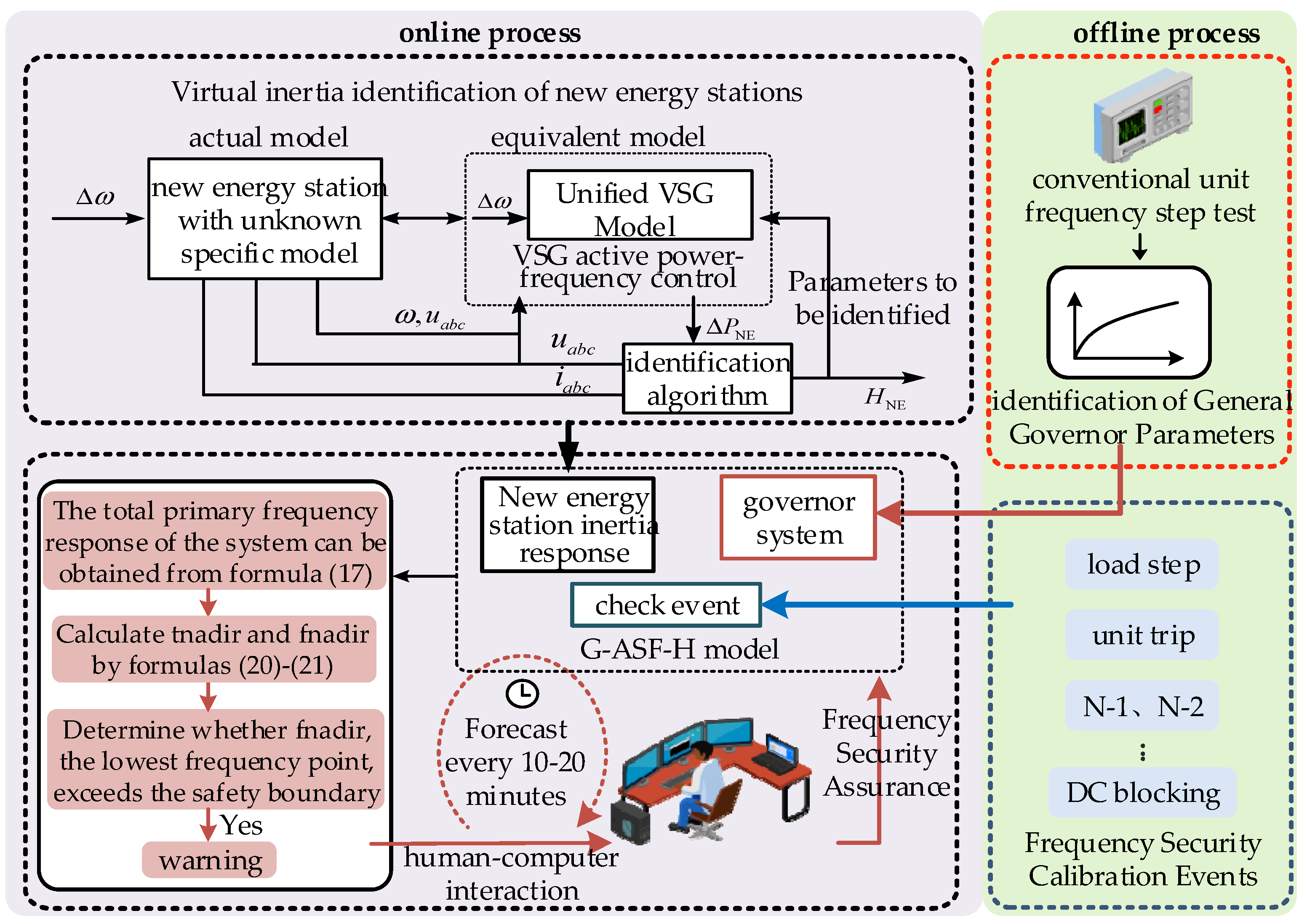
3.3. Online Security Assessment

Figure 7 shows the flowchart for the application of the G-ASF-H model to the online frequency security assessment. First, the frequency step test of the speed control system was performed offline to obtain the mechanical power response curve, thereby identifying the parameters of the general speed control system and avoiding the repeated analysis of the speed control system during operation. At the same time, events are also very important for frequency safety assessment. Offline predefinition of frequency safety verification events should include emergencies that have a large impact on the system frequency stability, which can be a 3% to 10% load step, bulk infeed HVDC system, generator trip, or typical N-1 or N-2 events, such as an active power deficit [28,29].

When running online, we measured the real-time power grid data, including the power output P_NE of the renewable energy stations and the grid frequency ω, and identified the virtual inertial time constant H_NE in real time. Based on the real-time data and the offline pre-stored speed control system parameters, we used the G-ASF-H model to obtain the lowest frequency point under predetermined emergency events.

To further improve the accuracy of the frequency safety assessment, a critical accident event at a certain moment was defined, under which we have

$$f_{\min }-\epsilon <f_{\mathrm{nadir}}<f_{\max }+\epsilon .$$

(22)

Here, f_nadir is the point at which the lowest frequency occurs, obtained using the G-ASF-H model; f_min and f_max are the frequency deviations in the power grid under large disturbances (a category of abnormal condition) not exceeding ±1.0 Hz, respectively; ε is the frequency boundary error.

If the frequency deviation exceeds the preset value, indicating an emergency, a warning is issued. The results of the online frequency security assessment are provided to operators for reference. If there are any critical or dangerous events, they can be simulated, and the results can be used for preventive control.

4. Case Analysis

To verify the effectiveness and accuracy of the renewable energy unit inertia identification method and the minimum frequency point calculation method proposed above, a simulation model of an IEEE system with 10 machines and 39 nodes was built using the PSCAD/EMTDC platform. The system topology is shown in Figure 8.

The system included seven conventional generators (G1~G7) and three wind farms (WF1~WF3), of which the rated capacities of the wind farms were 300 MVA, 600 MW, and 600 MW, respectively; the hydraulic turbine G1 was equipped with an IEEE G3 speed control system with a rated capacity of 1000 MVA, the steam turbines G2~G7 were equipped with an IEEE G1 speed control system, the rated capacity was 500 MVA, the total initial load of the system was 6192.8 MW, and the generator parameters are shown in

Table 1. Generator parameters for the 10-machine 39-node IEEE system.

Generator Type	Number	Output Power/MW	Inertial Time Constant/s
water turbine	G1	1000	10
steam turbine	G2	572.8	6.06
	G3	650	7.16
	G4	632	5.72
	G5	508	5.2
	G6	650	6.96
	G7	830	6.9
wind farm	WF1	250	4~10
	WF2	540	4~10
	WF3	560	4~10

.

4.1. H_NE Identification of Renewable Energy Stations and Calculation and Verification of the Point at which the Lowest Frequency Occurred

In this scenario, the initial power of the system was fixed at 0.8 p.u, and the virtual inertia time constant H_NE of the wind farm was set to 10 s. At this time, the number of variables contained in the individual in the genetic algorithm population was 1. Corresponding to the parameter H_NE to be identified, the proposed genetic algorithm was used to identify the H_NE of each wind farm. The relative error between the identification result and the actual value is shown in

Table 2. Comparison between the identification value of H_NE and the simulated value.

	HWF1	HWF2	HWF3
identification result	10.156	10.074	10.058
actual value	10	10	10
relative error	1.56%	0.74%	0.58%

.

From the identification value, the actual value, and the relative error of the virtual inertia time constant of each wind farm in Table 2, it can be seen that the error was within 2%, which verified the accuracy of the U-VSG model identification method.

On the basis of the identification of the H_NE of the wind farm, the accuracy of the G-ASF-H model under different disturbances was further studied. Figure 9 is a comparison chart between the actual frequency response (curve) of the system and the calculated value (red circle) of the proposed minimum point frequency prediction method after applying different disturbances. The maximum disturbance in the figure is 0.05 p.u, the minimum disturbance is 0.02 p.u, and the disturbance difference between the curves is 0.005 p.u. Figure 10 is a comparison chart between the actual frequency response (curve) of the system and the calculated value (red circle) of the proposed minimum point frequency prediction method under different load increments.

Under the condition that the initial load of the system remained unchanged and the disturbance load of the system increased,

Table 3. The comparison results of the calculated value and the simulated value of the lowest point.

Disturbance Load	Actual Value	Calculated Value	Error/%
120 MW	49.736	49.726	3.79%
150 MW	49.670	49.660	3.03%
180 MW	49.603	49.591	3.02%
210 MW	49.536	49.523	2.80%
240 MW	49.468	49.455	2.45%
270 MW	49.401	49.387	2.35%
300 MW	49.333	49.319	1.40%

shows the comparison results and relative errors between the actual value and the predicted value at the lowest point of each curve in Figure 9. Under different load increments, the error between the calculated value and the simulated value did not exceed 4%, as shown in Figure 10. It can be seen that under different disturbances, the prediction error of the proposed method was within 4%, and it can accurately predict the lowest point of the frequency under large disturbances.

4.2. Online Frequency Security Assessment Verification

To further verify the accuracy of the proposed calculation method in actual operation scenarios, we took the typical daily load curve of the actual power grid in a certain area as a reference. We selected 96 points in the daily load data of a certain day and calculated the lowest frequency point of each point in the case of the system load step; the load increase range was 120 MW, and the maximum load was set to 95% of the total power generation. Figure 11 shows the daily load curve and the virtual inertial time constants corresponding to the renewable energy stations at different times. Figure 12 shows the frequency response of the system when considering the time-varying characteristics of the virtual inertia of the new energy station and not considering the time-varying characteristics. It can be seen that considering the time-varying characteristics of the virtual inertia of new energy stations makes it possible to better reflect the frequency response process of the actual system after a disturbance.

Table 4. Renewable energy inertia H_NE identification results at different times.

Time	Actual Value	HWF1	HWF2	HWF3	Maximum Relative Error %
0:00	4	4.027	4.021	4.036	0.9
3:00	4	4.049	4.019	4.058	1.45
6:00	4	4.067	4.024	4.039	1.68
9:00	10	10.151	10.07	10.058	1.51
12:00	6	6.023	6.034	6.087	1.45
15:00	10	10.079	10.116	10.108	1.16
18:00	10	10.098	10.164	10.086	1.64
21:00	6	6.086	6.079	6.052	1.43

shows the identification results of the virtual inertial time constants of each renewable energy station every three hours over a day. The analysis shows that the maximum error in the different periods was not more than 2%, and the proposed H_NE identification method based on the genetic algorithm had high accuracy.

Figure 13 shows the calculation error distribution of the minimum frequency point at different times under the daily load curve for the G-ASF-H model considering the time-varying characteristics of the virtual inertia. It can be seen from the figure that the calculation error of less than 3% accounted for about 22.9%, the calculation error of 3–6% accounted for about 70.8%, and the calculation error of 6–9% accounted for about 6.3%. The results show that the proposed calculation method could accurately give the lowest frequency point of each point, and the maximum error did not exceed 9%. It can be seen from this example that the proposed method is suitable for online frequency security assessment.

5. Conclusions

Considering the time-varying characteristics of the virtual inertia of renewable energy stations under actual engineering conditions, in this paper, a G-ASF-H model was proposed for the prediction of the point at which the lowest frequency occurred and the realization of online safety assessments of the frequency following system disturbances. The main work was as follows:

(1) Based on the unified VSG model, the genetic algorithm was used to identify the parameters of the virtual inertia H_NE of the renewable energy station. The identification results of the parameters ensure that the output of the VSG model is consistent with the actual system, and that the accuracy is high.

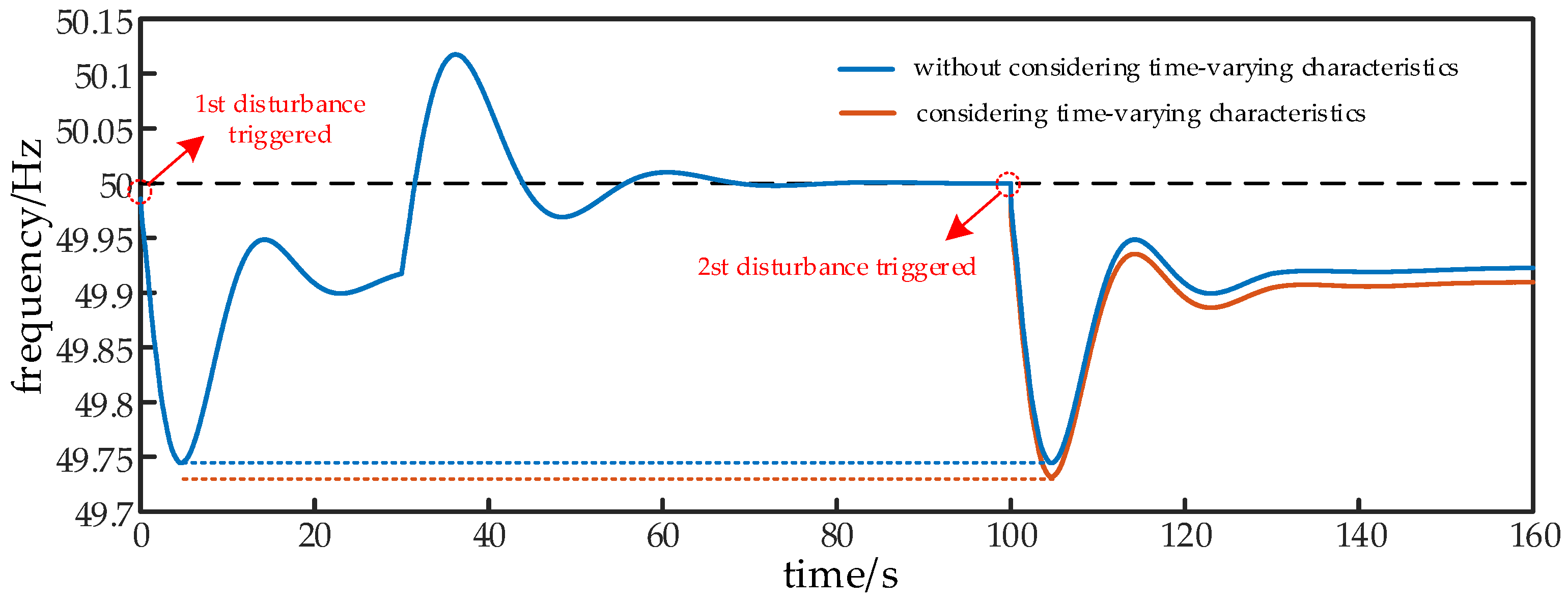
(2) The G-ASF-H model, which takes into consideration the time-varying characteristics of the virtual inertia of renewable energy stations, was proposed. Through the real-time identification of the virtual inertia H_NE of the renewable energy station, the problem of large error in the prediction results of the point at which the lowest system frequency occurs resulting from the change in H_NE being neglected by the existing model is avoided.

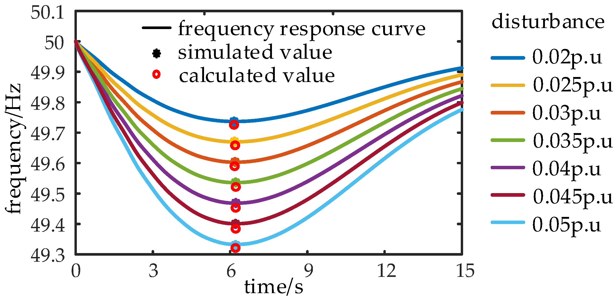
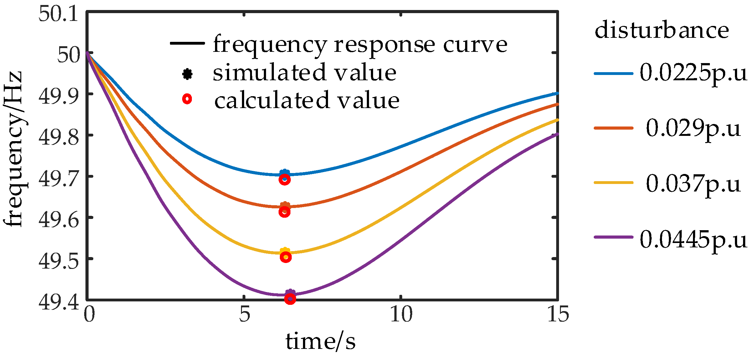
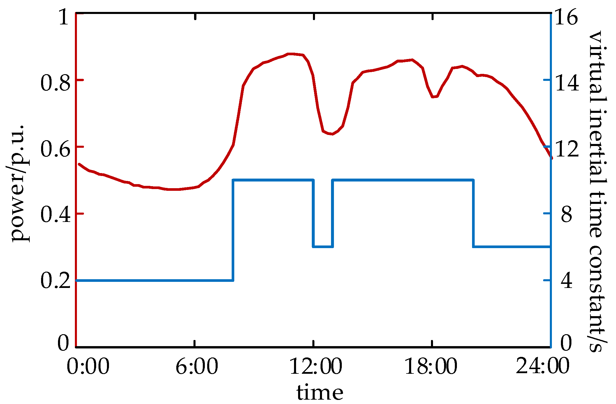
(3) Based on the proposed G-ASF-H model, which takes into consideration the time-varying characteristics of the virtual inertia of renewable energy stations, the accurate prediction of the point at which the lowest frequency occurs under different load disturbances and different daily load levels was realized, and can be further applied to the online security evaluation of system frequency.

In this paper, mainly the impact of deviations in transient frequency on the safe operation of the system was analyzed, and the indicators related to frequency safety included three aspects: steady-state frequency deviation, transient frequency deviation, and the frequency change rate. Combining multiple frequency security indicators to adjust the renewable energy output curve and frequency security assessment has certain significance for the actual power grid, and is one of the research directions of our future plans.