Self-Calibration for Sparse Uniform Linear Arrays with Unknown Direction-Dependent Sensor Phase by Deploying an Individual Standard Sensor

Abstract

Calibration of the unknown direction-dependent (DD) sensor phase and aliasing-free directions of arrival (DOA) estimation for sparse linear arrays are difficult tasks. In this work, we deploy an individual standard sensor with a known sensor phase response along the axis of the uncalibrated sparse linear array, a self-calibration method is proposed, in which the unknown DD sensor phase and the aliasing-free DOAs are both estimated. The proposed method is realized with a two-step scheme. In the first step, the sensor phase is eliminated by the Kronecker product of the covariance matrices in two different frequency bins, and the frequency difference satisfies the spatial Nyquist sampling theorem. Then, the DOAs can be robustly estimated without the influences of grating lobes and unknown sensor phase parameters. In the second step, the steering matrix is estimated with the known phase parameters of the deployed standard sensor. Then, the DD sensor phase is extracted from the steering matrix using the DOAs obtained in the first step. Hence, the disadvantages of iteration-based strategies in conventional calibration algorithms (e.g., local minima convergence) can be avoided. The performance of the proposed method is evaluated using simulation data and compared with that of Cramer–Rao bounds.

1. Introduction

Array signal processing techniques, such as the high-resolution direction-of-arrival (DOA) estimation [1,2] and adaptive beamforming [3], are sensitive to the unknown sensor responses. Calibration of sensor response is an important step to improve not only the DOA estimation but also the following adaptive beamformers: hydrophones ([4], Chapter 4), the fiber optic strain sensor [5] in an acoustic system, or antennas [6] in an electromagnetic system. Self-calibration is a type of calibration algorithm that can simultaneously estimate source DOA and array response vector parameters, such as coupling errors [7,8] and unknown sensor phase responses [9]. In applications such as speech or underwater acoustics, the bandwidth of the signals generated by speakers or sources typically exceeds 1 oct [10,11]. Accordingly, the half wavelength of the high frequency components is smaller than the interelement spacing, and the sensor array can be regarded as a sparse one. The coupling error between sensors can be ignored because of the large interelement spacing, whereas the unknown sensor phase occupies the array response mismatches.

Sensor phase responses can be modeled as direction-independent (DI) [11,12,13,14,15,16,17,18,19,20,21,22,23,24] or direction-dependent (DD) parameters [25,26,27]. Although numerous self-calibration methods for an unknown sensor phase have been proposed, most of them handle the DI sensor phase. The self-calibration methods for the DI model can be divided into two categories: self-calibration for the uncalibrated arrays and partly calibrated arrays. In the former, an iteration-based strategy is applied, and the sensor responses and DOAs are alternately estimated [12,13,14,15,16]. However, the iteration can easily converge to local minima due to poor initialization. In the latter category, partial sensor phase information is required beforehand [19,20,21,22,23], and DOAs and sensor responses are robustly estimated (e.g., ESPRIT-like algorithm) [19,20].

In contrast, it is difficult to distinguish whether the phase mismatch of the array response is caused by the DOA estimation errors or the unknown sensor phase under the DD model. Accordingly, the DOAs must first be obtained on the basis of the imperfect array response [24] or estimated with the partly calibrated sensors [23]. A DOA and steering vector estimation algorithm in [24] is a classical calibration algorithm for the DD sensor phase models. This algorithm alternately estimates the DOAs and the steering vectors with an iterative strategy. By contrast, the number of precalibrated sensors should be larger than that of sources to obtain the initial value of the DOAs, and the convergence heavily depends on the initializations. A weighted alternating least squares algorithm in [25] is also an iteration-based calibration algorithm for DD sensor parameters. The iteration easily converges to local minima due to the poor initialization. The instrumental sensor method in [26] is a noniterative algorithm that can estimate the DD sensor phase with instrumental sensors (i.e., precalibrated sensors). However, the number of precalibrated sensors should be also larger than that of the sources to make the unknown DOA and sensor responses solvable. In our previous work [27], the DD sensor phase parameters are extracted from the steering matrix without iterations. However, the DOAs should be first estimated with two precalibrated sensors.

These existing algorithms are not suitable for sparse uniform linear arrays (ULAs) because of the ambiguities in the spatial spectrum [28,29]. One disambiguation scheme for addressing this issue is to apply dual-size spatial invariance arrays; the ambiguous directions are eliminated with half-wavelength-spaced subarrays [30,31]. Another disambiguation scheme is the multistage DOA estimation scheme [32], in which the outputs of sensors are decomposed into multiple subbands and the influence of aliasing components is minimized due to the different structures of the aliasing components in each subband. However, the robustness against the unknown sensor response is not considered. To the authors’ knowledge, only a few studies have been conducted on self-calibration methods for sparse linear arrays.

This study proposes a self-calibration method for sparse ULAs with an unknown DD sensor phase. An individual standard sensor is first deployed along the axis of the sparse ULA. Then, a Kronecker product of covariance matrices in two different frequency bins is conducted. In this manner, the unknown and frequency invariant DD sensor phase is eliminated. Additionally, the frequency difference of the two different frequency bins satisfies the spatial Nyquist sampling theorem and the spatial aliasing is also avoided. The sensor phase is then calibrated with the constant modulus (CM) algorithm by using the estimated DOAs and the known phase response of the deployed standard sensor. In the proposed method, iterations are not required, and the disadvantages of iteration-based strategies in conventional calibration algorithms (e.g., local minima convergence) can be avoided. Moreover, the deployment of an additional standard sensor is easy to implement in real tasks.

2. Model Establishment

2.1. Sensor Phase Models

In this work, a ULA consisting of $M$ sensors with an unknown DD sensor phase is considered. We assume that the sensor phase response in the array does not have a uniform increment across the array but is frequency invariant [25] when processing low frequency signals, especially for hydrophones in sonar arrays ([4], Chapter 4). Thus, the direction-dependent sensor phase $\Phi$ can be modeled as follows:

$${\left[\Phi \right]}_{m,k}={\phi }_{m,k},$$

(1)

where ${\phi }_{m,k}$ is the phase response of the $m\mathrm{th}$ sensor in the direction of the $k\mathrm{th}$ signal.

A standard acoustic sensor with an accurate phase response is deployed along the axis of the uncalibrated ULA to calibrate the sensor phase parameters in the ULA. Thus, a new ULA with $M^{\prime }=M+1$ sensors is formed, and the deployed sensor becomes the first sensor in the new ULA, as shown in Figure 1. Without losing generality, we assume that the phase parameter of the deployed standard sensor is ${\phi }_{1,k}=0,k=1,\hspace{0.17em}\cdots ,K$, where $K$ is the number of signals.

2.2. Signal Model

K broadband and uncorrelated signals impinge on the ULA from the far field. The half wavelength of the incident signals is smaller than the interelement spacing, i.e., $\lambda /2<d$, where $d$ is the interelement spacing. Thus, the sensor array is regarded as the sparse ULA.

The sparse ULA and the deployed standard sensor synchronously acquire observation data. The observed time interval is partitioned into $L$ sections without overlapping. Then, a $Q$-point FFT is applied to each section. The frequency domain observation in the $l\mathrm{th}$ section and the $q\mathrm{th}$ frequency bin can be expressed as follows:

$$x_l(f_q)=\left[\begin{array}{c}{x}_{1,l}(f_q)\\ {x^{\prime }}_l(f_q)\end{array}\right]={\overline{A}}_q{s}_l(f_q)+\left[\begin{array}{c}{n}_{1,l}(f_q)\\ {n^{\prime }}_l(f_q)\end{array}\right],$$

(2)

where $x_{1,l}(f_q)$ and ${x^{\prime }}_l(f_q)$ are the observations of the deployed standard sensor and the original uncalibrated ULA, respectively; $s_l(f_q)={[s_{1,l}(f_q),\cdots ,s_{K,l}(f_q)]}^{\mathrm{T}}$ contains the signal spectra; and $n_{1,l}(f_q)$ and ${n^{\prime }}_l(f_q)={[n_{2,l}(f_q),\cdots ,n_{M^{\prime },l}(f_q)]}^{\mathrm{T}}$ are the additive Gaussian noise of the deployed standard sensor and the original uncalibrated ULA, respectively.

The steering matrix ${\overline{A}}_q$ in (2) is ${\overline{A}}_q=P\circ A_q$, where $P=e^{j\Phi }$; $A_q$ is the ideal steering matrix in the $q\mathrm{th}$ frequency bin; ${\left[A_q\right]}_{m,k}=\exp \left\{j2\pi f_q(m-1)d\cos {\theta }_k/c\right\}$, $m=1,2,\cdots ,M^{\prime }$, $c$ is the wave speed; ${\theta }_k$ is the unknown direction of the $k\mathrm{th}$ incident signal; and $\circ$ is the Hadamard product. Considering that ${\phi }_{1,k}=0,k=1,\cdots ,K$, we have ${\left[{\overline{A}}_q\right]}_{1,k}=1,k=1,\cdots ,K$.

On the basis of (2), the data covariance matrix in the $q\mathrm{th}$ frequency bin is represented as follows:

$$R_q=E\left\{x_l(f_q)x_l^{\mathrm{H}}(f_q)\right\}=(P\circ A_q){\Pi }_q{(P\circ A_q)}^{\mathrm{H}}+{\eta }_{q}I,$$

(3)

where ${\Pi }_q=\mathrm{diag}\left\{{\sigma }_q\right\}$, and ${\sigma }_q={[{\sigma }_{1,q},\cdots ,{\sigma }_{K,q}]}^{\mathrm{T}}$ denote the powers of the sources in the $q\mathrm{th}$ frequency bin, ${\eta }_q$ is the noise power in the $q\mathrm{th}$ frequency bin; $I$ is an $M^{\prime }\times M^{\prime }$ identity matrix, and ${(•)}^{\mathrm{H}}$ stands for the conjugate transpose.

In practice, the data covariance matrix $R_q$ is calculated from the sample covariance matrix as follows:

$${\widehat{R}}_q=\frac{1}{L}{\displaystyle \sum _{l=1}^L{x}_l(f_q)x_l^{\mathrm{H}}(f_q)},$$

(4)

where ${\widehat{R}}_q$ represents the sample covariance matrix.

3. Proposed Method

A robust DOA is first estimated without the influence of spatial aliasing or sensor phase uncertainties. Then, the sensor phase is calibrated using the estimated DOA values.

3.1. Robust DOA Estimation without Spatial Aliasing

Spatial aliasing is generated when the interelement spacing is larger than the half wavelength of the signal of interest (SOI). To overcome this issue, a frequency difference operation is conducted and the frequency of the SOI is pulled to a reference frequency $f_r$, which satisfies the spatial Nyquist sampling theorem (i.e., $f_r=c/(2d)$).

After the $Q$-point FFT operation, the index of the frequency bin for $f_r$ can be calculated as $q_r=\mathrm{round}\left\{Q{f}_r/f_s\right\}$, where $\mathrm{round}\{•\}$ is the rounding operation and $f_s$ is the sample rate.

Considering the properties of the Kronecker product, i.e., $\left(AB\right)\otimes \left(A^{\prime }{B}^{\prime }\right)=\left(A\otimes A^{\prime }\right)\left(B\otimes B^{\prime }\right)$, we can obtain the following expression:

$$\begin{array}{l}\left(R_q-{\eta }_{q}I\right)\otimes {\left(R_{q+q_r}^{}-{\eta }_{q+q_r}I\right)}^{\ast }=\left\{{\overline{A}}_q{\Pi }_q{\overline{A}}_q^{\mathrm{H}}\right\}\otimes {\left\{{\overline{A}}_{q+q_r}{\Pi }_{q+q_r}{\overline{A}}_{q+q_r}^{\mathrm{H}}\right\}}^{\ast }\\ =\left\{{\overline{A}}_q\otimes {\overline{A}}_{q+q_r}^{\ast }\right\}\left\{{\Pi }_q\otimes {\Pi }_{q+q_r}^{\ast }\right\}{\left\{{\overline{A}}_q\otimes {\overline{A}}_{q+q_r}^{\ast }\right\}}^{\mathrm{H}}\\ =B_{q,q+q_r}\mathrm{diag}\left\{{\sigma }_q\otimes {\sigma }_{q+q_r}\right\}{B}_{q,q+q_r}^{\mathrm{H}}\end{array},$$

(5)

where $\otimes$ is the Kronecker product, $\ast$ is the conjugate operation, and $B_{q,q+q_r}={\overline{A}}_q\otimes {\overline{A}}_{q+q_r}^{\ast }$.

In (5), the noise power ${\eta }_q$ and ${\eta }_{q+q_r}$ can be estimated by the average of the smallest $M^{\prime }-K$ eigenvalues of the sample covariance matrices ${\widehat{R}}_q$ and ${\widehat{R}}_{q+q_r}$, respectively, because the noise subspace estimation from the eigendecomposition of the sample covariance matrix is not affected by the unknown DD sensor phase.

The $((m_1-1)M^{\prime }+m_2)\mathrm{th}$ row and the $((k_1-1)K+k_2)\mathrm{th}$ column of matrix $B_{q,q+q_r}$ can be expressed as follows:

$$\begin{array}{l}{\left[B_{q,q+q_r}\right]}_{(m_1-1)M^{\prime }+m_2,(k_1-1)K+k_2}\\ =\exp \left\{j({\phi }_{m,{\overline{k}}_1}-{\phi }_{m,{\overline{k}}_2})\right\}\cdot \exp \left\{j\frac{2\pi }{c}\left[f_q(m_1-1)d\cos {\theta }_{{\overline{k}}_1}-f_{q+q_r}^{}(m_2-1)d\cos {\theta }_{{\overline{k}}_2}\right]\right\}\end{array},$$

(6)

where $1\le {\overline{k}}_1\le K$ and $1\le {\overline{k}}_2\le K$. Given the inconsistency of the order of the DOAs in ${\overline{A}}_q$ and ${\overline{A}}_{q+q_r}$, the $k_1\mathrm{th}$ column of the matrix ${\overline{A}}_q$ corresponds to the direction of the ${\overline{k}}_1\mathrm{th}$ signal and the $k_2\mathrm{th}$ column of the matrix ${\overline{A}}_{q+q_r}$ is the steering vector of the ${\overline{k}}_2\mathrm{th}$ signal.

When $m_1=m_2=m$, we have

$$\begin{array}{l}{\left[B_{q,q+q_r}\right]}_{(m-1)M^{\prime }+m,(k_1-1)K+k_2}=\exp \left\{j({\phi }_{m,{\overline{k}}_1}-{\phi }_{m,{\overline{k}}_2})\right\}\cdot \\ \exp \left\{-j\frac{2\pi }{c}{f}_r(m-1)d\frac{f_q\cos {\theta }_{{\overline{k}}_1}-f_{q+q_r}^{}\cos {\theta }_{{\overline{k}}_2}}{-f_r}\right\}\\ =\exp \left\{j({\phi }_{m,{\overline{k}}_1}-{\phi }_{m,{\overline{k}}_2})\right\}\cdot \exp \left\{-j\frac{2\pi }{c}{f}_r(m-1)d\cos {\overline{\theta }}_{{\overline{k}}_1,{\overline{k}}_2}\right\}\end{array},$$

(7)

where ${\overline{\theta }}_{{\overline{k}}_1,{\overline{k}}_2}=\arccos \left\{\left(f_q\cos {\theta }_{{\overline{k}}_1}-f_{q+q_r}^{}\cos {\theta }_{{\overline{k}}_2}\right)/\left(-f_r\right)+2\overline{k}\right\}$, and $\overline{k}$ is an integer that makes the inequality $\left|\left(f_q\cos {\theta }_{{\overline{k}}_1}-f_{q+q_r}^{}\cos {\theta }_{{\overline{k}}_2}\right)/\left(-f_r\right)+2\overline{k}\right|\le 1$ hold.

CASE I: ${\overline{k}}_1={\overline{k}}_2=k$

In this case, we have ${\theta }_{{\overline{k}}_1}={\theta }_{{\overline{k}}_2}={\theta }_k$. Thus, ${\overline{\theta }}_{{\overline{k}}_1,{\overline{k}}_2}$ is also equal to ${\theta }_k$, which is the direction of the $k\mathrm{th}$ signal. Given that $\exp \left\{j({\phi }_{m,{\overline{k}}_1}-{\phi }_{m,{\overline{k}}_2})\right\}=1$, the influence of the sensor phase is canceled. At this time, the steering matrix in (7) can be regarded as the equivalent steering matrix at the reference frequency in the direction of ${\theta }_k,k=1,\cdots ,K$. Considering that the reference frequency $f_r=c/(2d)$, the negative effect of the spatial aliasing is avoided.

CASE II: ${\overline{k}}_1\ne {\overline{k}}_2$

In this case, the direction of ${\overline{\theta }}_{{\overline{k}}_1,{\overline{k}}_2}$ is regarded as the cross term between the incident signals in ${\theta }_{{\overline{k}}_1}$ and ${\theta }_{{\overline{k}}_2}$. A total of $K^2-K$ cross terms are generated and ${\overline{\theta }}_{{\overline{k}}_1,{\overline{k}}_2},{\overline{k}}_1\ne {\overline{k}}_2$ varies with the frequency.

Then, we collect the $((m-1)M^{\prime }+m)\mathrm{th},m=1,\cdots ,M^{\prime }$ rows of $\left(R_q-{\eta }_{q}I\right)\otimes {\left(R_{q+q_r}^{}-{\eta }_{q+q_r}I\right)}^{\mathrm{H}}$ to form an equivalent covariance matrix at the reference frequency as follows:

$$\begin{array}{l}{\overline{R}}_{q,q+q_r}=J\left[\left(R_q-{\eta }_{q}I\right)\otimes {\left(R_{q+q_r}^{}-{\eta }_{q+q_r}I\right)}^{\mathrm{H}}\right]J^{\mathrm{H}}\\ =(J{B}_{q,q+q_r})\mathrm{diag}\left\{{\sigma }_q\otimes {\sigma }_{q+q_r}\right\}{({JB}_{q,q+q_r})}^{\mathrm{H}}\end{array},$$

(8)

where $J$ is an $M^{\prime }\times {M^{\prime }}^2$ section matrix with ${\left[J\right]}_{m,(m-1)M^{\prime }+m}=1$, and the other entries are equal to zero. The calculation of the equivalent covariance matrix at $f_r$ is shown in Figure 2.

Given the Kronecker product between ${\sigma }_q$ and ${\sigma }_{q+q_r}$ in (5), the number of signals (i.e., the incident signals and the cross terms) in the equivalent covariance matrix is $K^2$. The condition that $M^{\prime }>K^2$ should be satisfied to identify all the signals.

After the eigendecomposition of ${\overline{R}}_{q,q+q_r}$, we obtain unitary matrices ${\overline{U}}_{q,q+q_r}\in C^{M^{\prime }\times K^2}$ and ${\overline{V}}_{q,q+q_r}\in C^{M^{\prime }\times (M^{\prime }-K^2)}$, which are composed of signal and noise subspace eigenvectors, respectively. Similar to the traditional multiple signal classification algorithm (MUSIC), the spatial spectrum for the frequency pairs of $f_q$ and $f_{q+q_r}$ is estimated as follows:

$$P_q(\theta )=1/\left(b_r^{\mathrm{H}}{\overline{V}}_{q,q+q_r}^{}{\overline{V}}_{q,q+q_r}^{\mathrm{H}}{b}_r\right),$$

(9)

where ${\left[b_r\right]}_m=\exp \left\{-j2\pi f_r(m-1)d\cos \theta /c\right\}$.

In this spatial spectrum, the negative effects of the grating lobes and sensor phase uncertainties are avoided. However, the cross terms in Case II are the new interferences that degrade the DOA estimation performance of the incident signals. Given the sensor phase term (i.e., $e^{j({\phi }_{m,k_1}-{\phi }_{m,k_2})}$) in (7), the vector $b_r$ in (9) does not match $B_{q,q+q_r}$ in Case II. Consequently, the peaks of the cross terms are weaker than those of the incident signals. Additionally, the cross term ${\overline{\theta }}_{k_1,k_2},k_1\ne k_2$ varies with the frequency. These peaks are further weakened by the summation of $P_q(\theta )$ in the frequency domain:

$$P(\theta )={\displaystyle {\sum }_{q=q_L}^{q_H-q_r}{P}_q(\theta )},$$

(10)

where $q_L$ and $q_H$ are the lowest and highest frequency bins, respectively. According to Parseval’s theorem, the spatial spectrum $P(\theta )$ is also the power of the broadband signals.

3.2. DD Sensor Phase Calibration

We first apply the CM algorithm [27,28,33] to estimate the steering matrix in each frequency bin. Then, the DD sensor phase responses are extracted from the estimated steering matrix and the permutation problems are finally solved.

3.2.1. Steering Matrix Estimation

We assume that $U_q\in C^{M^{\prime }\times K}$ is the signal subspace of the covariance matrix $R_q$ through eigendecomposition. Thus, we have ${\overline{A}}_q=P\circ A_q=U_q{T}_q$, where $T_q$ is an $M^{\prime }\times M^{\prime }$ nonsingular matrix.

The norm of ${\left[{\overline{A}}_q\right]}_{m,k}$ can be written as follows:

$${\left|{\left[{\overline{A}}_q\right]}_{m,k}\right|}^2=t_{q(k)}^{\mathrm{H}}{u}_{q(m)}{u}_{q(m)}^{\mathrm{H}}{t}_{q(k)}=1,1\le m\le M^{\prime },$$

(11)

where $|•|$ is the modulus of a complex number, $u_{q(m)}^{\mathrm{H}}$ is the $m\mathrm{th}$ row of $U_q$, and $t_{q(k)}$ is the $k\mathrm{th}$ column of $T_q$.

Considering that the modulus of ${\left[{\overline{A}}_q\right]}_{m,k}$ is always equal to one for any indices of $m$ and $k$, we have

$$\begin{array}{l}{\left|{\left[{\overline{A}}_q\right]}_{m,k}\right|}^2-{\left|{\left[{\overline{A}}_q\right]}_{1,k}\right|}^2=t_{q(k)}^{\mathrm{H}}{K}_{q,m}{t}_{q(k)}\\ ={\mathrm{vec}}^{\mathrm{T}}(K_{q,m})\left(t_{q(k)}^{}\otimes t_{q(k)}^{\ast }\right)=0,m=2,\cdots ,M^{\prime }\end{array},$$

(12)

where $K_{q,m}=u_{q(m)}{u}_{q(m)}^{\mathrm{H}}-u_{q(1)}{u}_{q(1)}^{\mathrm{H}}$, and $\mathrm{vec}(•)$ is the matrix vectorization.

The $M^{\prime }-1$ equations in (12) are written in a matrix form as follows:

$$K_q\left(t_{q(k)}^{}\otimes t_{q(k)}^{\ast }\right)=0_{M-1},$$

(13)

where $0_{M-1}$ is $(M^{\prime }-1)\times 1$ vector with all elements equal to zero, and $K_q$ is an $(M^{\prime }-1)\times K^2$ matrix whose $(m-1)\mathrm{th}$ row is ${\mathrm{vec}}^{\mathrm{T}}(K_{q,m})$, $m=2,\cdots ,M^{\prime }$.

The vector $t_{q(k)}^{}\otimes t_{q(k)}^{\ast }$ belongs to the null space of $K_q$ (denoted as $\mathbb{N}\left\{K_q\right\}$). The null space $\mathbb{N}\left\{K_q\right\}$ can be calculated from the singular value decomposition of matrix $K_q$. If the right singular matrix of $K_q$ is $Z_q=[z_1,\cdots ,z_{K^2}]$ and $z_k$ is the $k\mathrm{th}$ right singular vectors of $K_q$, we find that $\mathbb{N}\left\{K_q\right\}=[z_{K^2-K+1},\cdots ,z_{K^2}]$.

In accordance with [27,33], $t_{q(k)}^{}\otimes t_{q(k)}^{\ast },k=1,\dots ,K$ is also a group of linearly independent vectors of $\mathbb{N}\left\{K_q\right\}$. Thus, any vector $w^q\in \mathbb{N}\left\{K_q\right\}$ can be expressed as follows:

$$\begin{array}{l}{w}^q={\displaystyle \sum _{t=1}^K{\alpha }_t^q{z}_{K^2-K+t}^{}}={\displaystyle \sum _{t=1}^K{\beta }_t^q\left(t_{q(t)}^{}\otimes t_{q(t)}^{\ast }\right)}\\ \Rightarrow W_q={\mathrm{vec}}^{-1}\left\{w^q\right\}={\left(T_q^T\right)}^{-1}{\Sigma }_q{T}_q^{\mathrm{T}}\end{array},$$

(14)

where ${\alpha }_t^q$ and ${\beta }_t^q$ are the coefficients under the different basis of null space $\mathbb{N}\left\{K_q\right\}$, ${\mathrm{vec}}^{-1}$ is the inverse operation of matrix vectorization, and ${\Sigma }_q=\mathrm{diag}\left\{{\beta }_1^q,\cdots ,{\beta }_K^q\right\}$.

If ${\Sigma }_q$ is a nonsingular matrix, then we obtain

$$W_q^{-1}{W^{\prime }}_q={\left\{T_q^{\mathrm{T}}\right\}}^{-1}\left({\Sigma }_q^{-1}{{\Sigma }^{\prime }}_q\right)T_q^{\mathrm{T}},$$

(15)

where ${{\Sigma }^{\prime }}_q=\mathrm{diag}\left\{{{\beta }^{\prime }}_1^q,\cdots ,{{\beta }^{\prime }}_K^q\right\}$, ${{\beta }^{\prime }}_t^q,t=1,\cdots ,K$ is another coefficient and ${{\beta }^{\prime }}_t^q\ne {\beta }_t^q$.

The version in (15) is similar to the eigendecomposition of the matrix $W_q^{-1}{W^{\prime }}_q$. Additionally, we can calculate the steering matrix ${\overline{A}}_q$ as follows by considering that ${\overline{A}}_q=U_q{T}_q$ and ${\left[{\overline{A}}_q\right]}_{1,k}=1,k=1,\cdots ,K$ [27]:

$${\widehat{\overline{A}}}_q={\tilde{A}}_q{\mathrm{diag}}^{-1}\left\{e_1^{\mathrm{T}}{\tilde{A}}_q\right\}{J^{\prime }}_q,$$

(16)

where ${\tilde{A}}_q=U_q{\left\{E_q^{\mathrm{T}}\right\}}^{-1}$, $E_q$ is the unitary matrix composed of the eigenvectors of $W_q^{-1}{W^{\prime }}_q$, ${J^{\prime }}_q=[e_{{n^{\prime }}_1},e_{{n^{\prime }}_2},\cdots ,e_{{n^{\prime }}_K}]$ is a $K\times K$ selection matrix, ${n^{\prime }}_1\ne {n^{\prime }}_2\ne \cdots \ne {n^{\prime }}_K$, ${n^{\prime }}_1,\cdots ,{n^{\prime }}_K\in \left\{1,2,\cdots ,K\right\}$, and $e_{{n^{\prime }}_k}$ is a vector with the ${n^{\prime }}_k\mathrm{th}$ element equal to one and with the other equal to zero. The arrangement of the columns of the steering matrix at different frequency bins is adjusted by the selection matrix ${J^{\prime }}_q$, which is calculated later.

3.2.2. Sensor Phase Estimation

In the $q\mathrm{th}$ frequency bin, we define

$${\overline{\psi }}_q=\mathrm{angle}\left\{{\overline{A}}_q\right\},{\psi }_q=\mathrm{angle}\left\{A_q\right\},$$

(17)

where $\mathrm{angle}\{•\}$ is the phase of the bracketed variable.

The relationship of the phase of the steering matrix can be expressed as follows:

$$\left\{\Phi +{\psi }_q{J^{″}}_q\right\}\mathrm{mod}(2\pi )={\overline{\psi }}_q,q=q_L,\cdots ,q_H,$$

(18)

where $a\mathrm{mod}b$ is the remainder of $a$ divided by $b$ and a selection matrix ${J^{″}}_q=[e_{{n^{″}}_1},e_{{n^{″}}_2},\cdots ,e_{{n^{″}}_K}]$; ${n^{″}}_1\ne {n^{″}}_2\ne \cdots \ne {n^{″}}_K$, ${n^{″}}_1,\cdots ,{n^{″}}_K\in \left\{1,2,\cdots ,K\right\}$ is introduced in (18) to align the sequence of the sensor phase responses between ${\overline{\psi }}_q$ and ${\psi }_q$. Then, we have

$$\Phi =\left\{{\overline{\psi }}_q-{\psi }_q{J^{″}}_q\right\}\mathrm{mod}(2\pi ),q=q_L,\cdots ,q_H,$$

(19)

The sensor phase is frequency invariant and can be estimated by averaging (19) along the frequency domain:

$${\widehat{\phi }}_{m,k}=\frac{1}{q_H-q_L+1}{\displaystyle \sum _{q=q_L}^{q_H}\left\{{\left[{\overline{\psi }}_q-{\psi }_q{J^{″}}_q\right]}_{m,k}\right\}\mathrm{mod}(2\pi )},$$

(20)

3.2.3. Permutation Problem Solving

Two permutation problems, namely, ${J^{\prime }}_q$ in (16) and ${J^{″}}_q$ in (19), need to be addressed.

To align the columns of the estimated steering matrix in (16) at different frequency bins, we calculate the selection matrix ${J^{\prime }}_q$ by minimizing the difference of the steering matrix at neighboring frequency bins as [27]

$$\begin{array}{l}{{\widehat{J}}^{\prime }}_q=\underset{{J^{\prime }}_q}{\min }{\Vert {\tilde{A}}_q{\mathrm{diag}}^{-1}\left\{e_1^{\mathrm{T}}{\tilde{A}}_q\right\}{J^{\prime }}_q-{\widehat{\overline{A}}}_{q-1}\Vert }_{\mathrm{F}},q=q_L+1,\cdots ,q_H\\ s.t.{\widehat{\overline{A}}}_{q_L}={\tilde{A}}_{q_L}{\mathrm{diag}}^{-1}\left\{e_1^{\mathrm{T}}{\tilde{A}}_{q_L}\right\}\end{array},$$

(21)

which means that ${\widehat{\overline{A}}}_q,q=q_L+1,\cdots ,q_H$ aligns with ${\widehat{\overline{A}}}_{q_L}$.

In (19), the selection matrix ${J^{″}}_q$ is used to align the sequence of the sensor phase responses between ${\overline{\psi }}_q$ and ${\psi }_q$. Given that the sensor phase response is frequency invariant, the variance of $\left\{{\overline{\psi }}_q-{\psi }_q{J^{″}}_q\right\}\mathrm{mod}(2\pi )$ along the frequency domain approaches zero for an appropriate ${J^{″}}_q$. Hence, ${J^{″}}_q$ can be calculated as follows:

$$\begin{array}{l}{{\widehat{J}}^{″}}_q=\underset{{J^{″}}_q}{\min }\mathrm{var}\left\{\upsilon \right\}\\ \upsilon =\frac{1}{MK}[{\displaystyle \sum _{k=1}^K{\displaystyle \sum _{m=1}^M\left\{{\left[{\overline{\psi }}_{q_L}-{\psi }_{q_L}{J^{″}}_{q_L}\right]}_{m,k}\right\}\mathrm{mod}(2\pi )}},\cdots ,{{\displaystyle \sum _{k=1}^K{\displaystyle \sum _{m=1}^M\left\{{\left[{\overline{\psi }}_{q_H}-{\psi }_{q_H}{J^{″}}_{q_H}\right]}_{m,k}\right\}\mathrm{mod}(2\pi )}}]}^{\mathrm{T}}\end{array},$$

(22)

where $\mathrm{var}\{•\}$ is the variance of the bracketed vector.

3.3. Algorithmic Steps

In the proposed method, the DOAs are first estimated without the influences of the unknown sensor phase and spatial aliasing. Then, the DD sensor phase is calibrated with the estimated DOAs. The algorithmic steps for the sparse ULA are described in

Table 1. Algorithmic steps in the proposed method.

Algorithm: Self-calibration for sparse ULAs with unknown DD sensor phase
Input: Phase parameters of the standard sensor, observations of the sparse ULA and the individual standard sensor Output: Estimated DOAs and the DD sensor phase responses of the sparse ULA
1:	$x_l(f_q)$ is obtained by the Q-point FFTs on the L sections of the array observations.
2:	The sample covariance matrix ${\widehat{R}}_q$ is calculated in (4).
3:	Noise power ${\eta }_q$ is calculated by averaging the small $M^{\prime }-K$ eigenvalues of the sample covariance matrix ${\widehat{R}}_q$.
4:	// Step 1 Estimate the DOAs
5:	Calculate the equivalent covariance matrix ${\overline{R}}_{q_1,q_1+q_r}$ in (8).
6:	The DOA for the frequency pairs of $f_{q_1}$ and $f_{q_1+q_r}$ is estimated in (9).
7:	The broadband spatial spectrum is calculated in (10).
8:	// Step 2 Estimate the DD sensor phase
9:	The steering matrix ${\widehat{\overline{A}}}_q$ is estimated in (16) and the selection matrix ${J^{\prime }}_q$ is calculated in (21).
10:	The sensor phase is estimated in (20) and the selection matrix ${J^{″}}_q$ is calculated in (22).

.

3.4. Discussions

3.4.1. Discussion on the Deployed Standard Sensors

Although an individual standard sensor is deployed in the previous derivation, we still need to discuss why the individual standard sensor is required in the proposed method.

Lemma 1.

At least one individual standard sensor is required to calibrate the DD sensor phase.

Proof. 

After deploying an individual standard sensor along the axis of the original uncalibrated sparse ULAs, a new ULA is formed and the deployed standard sensor becomes the first sensor of the new ULA. In accordance with (16), the estimated steering matrix is normalized by the first row of the matrix ${\tilde{A}}_q$. If the phase responses of the first sensor (i.e., the deployed standard sensor) are symbolized as ${{\phi }^{\prime }}_{1,•}={[{{\phi }^{\prime }}_{1,1},{{\phi }^{\prime }}_{1,2},\cdots ,{{\phi }^{\prime }}_{1,K}]}^{\mathrm{T}}$, then the estimated steering matrix can be expressed as follows:

$$\begin{array}{l}{{\widehat{\overline{A}}}^{\prime }}_q={\tilde{A}}_q{\mathrm{diag}}^{-1}\left\{e_1^{\mathrm{T}}{\tilde{A}}_q\right\}\mathrm{diag}\left\{e^{j{{\phi }^{\prime }}_{1,•}}\right\}{J^{\prime }}_q\\ ={\tilde{A}}_q^{norm}\mathrm{diag}\left\{e^{j{{\phi }^{\prime }}_{1,•}}\right\}{J^{\prime }}_q\end{array},$$

(23)

where ${\tilde{A}}_q^{norm}={\tilde{A}}_q{\mathrm{diag}}^{-1}\left\{e_1^{\mathrm{T}}{\tilde{A}}_q\right\}$.

If ${{\phi }^{\prime }}_{1,•}$ can be estimated, then the deployed sensor phase parameter is not necessary. In other words, specifically, no deployed sensor is required. However, if ${{\phi }^{\prime }}_{1,•}$ cannot be identified, at least one deployed sensor is needed.

The covariance matrix reconstructed by the steering matrix ${{\widehat{\overline{A}}}^{\prime }}_q$ is represented as

$$\begin{array}{l}{R^{\prime }}_q={{\widehat{\overline{A}}}^{\prime }}_q{\Pi }_q{{\widehat{\overline{A}}}^{\prime }}_q^{\mathrm{H}}+{\eta }_{q}I\\ ={\tilde{A}}_q^{norm}\mathrm{diag}\left\{e^{j{{\phi }^{\prime }}_{1,•}}\right\}{J^{\prime }}_q{\Pi }_q{\left({J^{\prime }}_q\right)}^{\mathrm{H}}{\mathrm{diag}}^{\mathrm{H}}\left\{e^{j{{\phi }^{\prime }}_{1,•}}\right\}{\left({\tilde{A}}_q^{norm}\right)}^{\mathrm{H}}+{\eta }_{q}I\\ ={\tilde{A}}_q^{norm}\mathrm{diag}\left\{e^{j{{\phi }^{\prime }}_{1,•}}\right\}\mathrm{diag}\left\{{J^{\prime }}_q{\sigma }_q\right\}{\mathrm{diag}}^{\mathrm{H}}\left\{e^{j{{\phi }^{\prime }}_{1,•}}\right\}{\left({\tilde{A}}_q^{norm}\right)}^{\mathrm{H}}+{\eta }_{q}I\\ ={\tilde{A}}_q^{norm}\mathrm{diag}\left\{e^{j{{\phi }^{\prime }}_{1,•}}\circ \left({J^{\prime }}_q{\sigma }_q\right)\circ {\left(e^{j{{\phi }^{\prime }}_{1,•}}\right)}^{\mathrm{H}}\right\}{\left({\tilde{A}}_q^{norm}\right)}^{\mathrm{H}}+{\eta }_{q}I\end{array},$$

(24)

In consideration of the commutativity of the Hadamard product, Equation (24) can be reformed as

$$\begin{array}{l}{R^{\prime }}_q={\tilde{A}}_q^{norm}\mathrm{diag}\left\{e^{j{{\phi }^{\prime }}_{1,•}}\circ {\left(e^{j{{\phi }^{\prime }}_{1,•}}\right)}^{\mathrm{H}}\circ \left({J^{\prime }}_q{\sigma }_q\right)\right\}{\left({\tilde{A}}_q^{norm}\right)}^{\mathrm{H}}+{\eta }_{q}I\\ ={\tilde{A}}_q^{norm}\mathrm{diag}\left\{{J^{\prime }}_q{\sigma }_q\right\}{\left({\tilde{A}}_q^{norm}\right)}^{\mathrm{H}}+{\eta }_{q}I\\ ={\tilde{A}}_q^{norm}{J^{\prime }}_q\mathrm{diag}\left\{{\sigma }_q\right\}{\left({\tilde{A}}_q^{norm}{J^{\prime }}_q\right)}^{\mathrm{H}}+{\eta }_{q}I\\ ={\widehat{\overline{A}}}_q{\Pi }_q{\widehat{\overline{A}}}_q^{\mathrm{H}}+{\eta }_{q}I\end{array},$$

(25)

where ${\widehat{\overline{A}}}_q$ is the steering matrix defined in (16). □

According to (25), the deployed sensor phase response ${{\phi }^{\prime }}_{1,•}$ is canceled, indicating that the variable ${{\phi }^{\prime }}_{1,•}$ cannot be identified from the covariance matrix. Hence, at least one deployed standard sensor with known phase response is required to estimate the unknown sensor phase responses of the original uncalibrated ULA.

3.4.2. Comparison with the Current Self-Calibration Algorithms

In the current self-calibration algorithms, an iteration-based strategy is commonly used, in which the DOAs and sensor phase are alternatively estimated during the iterations [12,13,14,15,16]. However, the local minima are easily converged due to the poor initialization. The initializations of the DOAs are difficult to choose, especially for the sparse linear arrays, because of the spatial aliasing.

To avoid the disadvantages of the iteration strategy, the self-calibration method in [27] and the proposed method both work without iterations. In [27], the DOAs are first obtained from the estimated steering matrix with two precalibrated sensors and the DD sensor phase is then calculated. The DOA estimation accuracy is significantly influenced by the number of the precalibrated sensors. The estimation of the DD sensor phase is also limited. Moreover, the assumption of the multiple precalibrated sensors that belong to the uncalibrated array is unrealistic in practice.

By contrast, the DOA estimation accuracy of the proposed method is improved owing to the use of the whole aperture of the sensor array and elimination of the unknown sensor phase. Additionally, spatial aliasing is no longer a problem when the proposed method is applied to the sparse ULAs since it is based on the frequency difference methodology. Notably, only an additional standard sensor is exploited for the extraction of the sensor phase, which is easier to implement in real tasks since the sensor is not a part of the original uncalibrated array.

4. Simulation Results

A sparse ULA composed of 11 acoustic sensors is considered in the simulation. The wave speed in the water medium is 1500 m/s. The interelement spacing is equal to 3.75 m (i.e., the half wavelength of 200 Hz). Two uncorrelated broadband signals impinge on the array from the directions of 50° and 80°, respectively, and they cover the frequency band from 200 to 600 Hz. The test array is sparse relative to the frequency band of the incident signals.

A standard sensor is deployed along the axis of the sparse ULA and a new ULA with $M^{\prime }=12$ sensors is formed. The deployed sensor now becomes the first sensor of the new ULA. The accurate sensor phase of the deployed sensor and the unknown sensor phase responses, which are frequency invariant and randomly generated from uniform distributions in the range $-\pi ~\pi$, are listed in

Table 2. Sensor phase responses.

DOAs	m	1	2	3	4	5	6
50°	$\phi$ (rad)	0.0000	−1.2865	0.8886	0.8369	−1.5832	1.5472
80°	$\phi$ (rad)	0.0000	−0.8488	2.0270	−1.1582	0.0490	−0.2114
	m	7	8	9	10	11	12
50°	$\phi$ (rad)	2.2316	0.9938	1.2671	0.4506	1.8271	0.4833
80°	$\phi$ (rad)	1.9140	0.5766	−1.4600	0.0922	1.8587	−2.1943

. The sample frequency is set to 5 kHz.

4.1. Example for DOAs and DD Sensor Phase Estimation

The observed data are partitioned into $L=200$ sections, with each section containing 500 samples. A $Q$-point FFT is applied to each section, and $Q=500$. A total of 41 frequency bins are located in the frequency band. We set the reference frequency $f_r=200\mathrm{Hz}$ to avoid spatial aliasing. SNR is set to 5 dB. In the proposed method, the first sensor is assumed to be precalibrated.

The spatial spectra of the proposed method with $f_q=200,250,300,350,\mathrm{and}400\mathrm{Hz}$ (i.e., Equation (9)) and the broadband (i.e., Equation (10)) are plotted in Figure 3a. The spectral values of the cross terms are much lower than the peaks of the incident signals due to the mismatch between $b_r$ in (9) and $B_{q_1,q_1+q_r}$ in (7). Hence, two sharp peaks can be observed in all the spatial spectra in Figure 3a. After summing the spatial spectra along the frequency domain, we observe that the broadband spectrum has relatively flat sidelobe sectors. Additionally, spatial aliasing is effectively avoided.

The unknown DD sensor phase parameters are then obtained by applying the estimated DOAs. The true and the estimated sensor phase values are displayed in Figure 3b. We can observe that the proposed method shows a high estimation accuracy of the DD sensor phase.

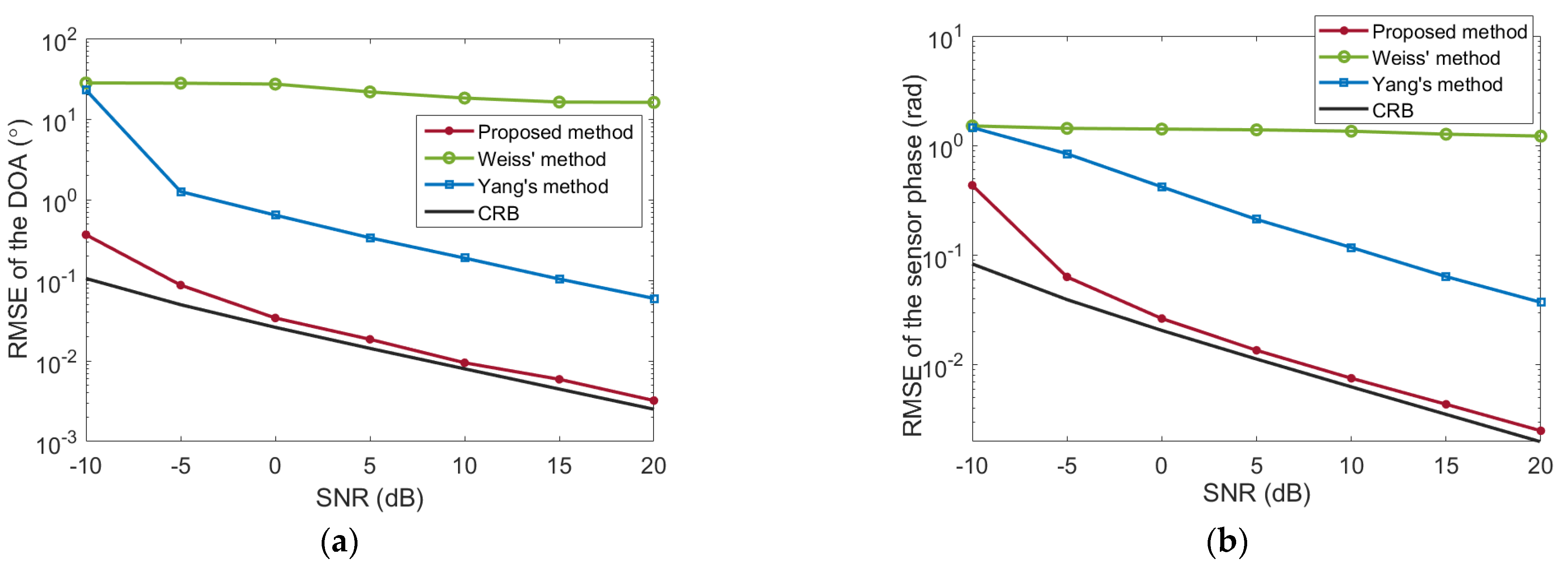
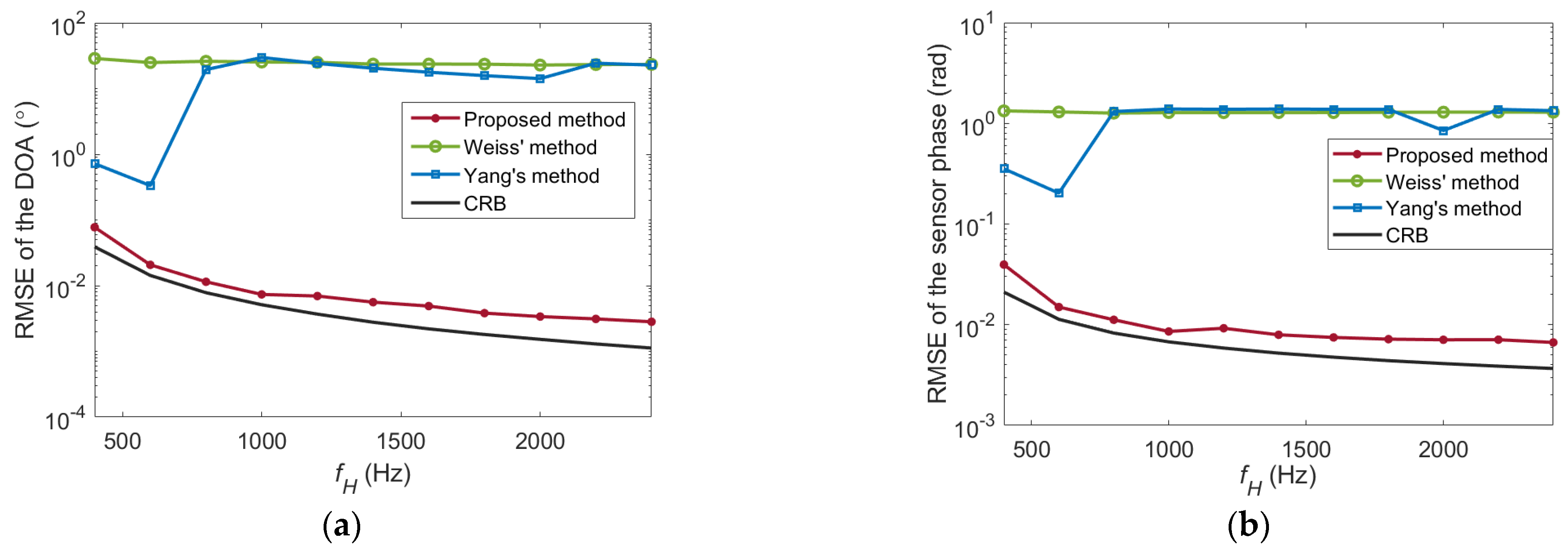
4.2. Statistical Performance of the Proposed Algorithm

The statistical performance of the proposed algorithm is shown in the following simulation. Considering that studies on the self-calibration of the unknown DD sensor phase are limited, Weiss’ method in [25], Yang’s method in [27], and the Cramer–Rao bounds (CRBs) [25,27] are applied for comparison. In Weiss’ method, the number of precalibrated sensors is set to three. Yang’s method requires two precalibrated sensors. In addition, the Weiss’ method is a narrowband processing algorithm that is applied in each frequency bin and the sensor phase parameters and the DOAs are averaged over the frequency band. The estimates of DOAs and sensor phase responses are measured by the root mean square error (RMSE). A total of 200 Monte Carlo experiments are conducted.

The statistical performance of the estimates of the DOAs and sensor phase responses versus the SNR are shown in Figure 4a,b, respectively. In Weiss’ method, the low estimation accuracy of the DOAs and sensor phase parameters is caused by the poor initialization of the DOAs resulting from the spatial aliasing and the short aperture of the precalibrated subarray. Yang’s method can calibrate the sensor phase responses whose performance is also affected by the directions of the sources. In Yang’s method, the DOAs are estimated with the first two precalibrated sensors at an equivalent frequency of $\left(f_{\mathrm{H}}-f_{\mathrm{L}}\right)/2$ [27]. At this equivalent frequency, the spatial ambiguity can be avoided, whereas the estimation accuracy of the DOAs is still limited by the aperture of the first two precalibrated sensors. The proposed method has the best DOA estimation performance among the methods mainly because of the applications of the whole aperture of the sensor array and the anti-aliasing processing. The calibration performance of the sensor phase responses is also improved owing to the unambiguous and accurate DOAs. The CRBs of the DOA and sensor phase estimation in Figure 4a,b are also well approached by the proposed method.

We repeat the simulation by fixing SNR = 5 dB and varying the number of sections L from 20 to 300. Each section also contains 500 samples. The estimation performance of DOAs and sensor phase responses versus the number of sections are shown in Figure 5a,b, respectively. Similar to the results in Figure 4, the proposed method has the lowest RMSE values among the compared methods, and the CRB is approached.

In the next simulation, the effect of the signal bandwidth on the performance of the mentioned self-calibration algorithms is discussed. We fix the lower limit frequency of the incident signals $f_{\mathrm{L}}$ as 200 Hz, whose wavelength is equal to twice the interelement spacing. Additionally, the higher limit frequency $f_{\mathrm{H}}$ ranges from 400 to 2400 Hz at a step of 200 Hz, indicating that the bandwidth of the incident signals increases from 1 oct to approximately 3.5 oct. The larger the $f_{\mathrm{H}}$, the sparser of the sensor array. Additionally, SNR is set to 5 dB, and the number of sections $L=200$.

The RMSEs of the DOAs and sensor phase responses versus the signal bandwidth are plotted in Figure 6a,b, respectively. Weiss’ method fails to estimate the unknown parameters. In Yang’s method, the equivalent frequency of $\left(f_{\mathrm{H}}-f_{\mathrm{L}}\right)/2$ does not satisfy the spatial Nyquist sampling theorem when the higher limit frequency $f_{\mathrm{H}}$ is larger than 600 Hz. Accordingly, the estimation performance is dramatically degraded due to the spatial ambiguity for $f_{\mathrm{H}}>600\mathrm{Hz}$. However, the directions of the sources are estimated at the reference frequency, and the spatial Nyquist sampling theorem is always satisfied in the proposed method. Moreover, the DOA estimation performance can be improved with more frequency bins applied due to the increased signal bandwidth. The RMSE of the proposed method is also approached by the CRB.

5. Conclusions

A self-calibration method is proposed by deploying an individual standard sensor with a known sensor phase response along the axis of the uncalibrated sparse linear array, in which the unknown DD sensor phase and the aliasing-free DOAs are estimated. The DOA is first accurately estimated owing to the use of the whole aperture of the sensor array and the elimination of unknown sensor phase. Additionally, spatial aliasing is also solved based on the frequency difference methodology. Then, the steering matrix is estimated by the CM algorithm with the known phase parameters of the deployed standard sensor. The DD sensor phase is finally extracted from the steering matrix by using the estimated DOAs.

The advantages of the proposed method are summarized as follows: (1) The DOAs can be accurately estimated even if the sensor phase is unknown. (2) The spatial aliasing of the DOA estimation is avoided. (3) Only an additional standard sensor is exploited for the extraction of the DD sensor phase, which is easier to implement in real tasks. (4) The CRBs of the DOA and DD sensor phase estimation are well approached.

References

1. Wang, S.; Ren, S.; Li, X.; Wang, G.; Wang, W. A New Sparse Optimal Array Design Based on Extended Nested Model for High-Resolution DOA Estimation. Electronics 2022, 11, 3334. [Google Scholar] [CrossRef]
2. Jie, X.; Zheng, B.; Gu, B. Gain and Phase Calibration of Uniform Rectangular Arrays Based on Convex Optimization and Neural Networks. Electronics 2022, 11, 718. [Google Scholar] [CrossRef]
3. Jian, L.; Stoica, P.; Wang, Z. On robust Capon beamforming and diagonal loading. IEEE Trans. Signal Process. 2003, 51, 1702–1715. [Google Scholar]
4. Walt, K.; Scott, W.; Chuck, K. Op Amp Applications Handbook; Newnes: London, UK, 2005. [Google Scholar]
5. Bao, X.; Zhou, Z.; Wang, Y. Review: Distributed time-domain sensors based on Brillouin scattering and FWM enhanced SBS for temperature, strain and acoustic wave detection. PhotoniX 2021, 2, 1–29. [Google Scholar]
6. Niu, T.; Mei, Z.; Cui, T.J. Radar Antennas; John Wiley & Sons, Inc.: Hoboken, NJ, USA, 2016. [Google Scholar]
7. Fabrizio, S.; Alberto, S. A novel online mutual coupling compensation algorithm for uniform and linear arrays. IEEE Trans. Signal Process. 2007, 55, 560–573. [Google Scholar]
8. Liao, B.; Zhang, Z.G.; Chan, S.C. DOA estimation and tracking of ULAs with mutual coupling. IEEE Trans. Aerosp. Electron. Syst. 2012, 48, 891–905. [Google Scholar] [CrossRef] [Green Version]
9. Astély, D.; Swindlehurst, A.L.; Ottersten, B. Spatial signature estimation for uniform linear arrays with unknown receiver gains and phase. IEEE Trans. Signal Process. 1999, 47, 2128–2138. [Google Scholar] [CrossRef] [Green Version]
10. Rabiner, L.; Schafer, R. Theory and Applications of Digital Speech Processing; Prentice Hall Press: Hoboken, NJ, USA, 2010. [Google Scholar]
11. Mckenna, M.F.; Ross, D.; Wiggins, S.M.; Hildebrand, J.A. Underwater radiated noise from modern commercial ships. J. Acoust. Soc. Am. 2012, 131, 92–103. [Google Scholar] [CrossRef] [Green Version]
12. Weiss, A.J.; Friedlander, B. Eigenstructure methods for direction finding with sensor gain and phase uncertainties. Circuits Syst. Signal Process. 1990, 9, 271–300. [Google Scholar] [CrossRef]
13. Yang, L.; Yang, Y.; Liao, G.; Wang, Y. Robust direction-finding method for sensor gain and phase uncertainties in non-uniform environment. Circuits Syst. Signal Process. 2020, 39, 1943–1964. [Google Scholar] [CrossRef]
14. Zhang, M.; Zhu, Z. A method for direction finding under sensor gain and phase uncertainties. IEEE Trans. Antennas Propag. 1995, 43, 880–883. [Google Scholar] [CrossRef]
15. Wu, G.; Zhang, M.; Guo, F. Self-Calibration Direct Position Determination Using a Single Moving Array with Sensor Gain and Phase Errors. Signal Process. 2020, 173, 107587. [Google Scholar] [CrossRef]
16. Liu, A.; Liao, G. An eigenvector based method for estimating DOA and sensor gain-phase errors. Digit. Signal Process. 2018, 79, 116–124. [Google Scholar] [CrossRef]
17. Dai, Z.; Su, W.; Gu, H.; Li, W. Sensor Gain-Phase Errors Estimation Using Disjoint Sources in Unknown Directions. IEEE Sens. J. 2016, 16, 3724–3730. [Google Scholar] [CrossRef]
18. He, J.; Shu, T.; Li, L.; Truong, T.K. Mixed Near-Field and Far-Field Localization and Array Calibration with Partly Calibrated Arrays. IEEE Trans. Signal Process. 2022, 70, 2105–2118. [Google Scholar] [CrossRef]
19. Liao, B.; Chan, S.C. Direction finding with partly calibrated uniform linear arrays. IEEE Trans. Antennas Propag. 2012, 60, 922–929. [Google Scholar] [CrossRef] [Green Version]
20. Liao, B.; Chan, S.C. Direction finding in partly calibrated uniform linear arrays with unknown gains and phases. IEEE Trans. Aerosp. Electron. Syst. 2015, 51, 217–227. [Google Scholar] [CrossRef]
21. Liao, B.; Wen, J.; Huang, L.; Guo, C.; Chan, S.C. Direction finding with partly calibrated uniform linear arrays in nonuniform noise. IEEE Sens. J. 2016, 16, 4882–4890. [Google Scholar] [CrossRef]
22. Wylie, M.P.; Roy, S.; Messer, H. Joint DOA estimation and phase calibration of linear equispaced (LES) arrays. IEEE Trans. Signal Process. 1994, 42, 3449–3459. [Google Scholar] [CrossRef]
23. Zhang, X.; He, Z.; Zhang, X.; Yang, Y. DOA and Phase Error Estimation for a Partly Calibrated Array with Arbitrary Geometry. IEEE Trans. Aerosp. Electron. Syst. 2020, 56, 497–511. [Google Scholar] [CrossRef]
24. Wijnholds, S.J.; Alle-Jan, V.D.V. Multisource Self-Calibration for Sensor Arrays. IEEE Trans. Signal Process. 2009, 57, 3512–3522. [Google Scholar] [CrossRef] [Green Version]
25. Weiss, A.J.; Friedlander, B. DOA and steering vector estimation using a partially calibrated array. IEEE Trans. Aerosp. Electron. Syst. 1996, 32, 1047–1057. [Google Scholar] [CrossRef]
26. Wang, B.; Wang, Y.; Chen, H. Array calibration of angularly dependent gain and phase uncertainties with instrumental sensors. In Proceedings of the IEEE International Symposium on Phased Array Systems & Technology, Boston, MA, USA, 14–17 October 2003; pp. 924–927. [Google Scholar]
27. Yang, L.; Yang, Y.; Liao, G.; Guo, X. Joint calibration of array shape and sensor gain/phase for highly deformed arrays using wideband signals. Signal Process. 2019, 165, 222–232. [Google Scholar] [CrossRef]
28. Van Trees, H.L. Optimum Array Processing; John Wiley & Sons: Hoboken, NJ, USA, 2002. [Google Scholar]
29. Dmochowski, J.; Benesty, J.; Affès, S. On spatial aliasing in microphone arrays. IEEE Trans. Signal Process. 2009, 57, 1383–1395. [Google Scholar] [CrossRef]
30. Wong, K.T.; Zoltowski, M.D. Direction-finding with sparse rectangular dual-size spatial invariance array. IEEE Trans. Aerosp. Electron. Syst. 1998, 34, 1320–1335. [Google Scholar] [CrossRef]
31. Shin, J.W.; Lee, Y.J.; Kim, H.N. Reduced-complexity maximum likelihood direction-of-arrival estimation based on spatial aliasing. IEEE Trans. Signal Process. 2014, 62, 6568–6581. [Google Scholar] [CrossRef]
32. Reddy, V.V.; Khong, A.W.H.; Ng, B.P. Unambiguous speech DOA estimation under spatial aliasing conditions. IEEE/ACM Trans. Audio, Speech Lang. Process. 2014, 22, 2133–2145. [Google Scholar] [CrossRef]
33. Santori, A.; Barrere, J.; Chabriel, G.; Jauffret, C.; Medynski, D. Sensor self-localization for antenna arrays subject to bending and vibrations. IEEE Trans. Aerosp. Electron. Syst. 2010, 46, 884–898. [Google Scholar] [CrossRef]
Figure 1. Structural diagram of the ULA to be calibrated and the deployed standard sensor.
Electronics 12 00060 g001
Figure 2. Principle diagram for the calculation of the equivalent covariance matrix.
Electronics 12 00060 g002
Figure 3. Estimated results: (a) spatial spectra; (b) DD sensor phase.
Electronics 12 00060 g003
Figure 4. RMSEs versus SNRs: (a) DOA estimation; (b) DD sensor phase estimation.
Electronics 12 00060 g004
Figure 5. RMSEs versus the number of sections: (a) DOA estimation; (b) DD sensor phase estimation.
Electronics 12 00060 g005
Figure 6. RMSEs versus the signal bandwidth: (a) DOA estimation; (b) DD sensor phase estimation.
Electronics 12 00060 g006