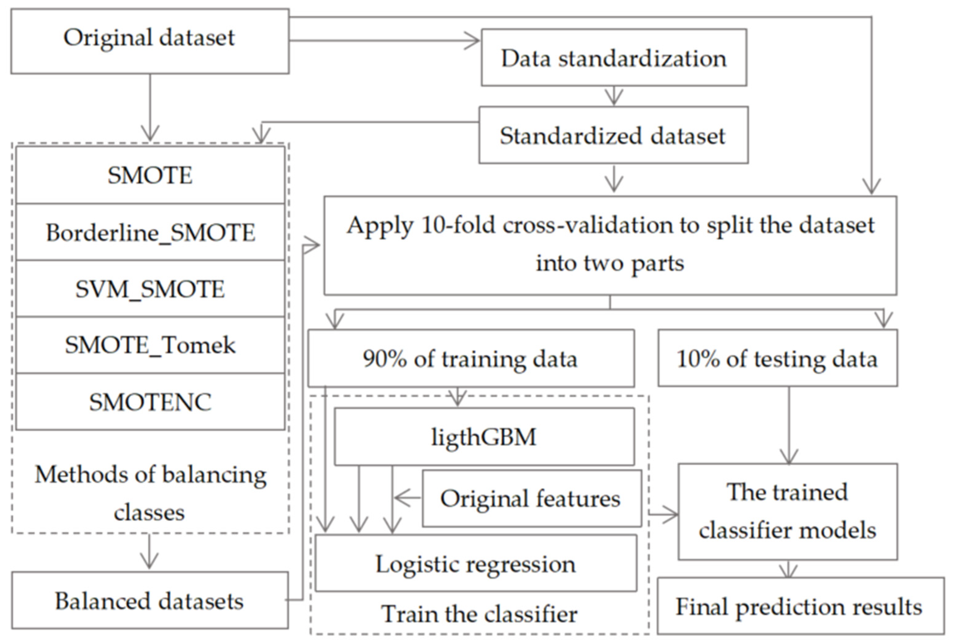
Figure 1.
The frame diagram of our proposed machine learning model.
Figure 1.
The frame diagram of our proposed machine learning model.
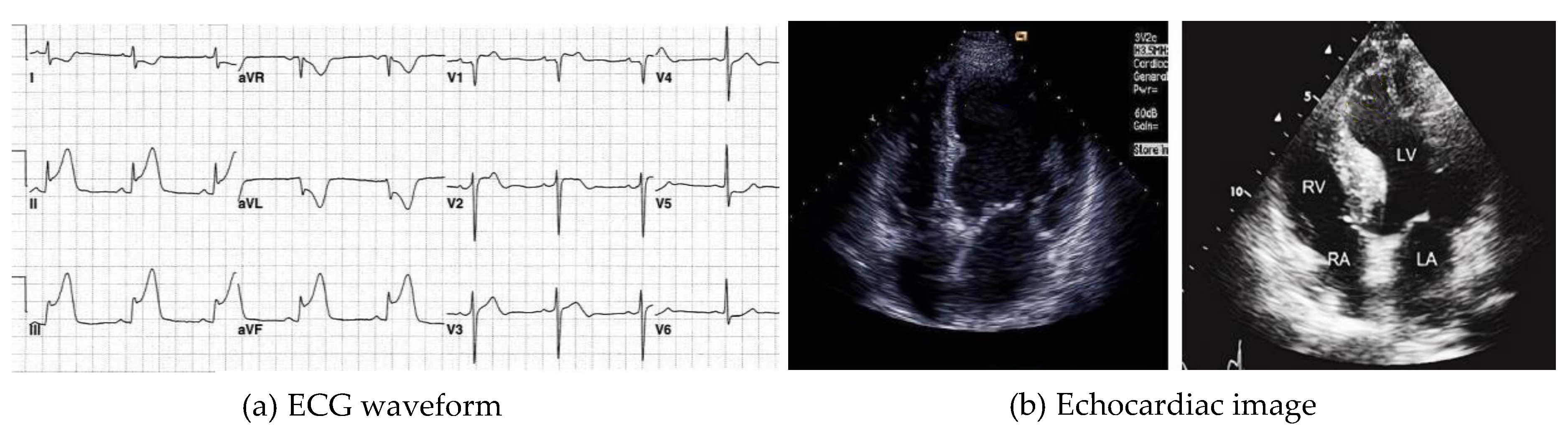
Figure 2.
An example of an ECG waveform and an echocardiac image (pictures from the Internet).
Figure 2.
An example of an ECG waveform and an echocardiac image (pictures from the Internet).
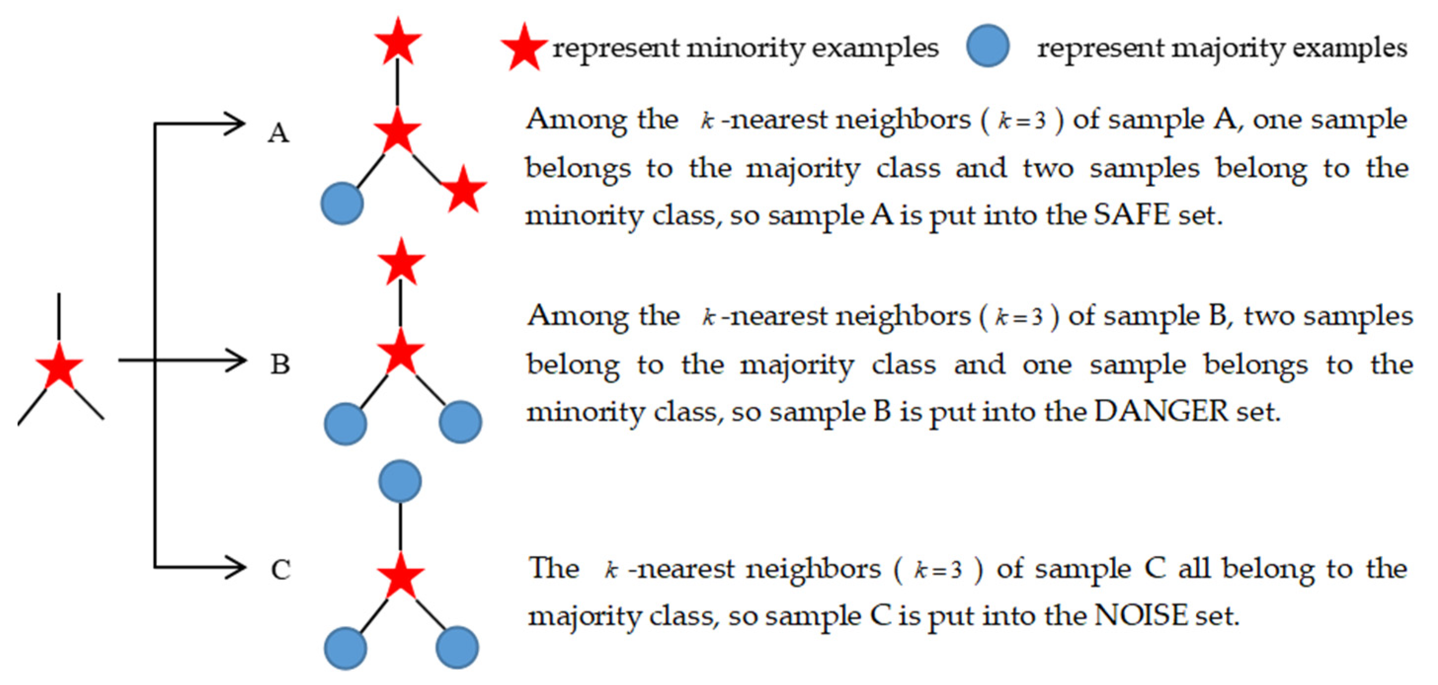
Figure 3.
Standard for Borderline_SMOTE algorithm to assign minority samples to SAFE set, DANGER set and NOISE set.
Figure 3.
Standard for Borderline_SMOTE algorithm to assign minority samples to SAFE set, DANGER set and NOISE set.
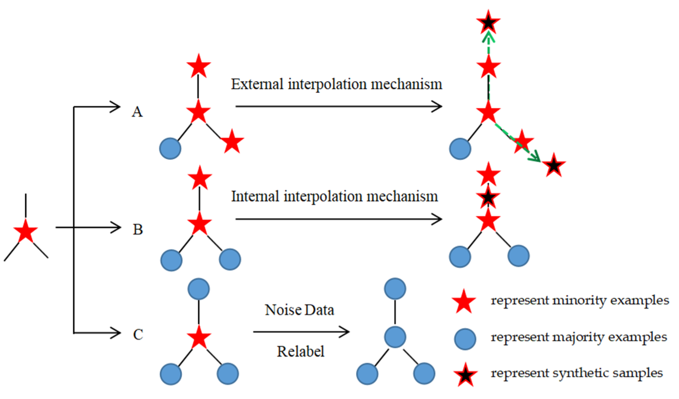
Figure 4.
The decision mechanism of SVM_SMOTE algorithm for synthesizing new minority samples. A, B and C are minority class support vector samples.
Figure 4.
The decision mechanism of SVM_SMOTE algorithm for synthesizing new minority samples. A, B and C are minority class support vector samples.
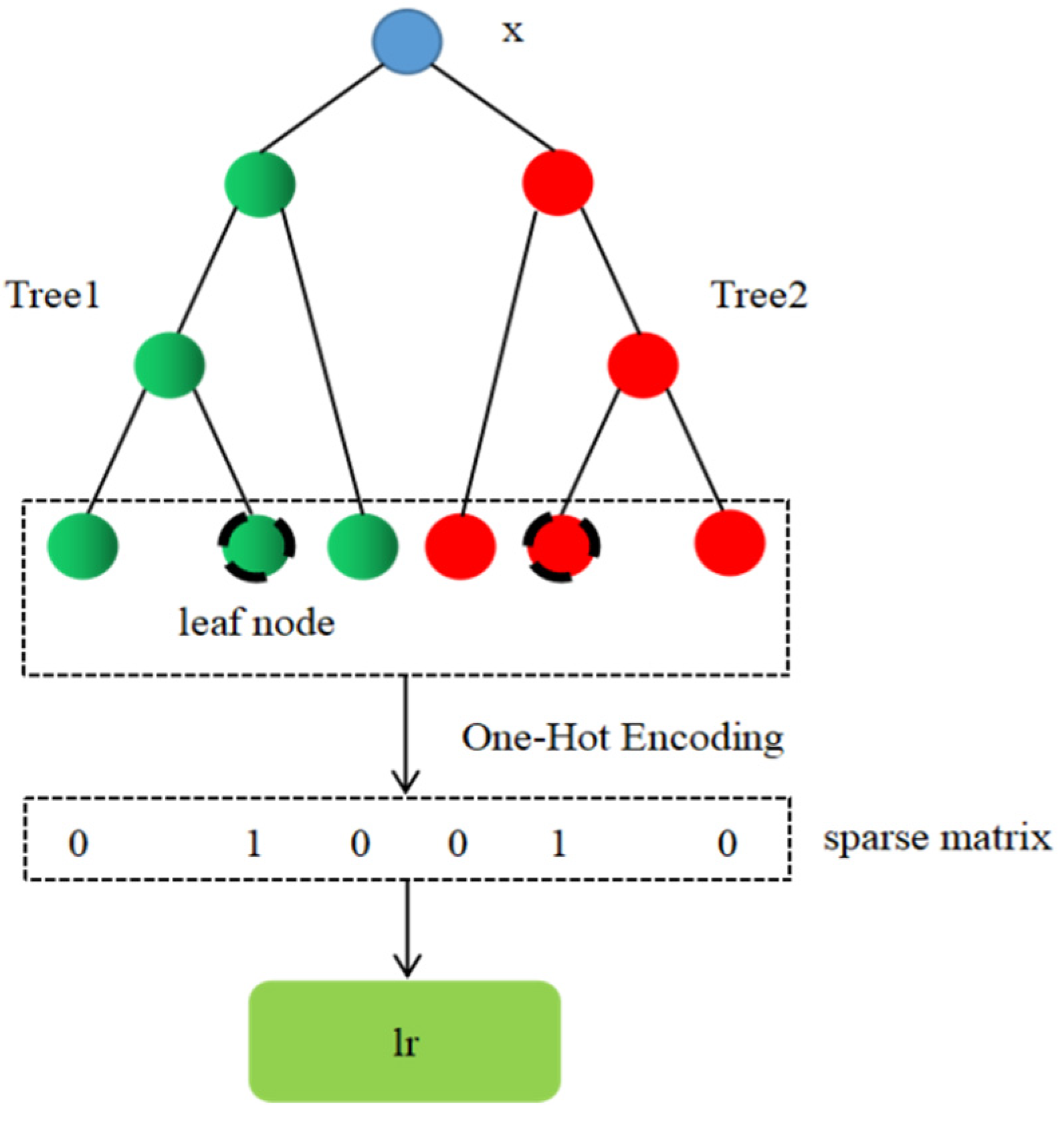
Figure 5.
The process of realizing automatic feature combination based on lightGBM model.
Figure 5.
The process of realizing automatic feature combination based on lightGBM model.
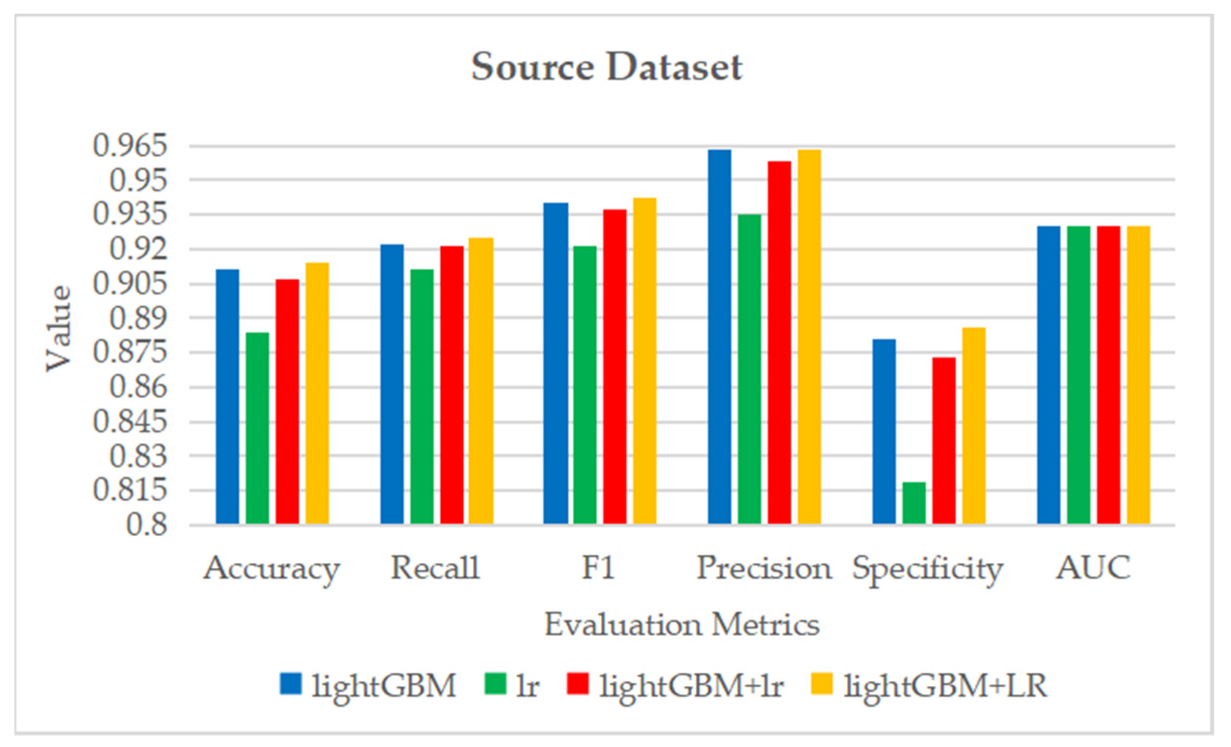
Figure 6.
The histogram of
Table 6.
Figure 6.
The histogram of
Table 6.
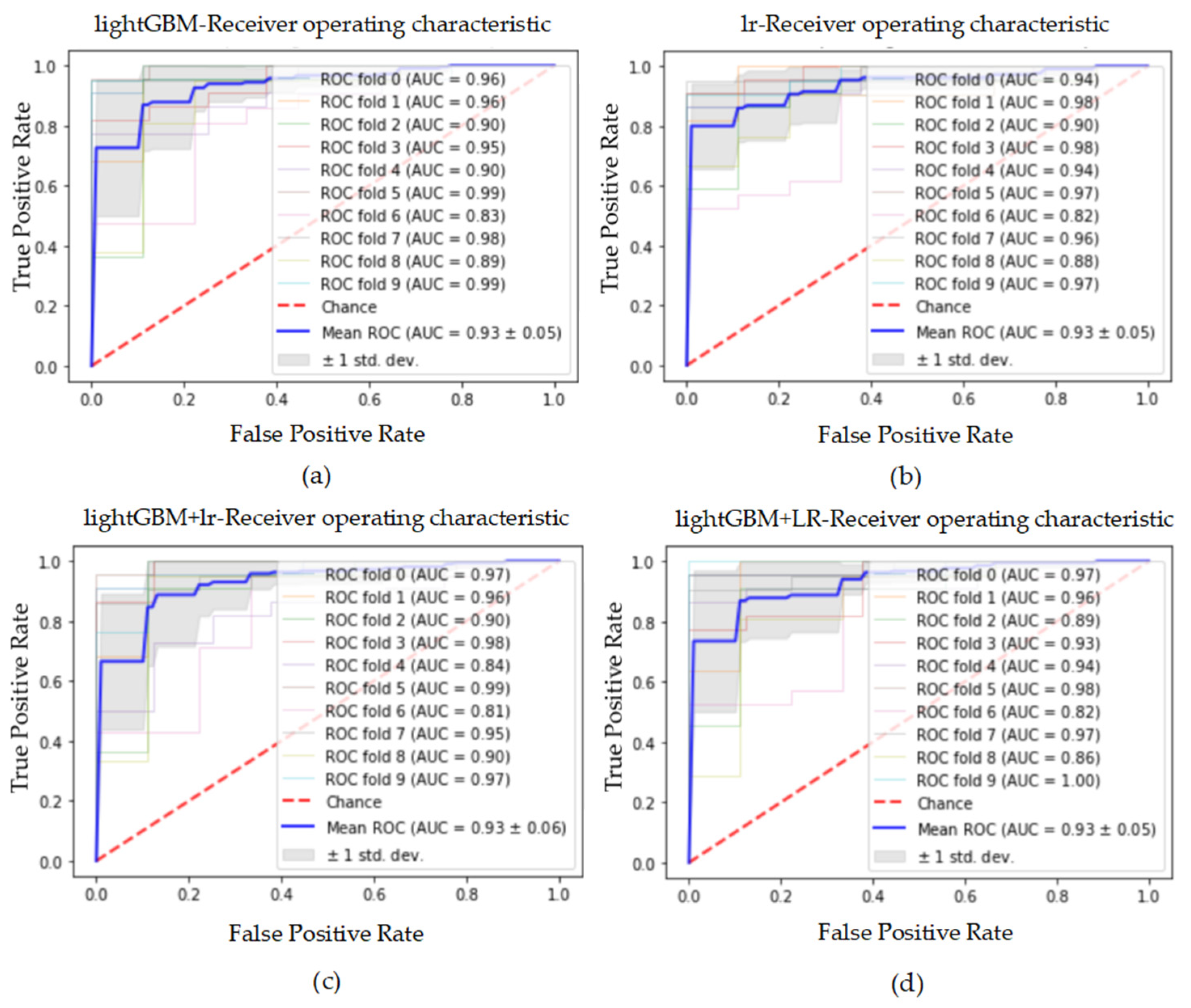
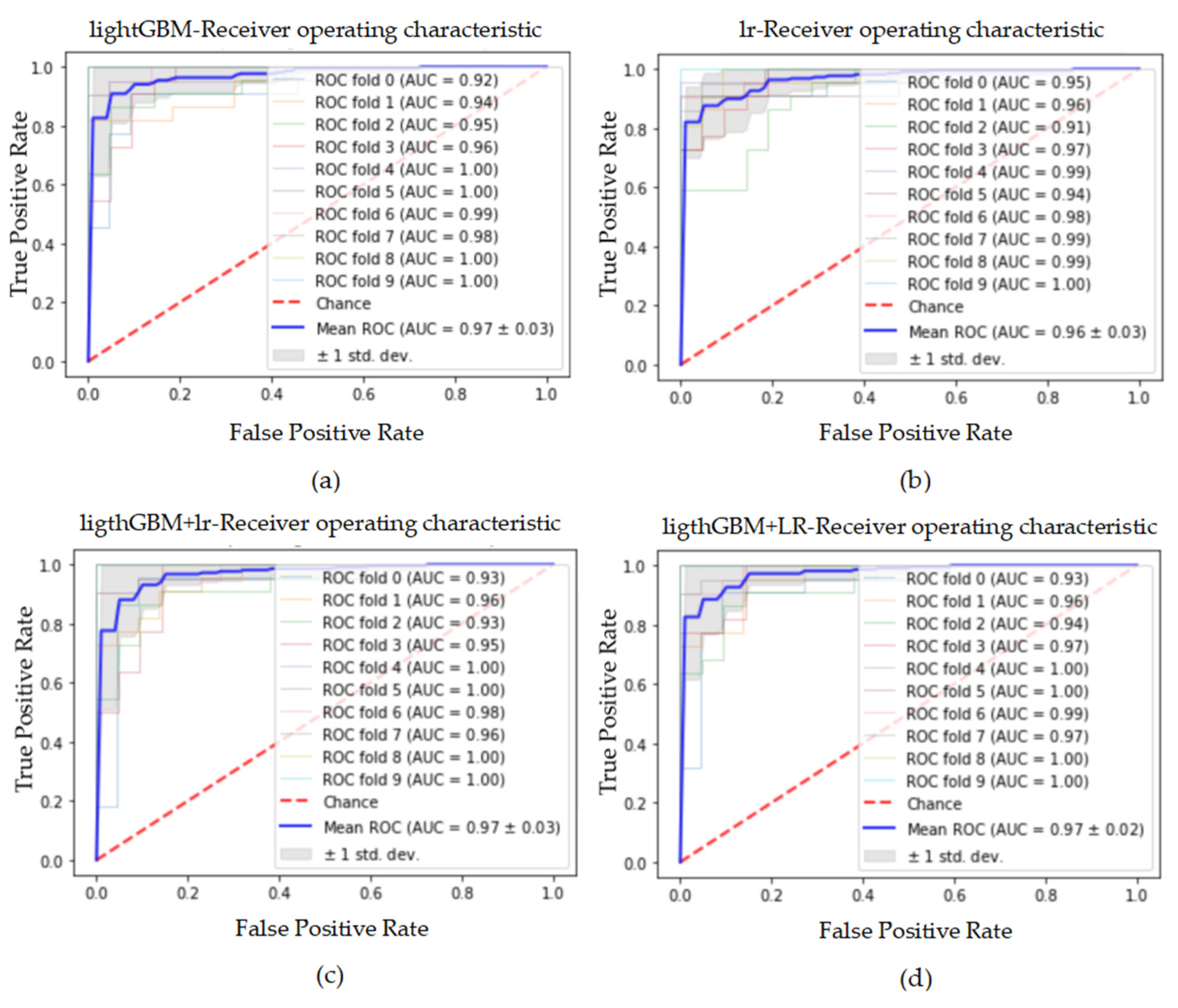
Figure 7.
The ROC curve and AUC value of each fold in the 10-fold cross-validation obtained by classification models on the original dataset. (a–d) are the ROC curves of lightGBM, lr, lightGBM + lr and lightGBM + LR classifiers, respectively.
Figure 7.
The ROC curve and AUC value of each fold in the 10-fold cross-validation obtained by classification models on the original dataset. (a–d) are the ROC curves of lightGBM, lr, lightGBM + lr and lightGBM + LR classifiers, respectively.
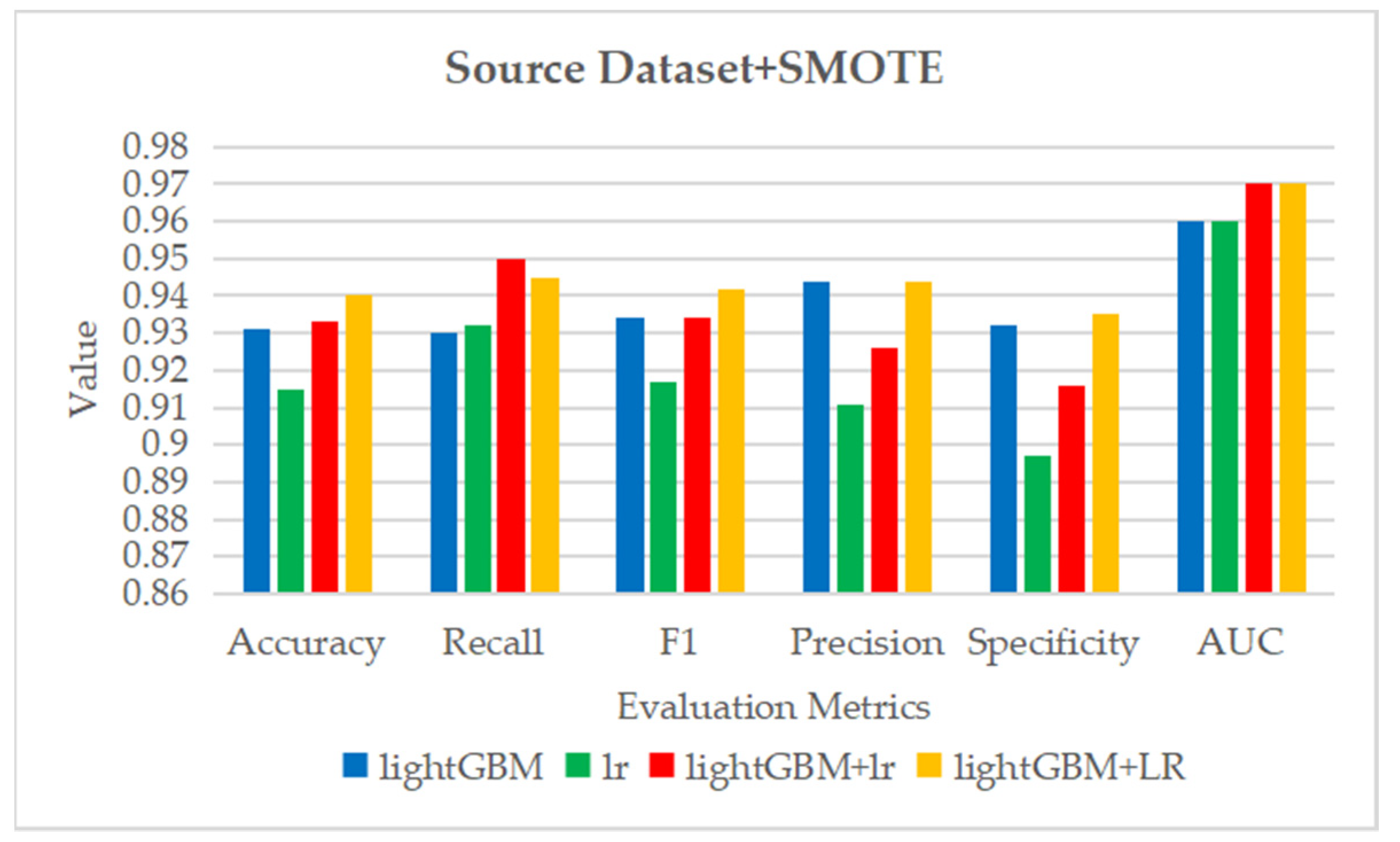
Figure 8.
The histogram of
Table 7.
Figure 8.
The histogram of
Table 7.
Figure 9.
The ROC curve and AUC value of each fold in the 10-fold cross-validation obtained by classification models on the dataset processed by SMOTE. (a–d) are the ROC curves of lightGBM, lr, lightGBM + lr and lightGBM + LR classifiers, respectively.
Figure 9.
The ROC curve and AUC value of each fold in the 10-fold cross-validation obtained by classification models on the dataset processed by SMOTE. (a–d) are the ROC curves of lightGBM, lr, lightGBM + lr and lightGBM + LR classifiers, respectively.
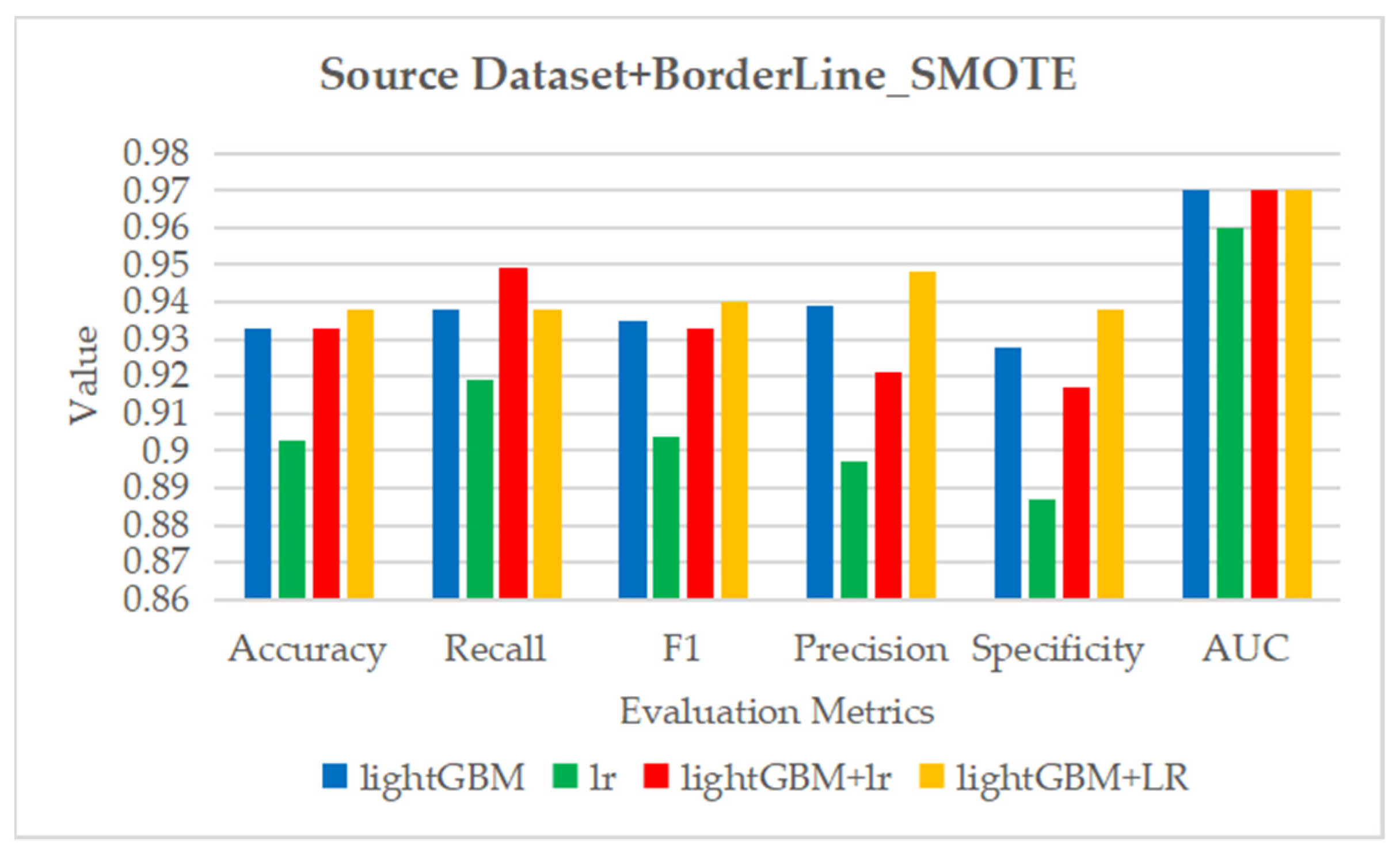
Figure 10.
The histogram of
Table 8.
Figure 10.
The histogram of
Table 8.
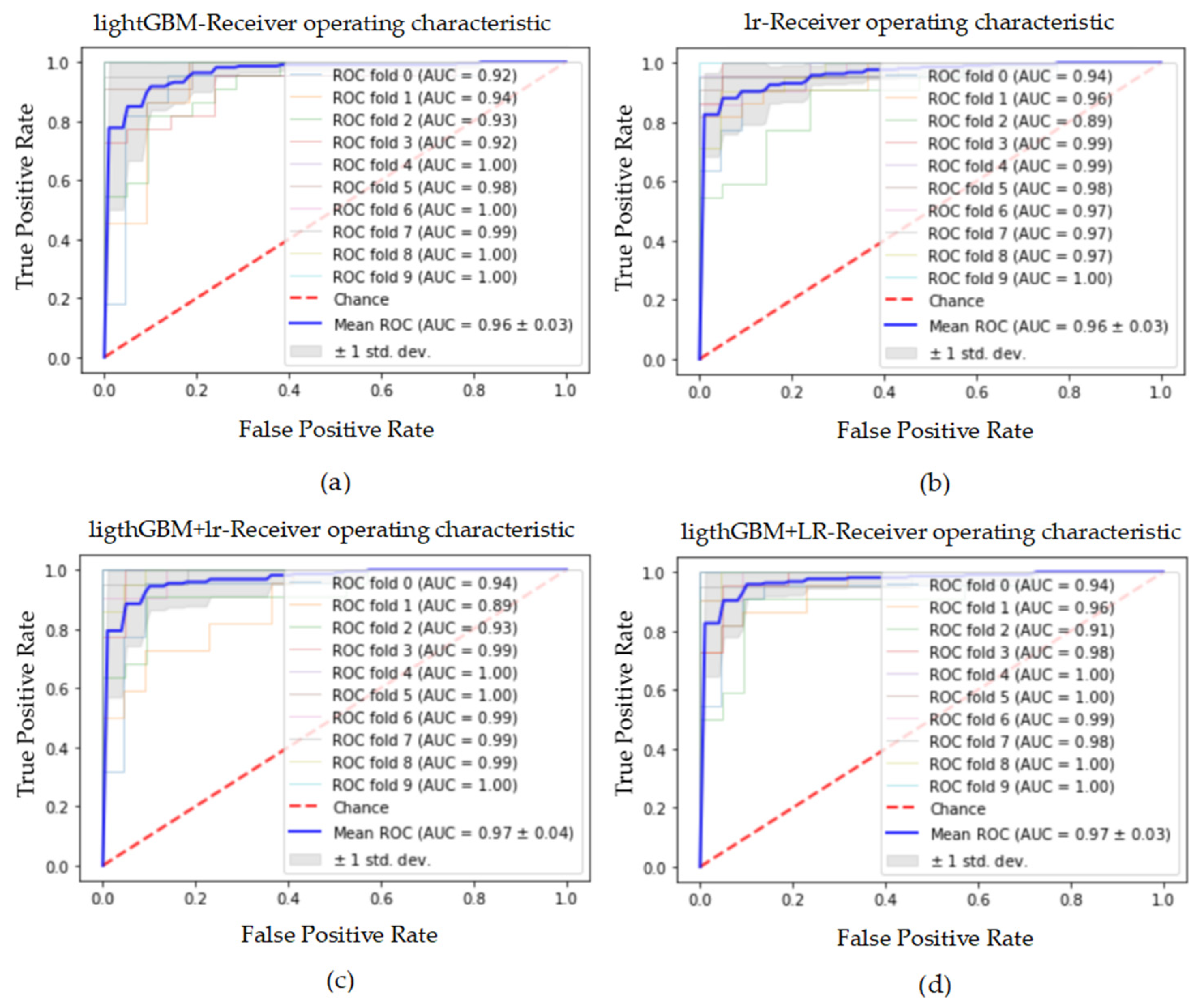
Figure 11.
The ROC curve and AUC value of each fold in the 10-fold cross-validation obtained by classification models on the dataset processed by Borderline_SMOTE. (a–d) are the ROC curves of lightGBM, lr, lightGBM + lr and lightGBM + LR classifiers, respectively.
Figure 11.
The ROC curve and AUC value of each fold in the 10-fold cross-validation obtained by classification models on the dataset processed by Borderline_SMOTE. (a–d) are the ROC curves of lightGBM, lr, lightGBM + lr and lightGBM + LR classifiers, respectively.
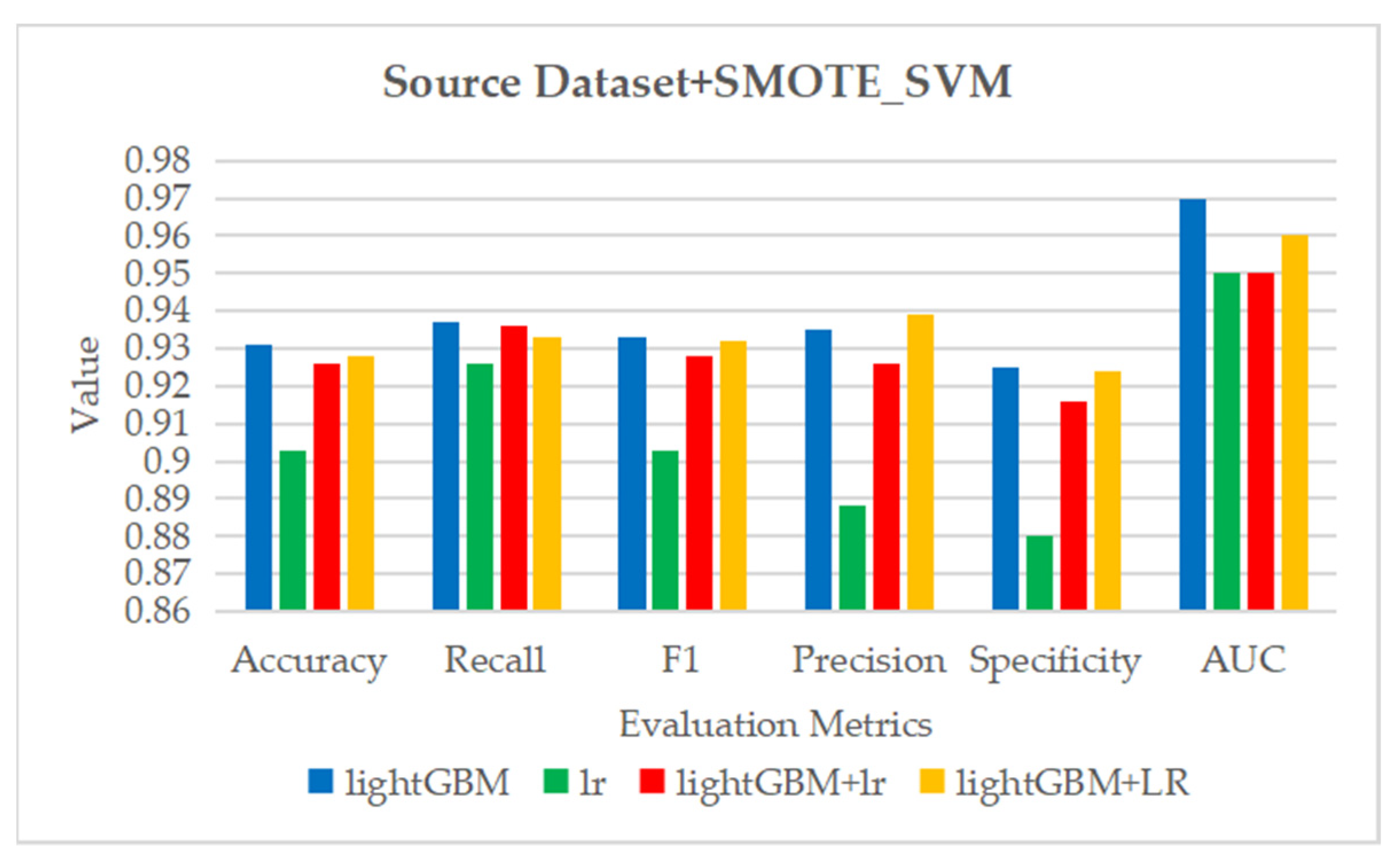
Figure 12.
The histogram of
Table 9.
Figure 12.
The histogram of
Table 9.
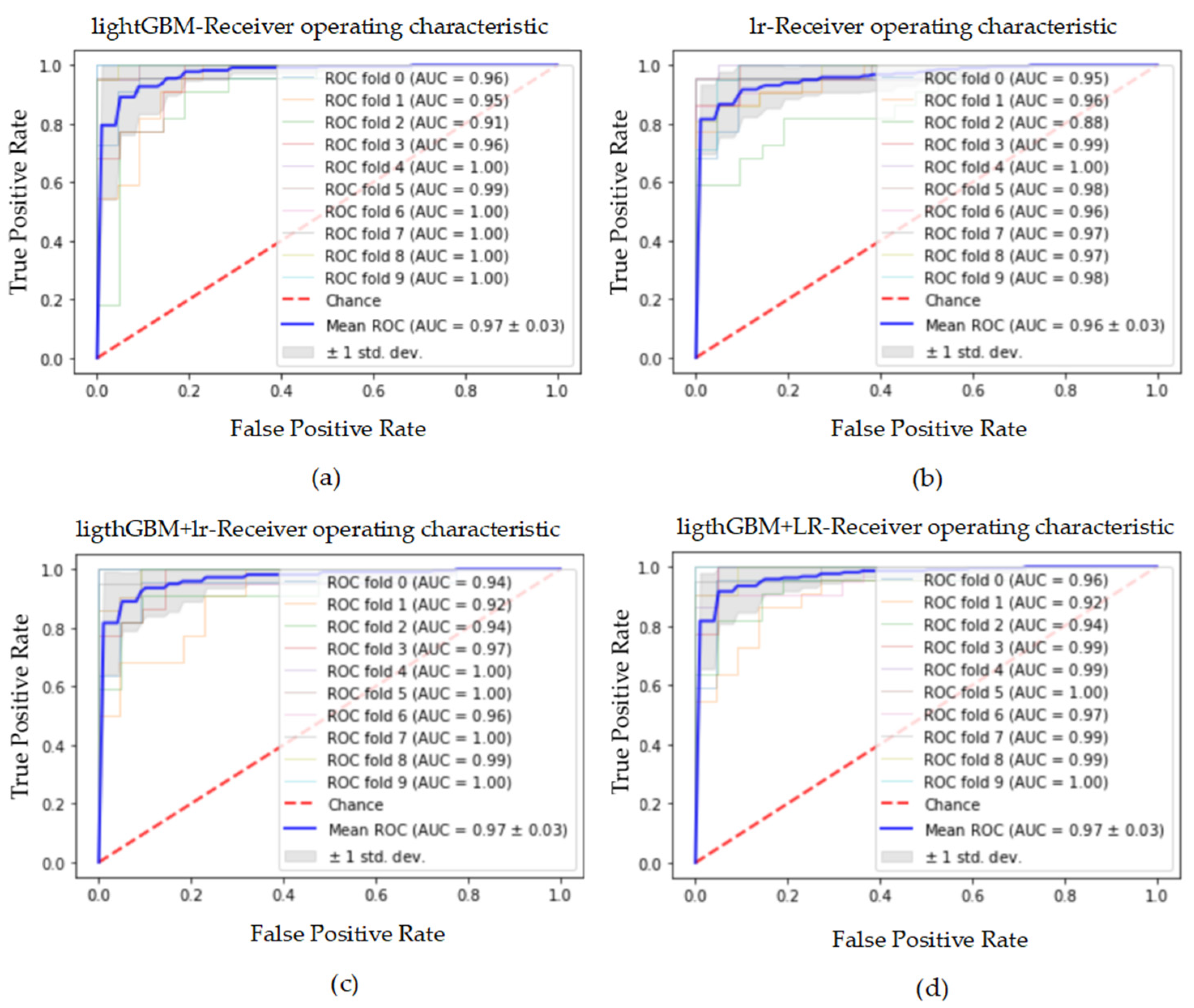
Figure 13.
The ROC curve and AUC value of each fold in the 10-fold cross-validation obtained by classification models on the dataset processed by SMOTE_SVM. (a–d) are the ROC curves of lightGBM, lr, lightGBM + lr and lightGBM + LR classifiers, respectively.
Figure 13.
The ROC curve and AUC value of each fold in the 10-fold cross-validation obtained by classification models on the dataset processed by SMOTE_SVM. (a–d) are the ROC curves of lightGBM, lr, lightGBM + lr and lightGBM + LR classifiers, respectively.
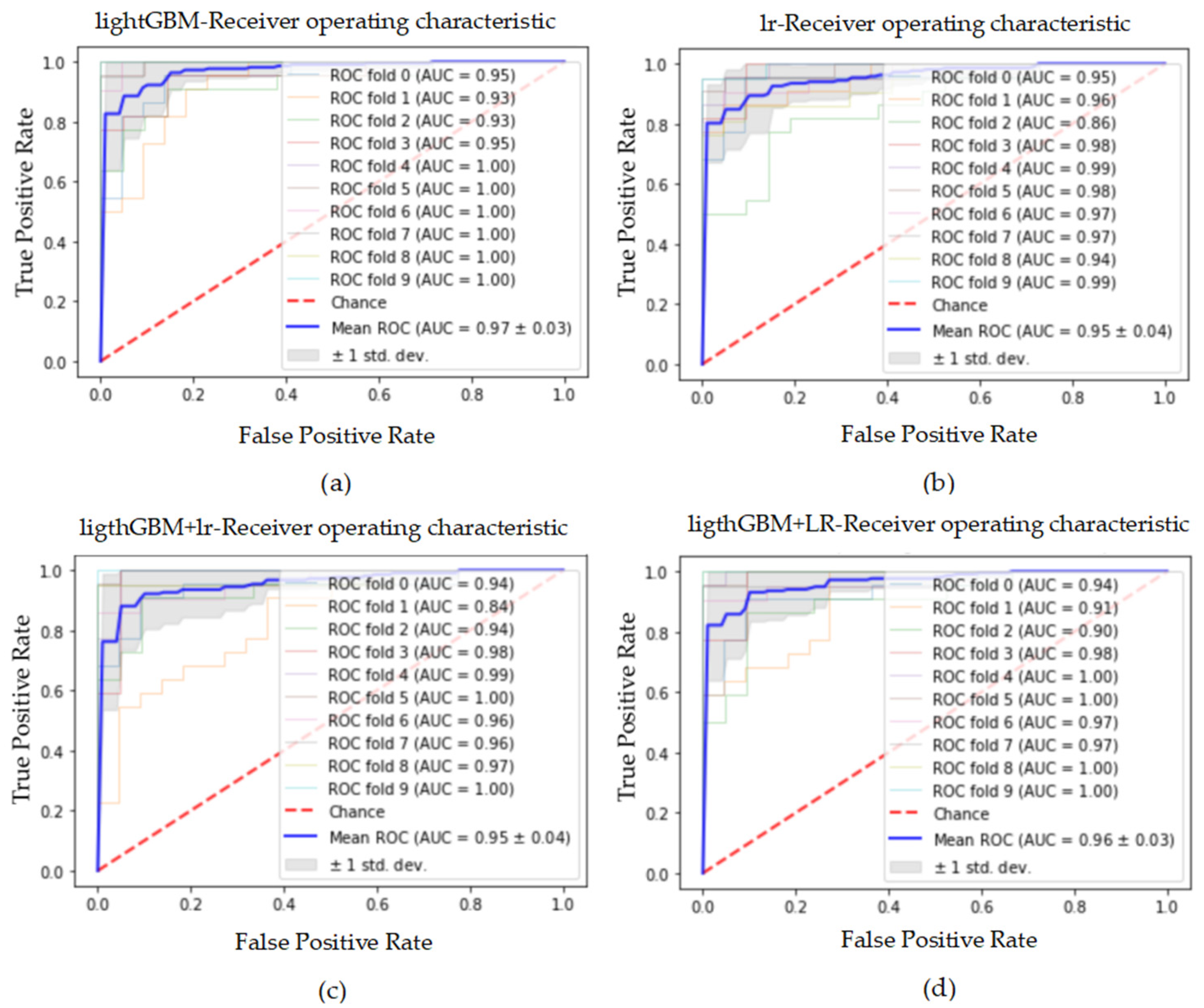
Figure 15.
The ROC curve and AUC value of each fold in the 10-fold cross-validation obtained by classification models on the dataset processed by SMOTE_Tomek. (a–d) are the ROC curves of lightGBM, lr, lightGBM + lr and lightGBM + LR classifiers, respectively.
Figure 15.
The ROC curve and AUC value of each fold in the 10-fold cross-validation obtained by classification models on the dataset processed by SMOTE_Tomek. (a–d) are the ROC curves of lightGBM, lr, lightGBM + lr and lightGBM + LR classifiers, respectively.
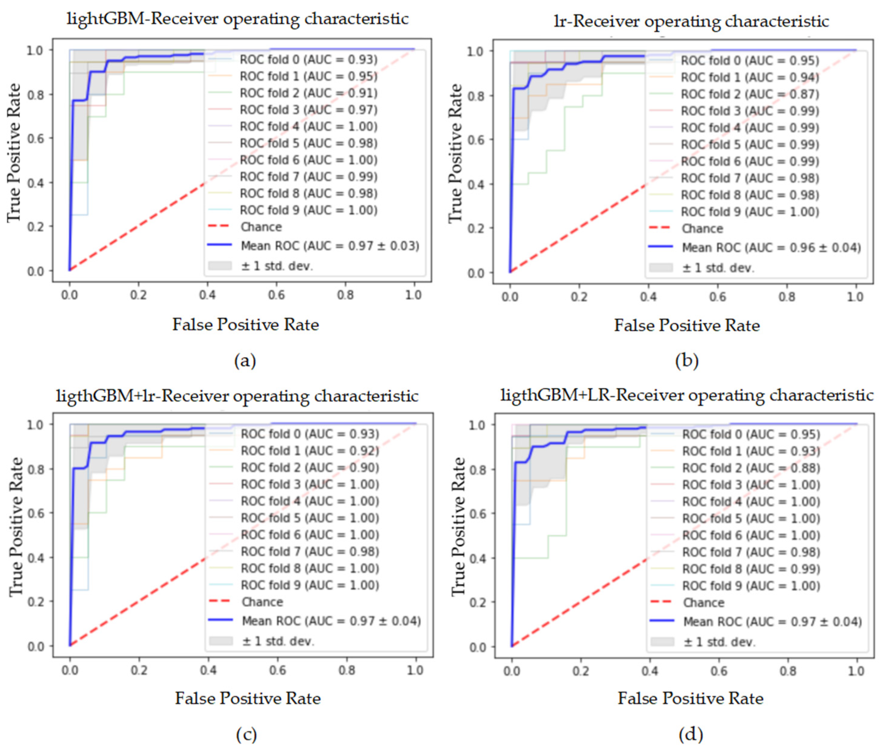
Figure 17.
The ROC curve and AUC value of each fold in the 10-fold cross-validation obtained by classification models on the dataset processed by SMOTENC. (a–d) are the ROC curves of lightGBM, lr, lightGBM + lr and lightGBM + LR classifiers, respectively.
Figure 17.
The ROC curve and AUC value of each fold in the 10-fold cross-validation obtained by classification models on the dataset processed by SMOTENC. (a–d) are the ROC curves of lightGBM, lr, lightGBM + lr and lightGBM + LR classifiers, respectively.
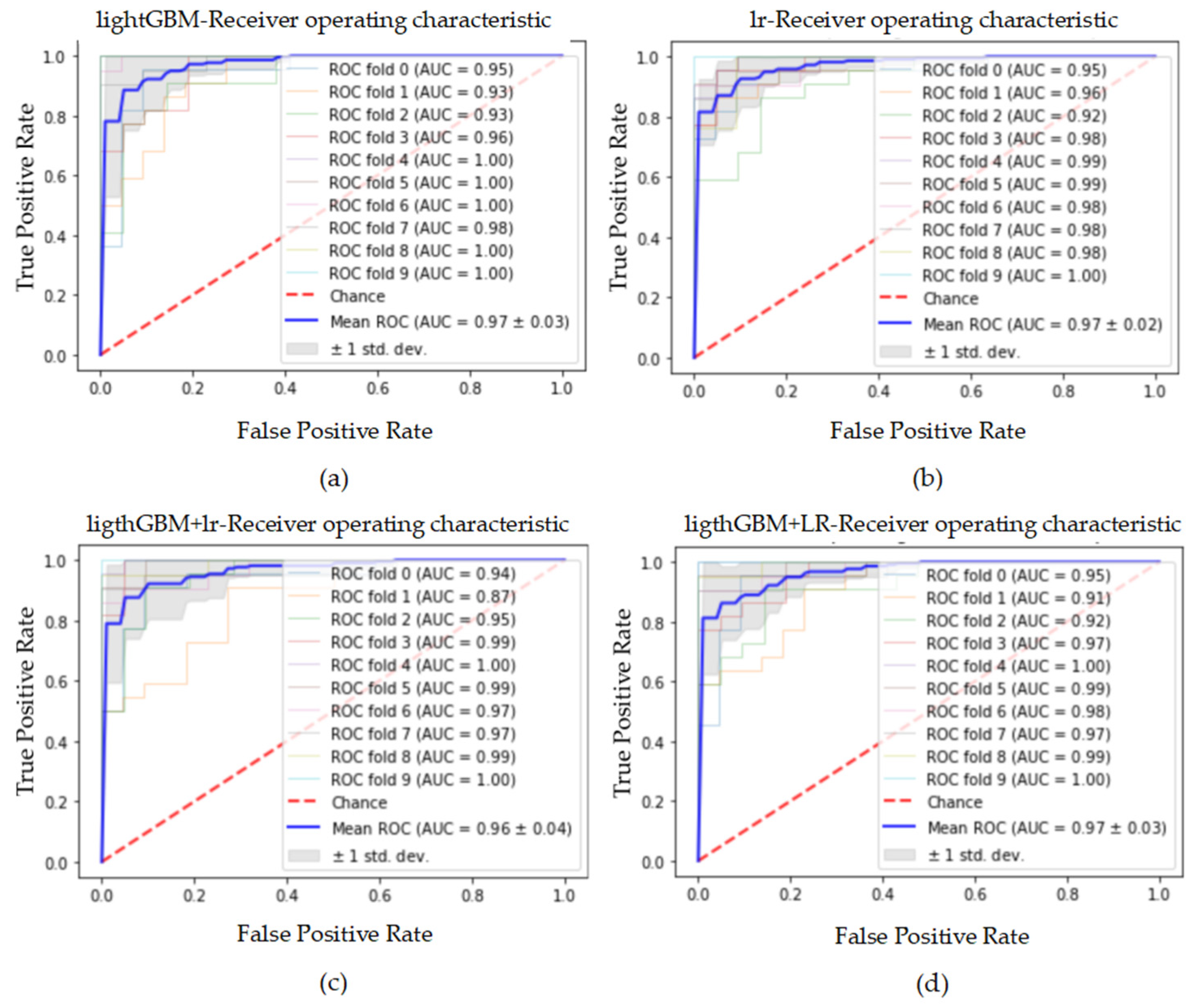
Figure 19.
The ROC curve and AUC value of each fold in the 10-fold cross-validation obtained by classification models on the dataset processed by data standardization. (a–d) are the ROC curves of lightGBM, lr, lightGBM + lr and lightGBM + LR classifiers, respectively.
Figure 19.
The ROC curve and AUC value of each fold in the 10-fold cross-validation obtained by classification models on the dataset processed by data standardization. (a–d) are the ROC curves of lightGBM, lr, lightGBM + lr and lightGBM + LR classifiers, respectively.
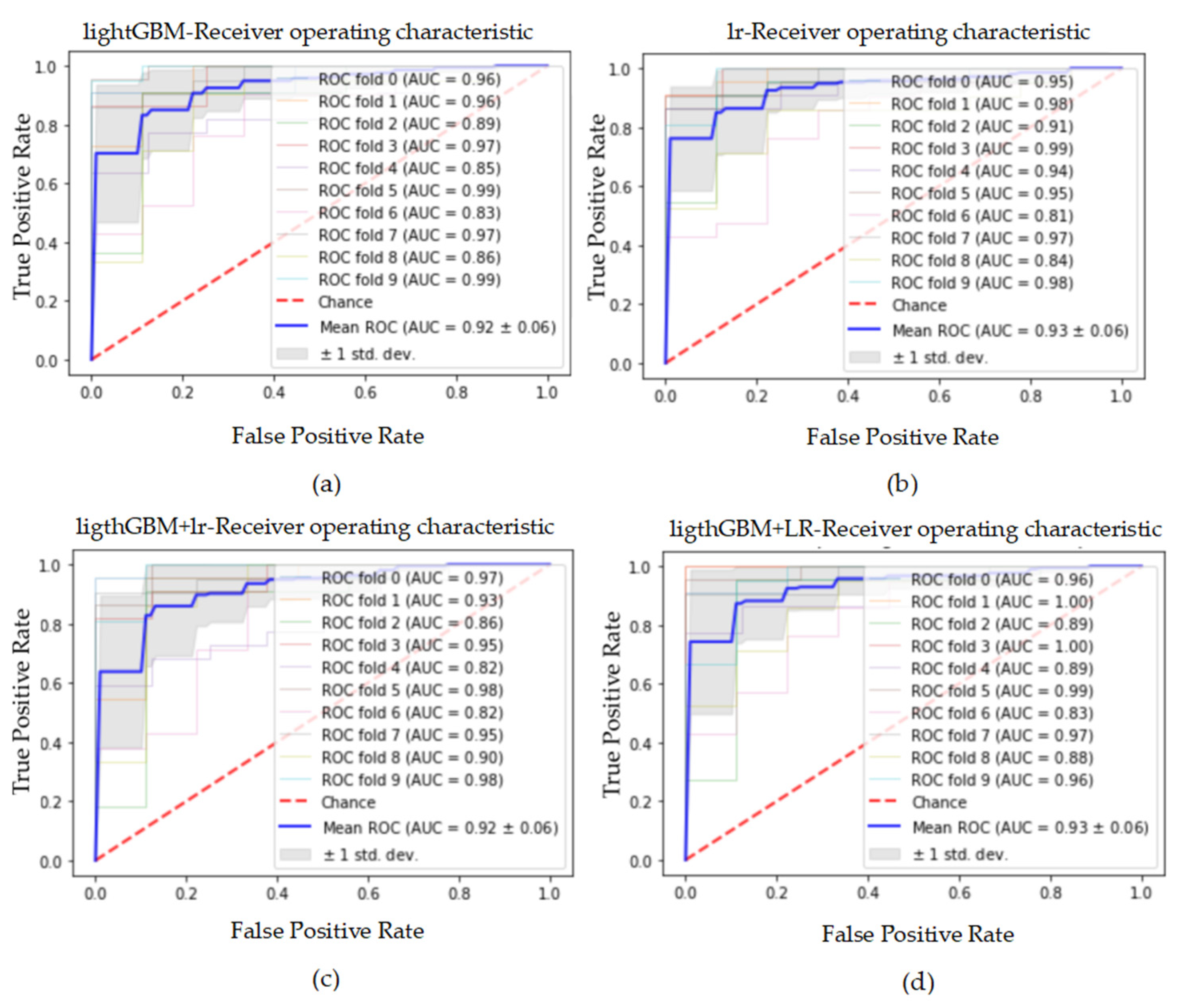
Figure 21.
The ROC curve and AUC value of each fold in the 10-fold cross-validation obtained by classification models on the dataset processed by data standardization and SMOTE. (a–d) are the ROC curves of lightGBM, lr, lightGBM + lr and lightGBM + LR classifiers, respectively.
Figure 21.
The ROC curve and AUC value of each fold in the 10-fold cross-validation obtained by classification models on the dataset processed by data standardization and SMOTE. (a–d) are the ROC curves of lightGBM, lr, lightGBM + lr and lightGBM + LR classifiers, respectively.
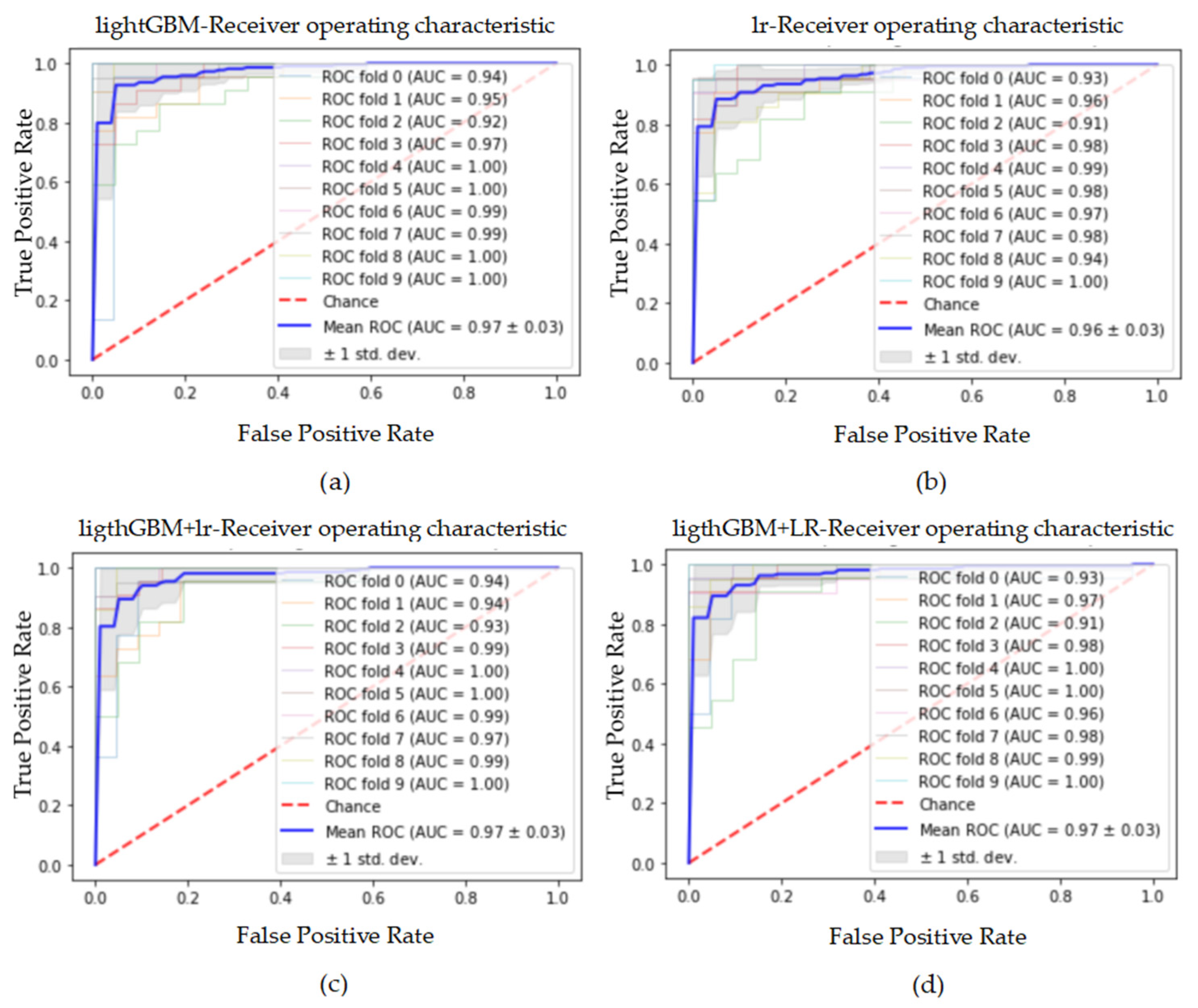
Figure 23.
The ROC curve and AUC value of each fold in the 10-fold cross-validation obtained by classification models on the dataset processed by data standardization and Borderline_SMOTE. (a–d) are the ROC curves of lightGBM, lr, lightGBM + lr and lightGBM + LR classifiers, respectively.
Figure 23.
The ROC curve and AUC value of each fold in the 10-fold cross-validation obtained by classification models on the dataset processed by data standardization and Borderline_SMOTE. (a–d) are the ROC curves of lightGBM, lr, lightGBM + lr and lightGBM + LR classifiers, respectively.
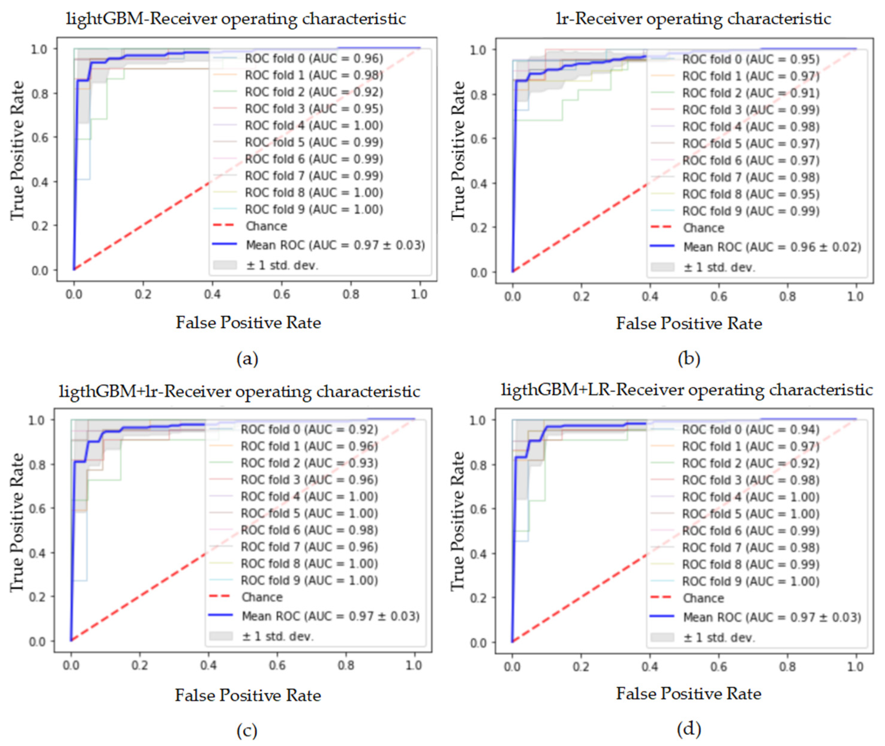
Figure 25.
The ROC curve and AUC value of each fold in the 10-fold cross-validation obtained by classification models on the dataset processed by data standardization and SMOTE_SVM. (a–d) are the ROC curves of lightGBM, lr, lightGBM + lr and lightGBM + LR classifiers, respectively.
Figure 25.
The ROC curve and AUC value of each fold in the 10-fold cross-validation obtained by classification models on the dataset processed by data standardization and SMOTE_SVM. (a–d) are the ROC curves of lightGBM, lr, lightGBM + lr and lightGBM + LR classifiers, respectively.
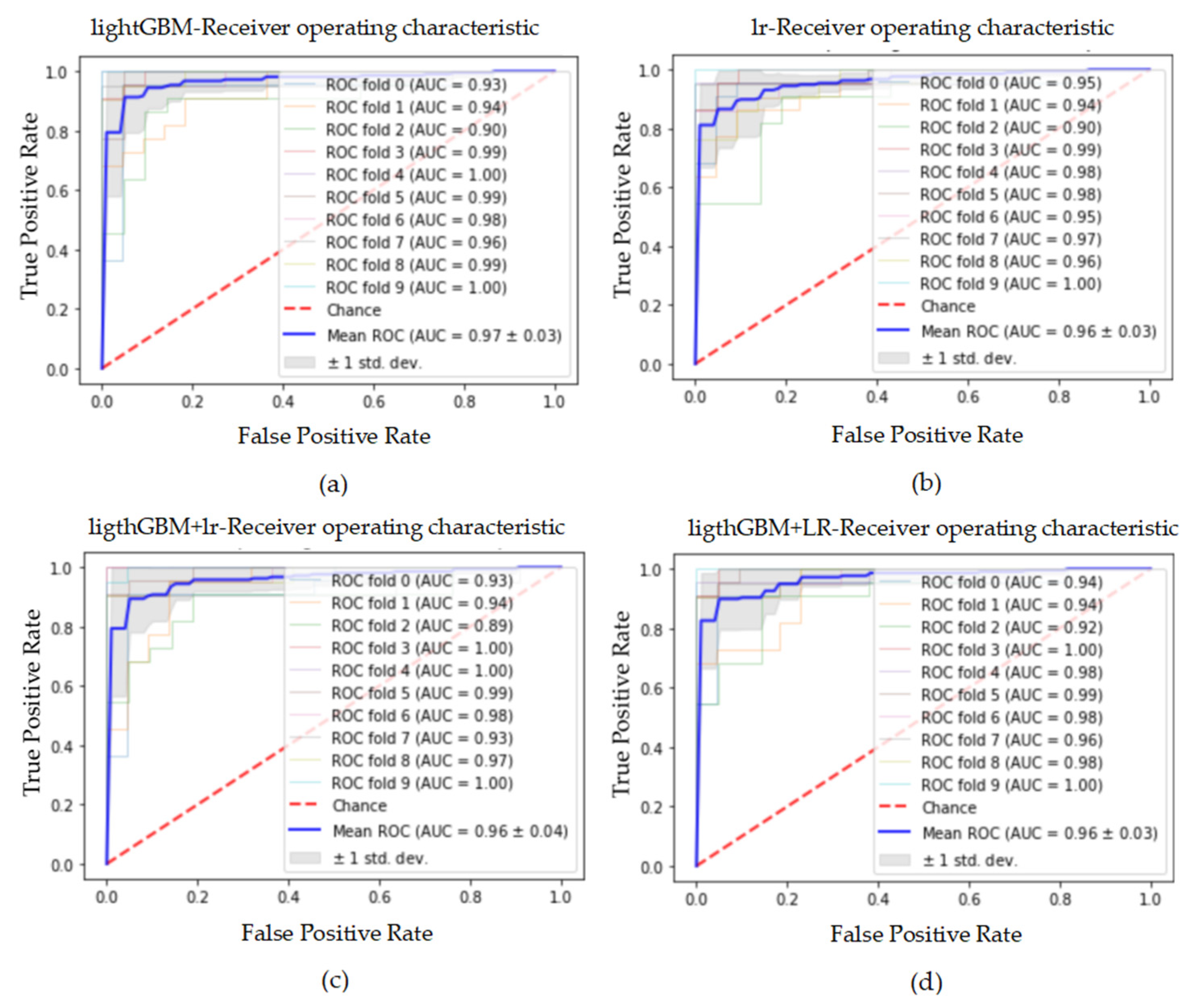
Figure 27.
The ROC curve and AUC value of each fold in the 10-fold cross-validation obtained by classification models on the dataset processed by data standardization and SMOTE_Tomek. (a–d) are the ROC curves of lightGBM, lr, lightGBM + lr and lightGBM + LR classifiers, respectively.
Figure 27.
The ROC curve and AUC value of each fold in the 10-fold cross-validation obtained by classification models on the dataset processed by data standardization and SMOTE_Tomek. (a–d) are the ROC curves of lightGBM, lr, lightGBM + lr and lightGBM + LR classifiers, respectively.
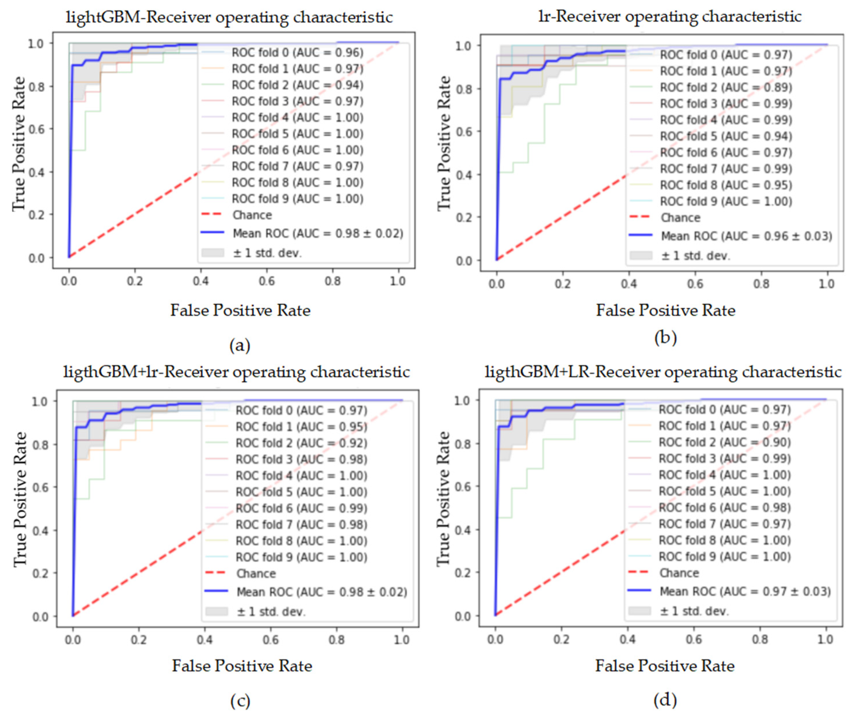
Figure 29.
The ROC curve and AUC value of each fold in the 10-fold cross-validation obtained by classification models on the dataset processed by data standardization and SMOTENC. (a–d) are the ROC curves of lightGBM, lr, lightGBM + lr and lightGBM + LR classifiers, respectively.
Figure 29.
The ROC curve and AUC value of each fold in the 10-fold cross-validation obtained by classification models on the dataset processed by data standardization and SMOTENC. (a–d) are the ROC curves of lightGBM, lr, lightGBM + lr and lightGBM + LR classifiers, respectively.
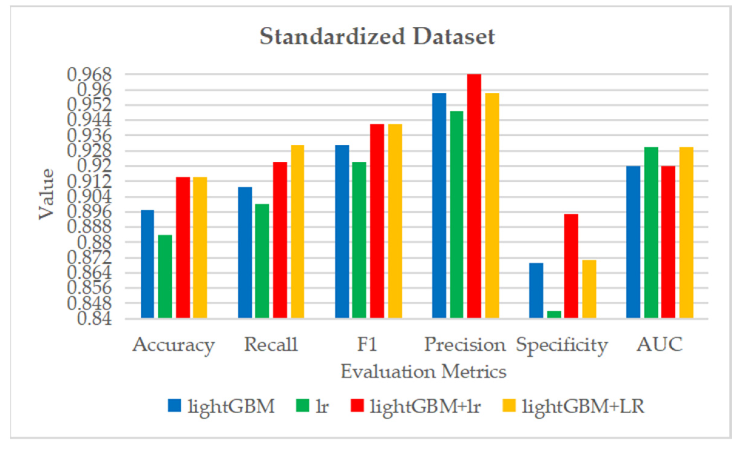
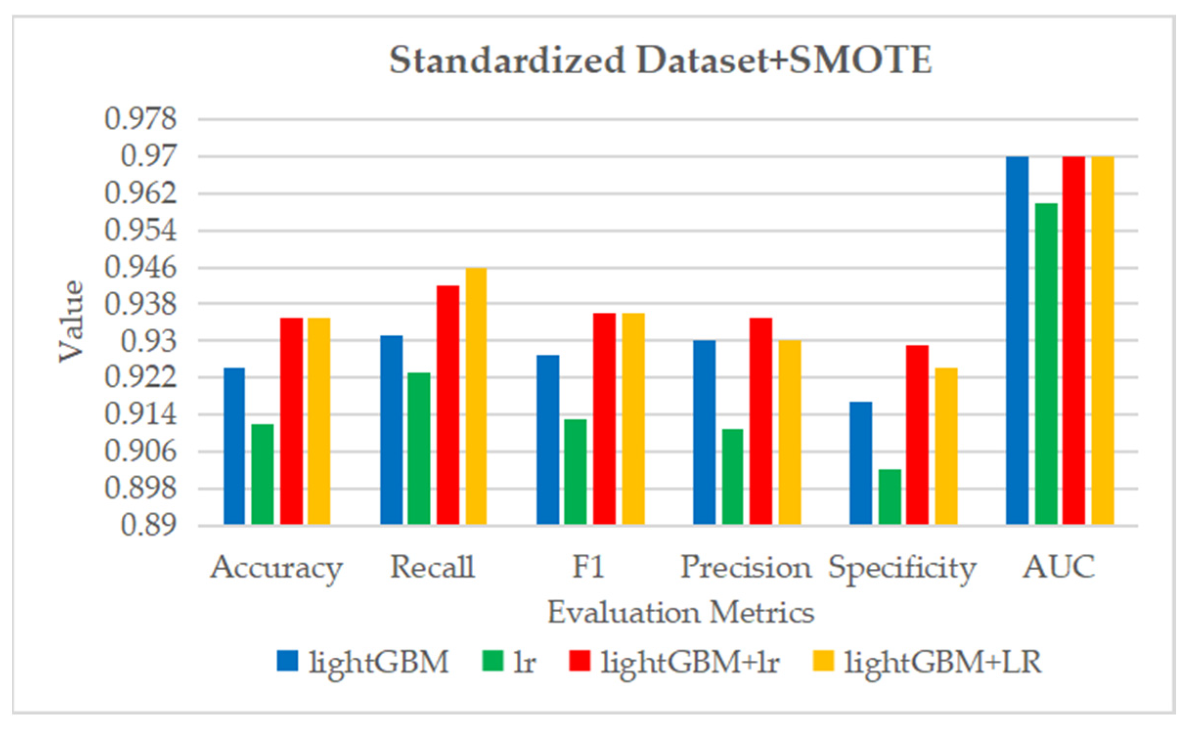
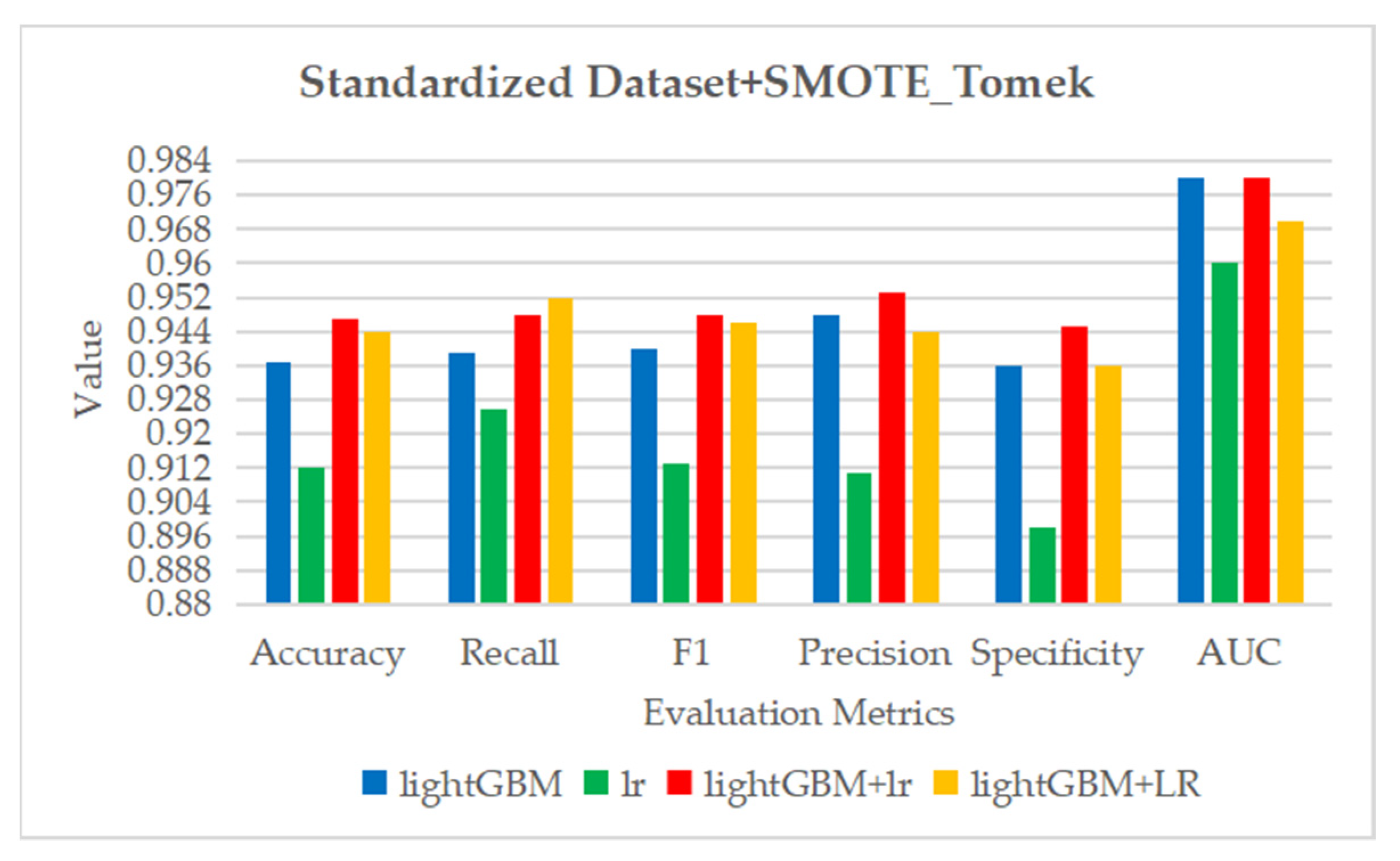
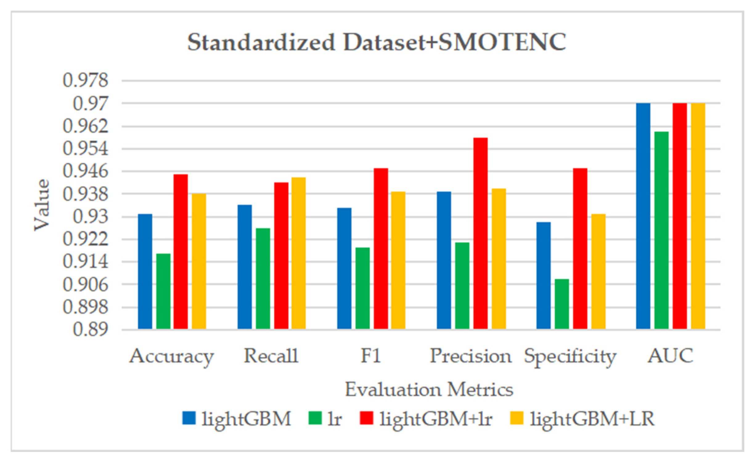
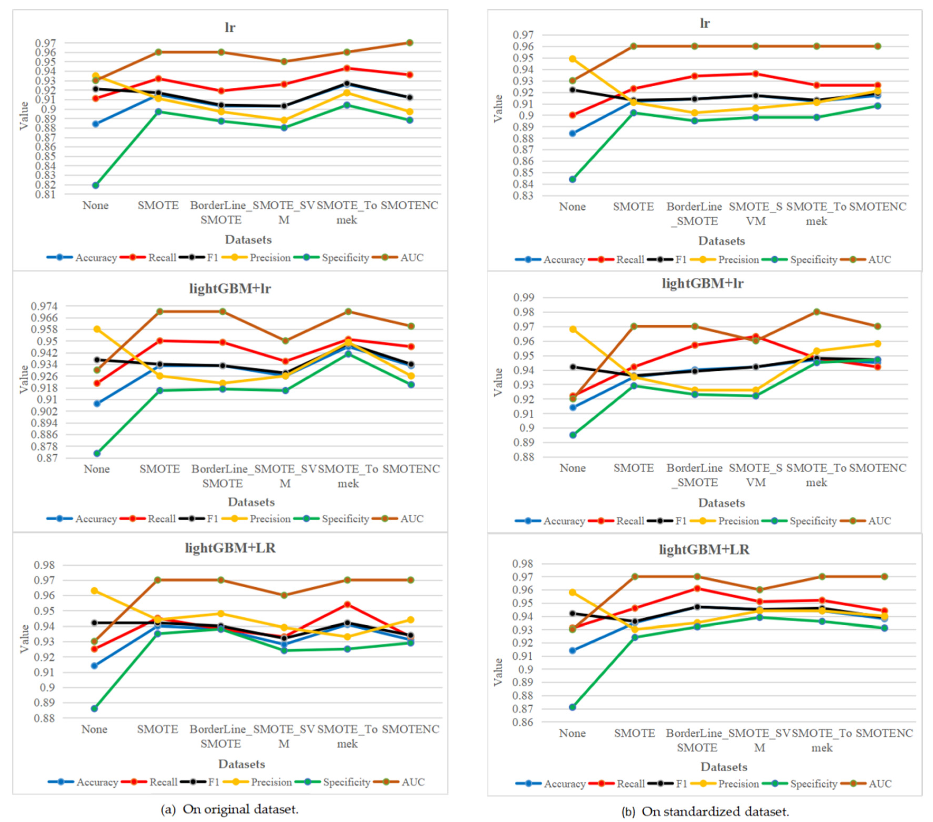
Figure 30.
The trend charts of the performance evaluation indexes with class balancing methods on original dataset and standardized dataset.
Figure 30.
The trend charts of the performance evaluation indexes with class balancing methods on original dataset and standardized dataset.
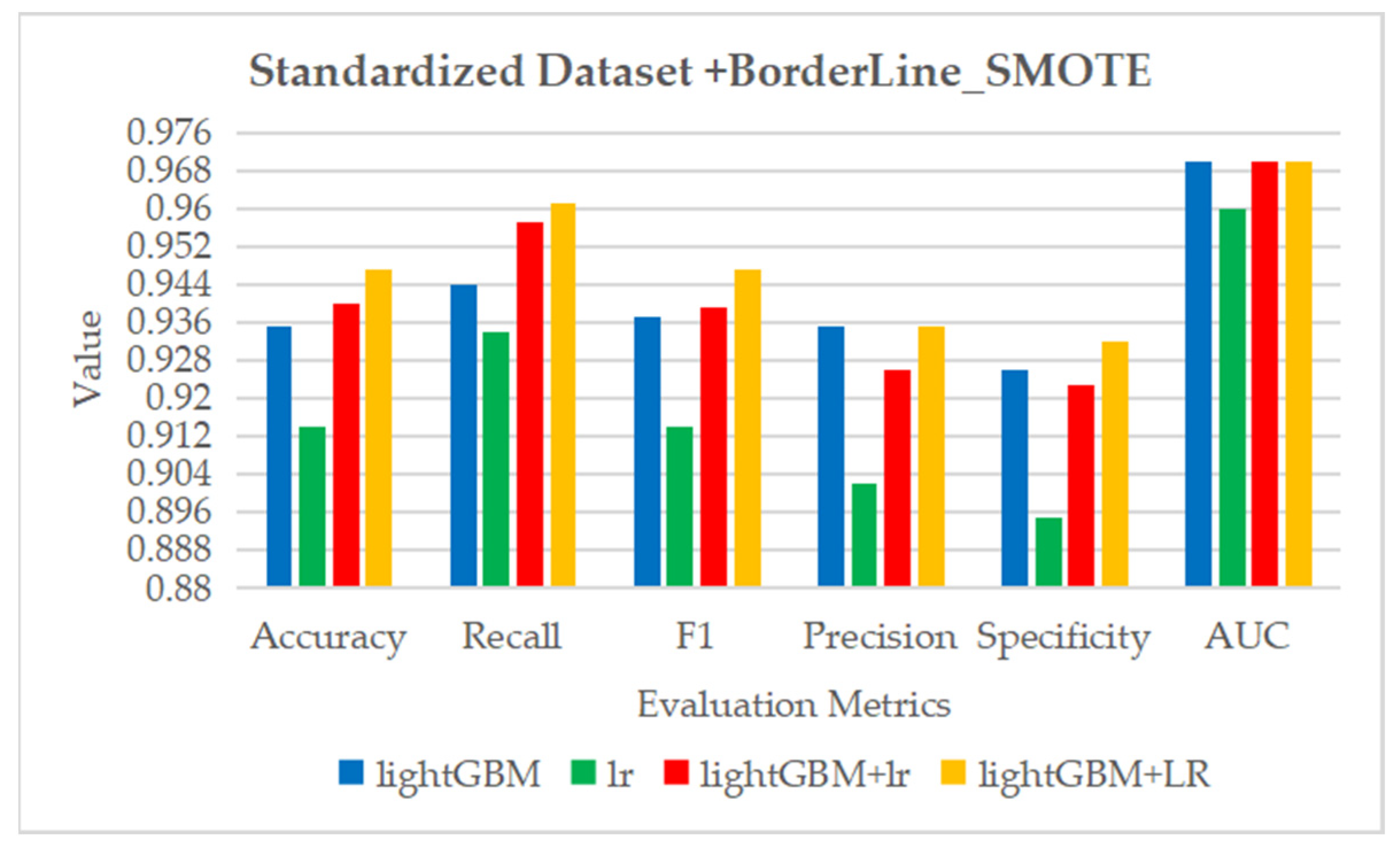
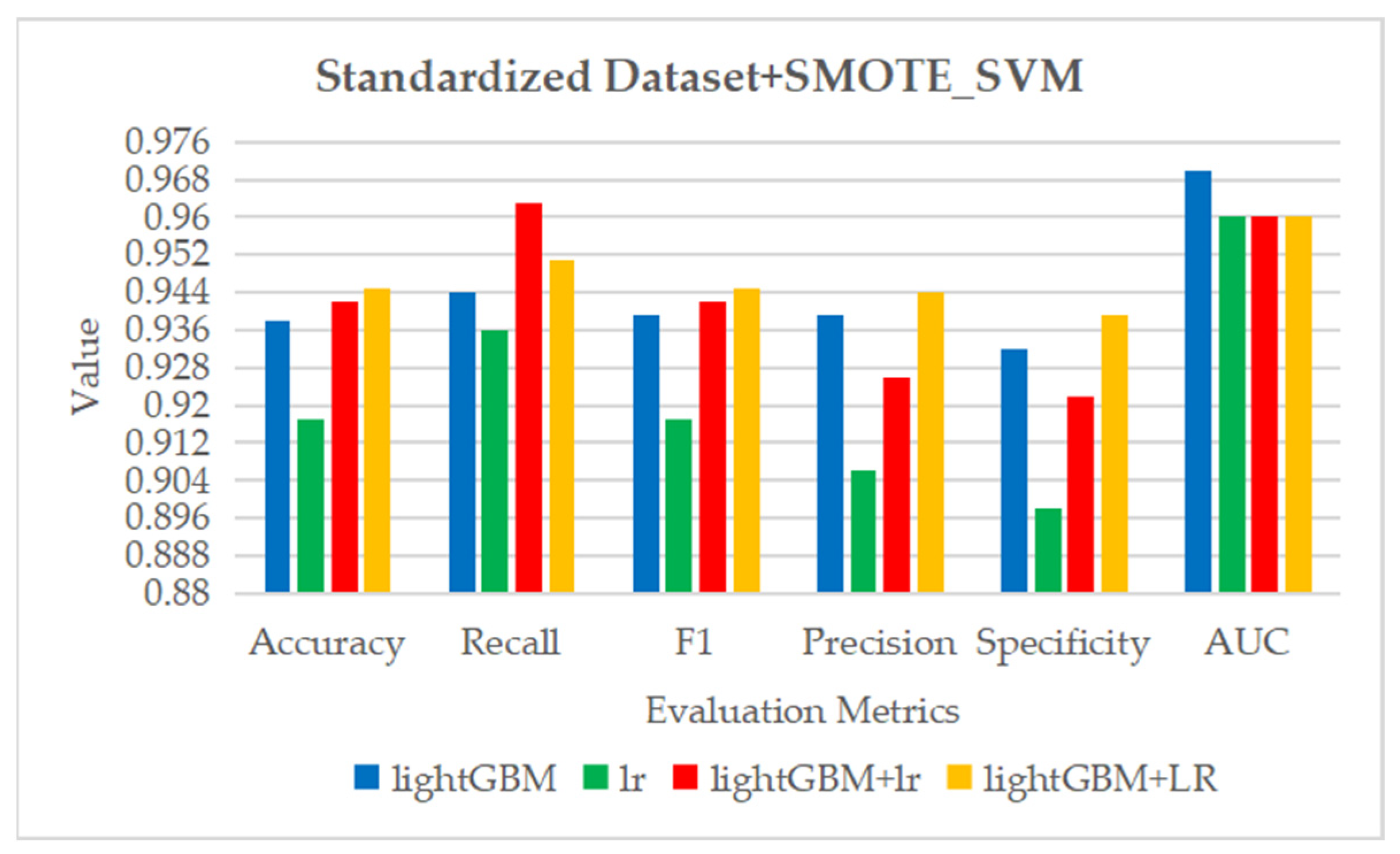
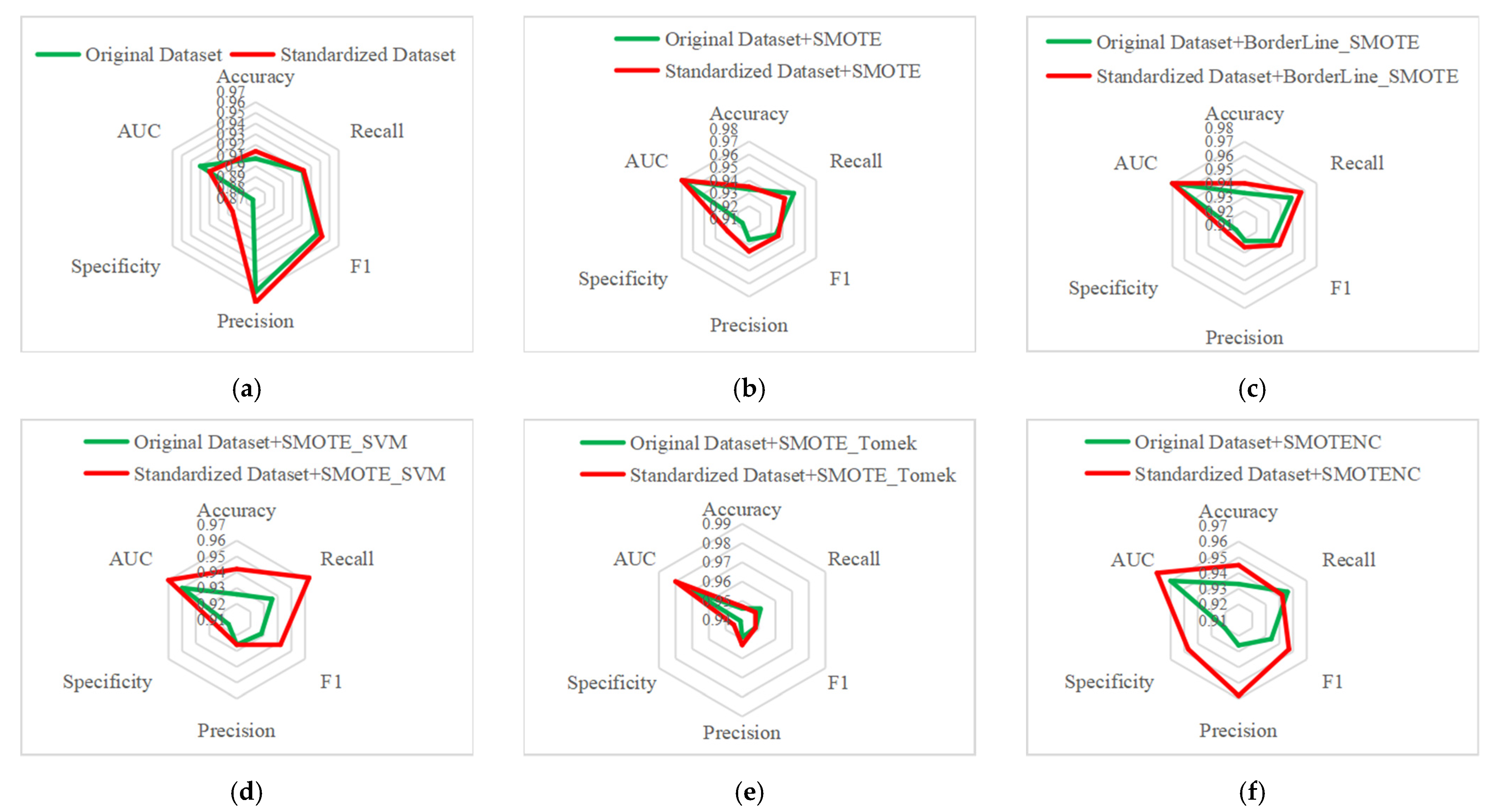
Figure 31.
The performance comparison of lightGBM + lr model on six groups of datasets. (a–f) correspond to the datasets without balancing and the datasets processed by SMOTE, BorderLine_SMOTE, SMOTE_SVM, SMOTE_Tomek and SMOTENC, respectively.
Figure 31.
The performance comparison of lightGBM + lr model on six groups of datasets. (a–f) correspond to the datasets without balancing and the datasets processed by SMOTE, BorderLine_SMOTE, SMOTE_SVM, SMOTE_Tomek and SMOTENC, respectively.
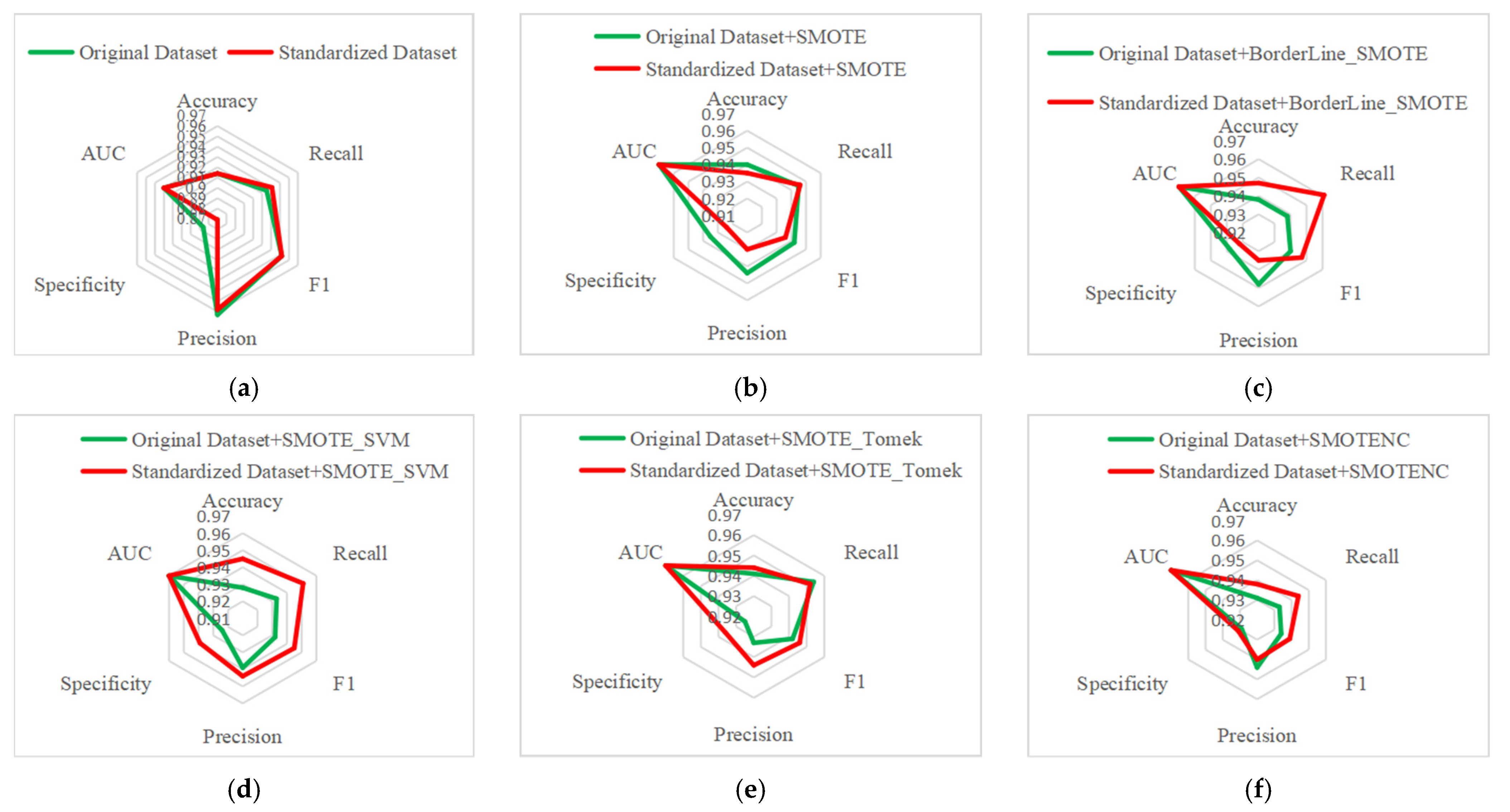
Figure 32.
The performance comparison of lightGBM + LR model on six groups of datasets. (a–f) correspond to the datasets without balancing and the datasets processed by SMOTE, BorderLine_SMOTE, SMOTE_SVM, SMOTE_Tomek and SMOTENC, respectively.
Figure 32.
The performance comparison of lightGBM + LR model on six groups of datasets. (a–f) correspond to the datasets without balancing and the datasets processed by SMOTE, BorderLine_SMOTE, SMOTE_SVM, SMOTE_Tomek and SMOTENC, respectively.
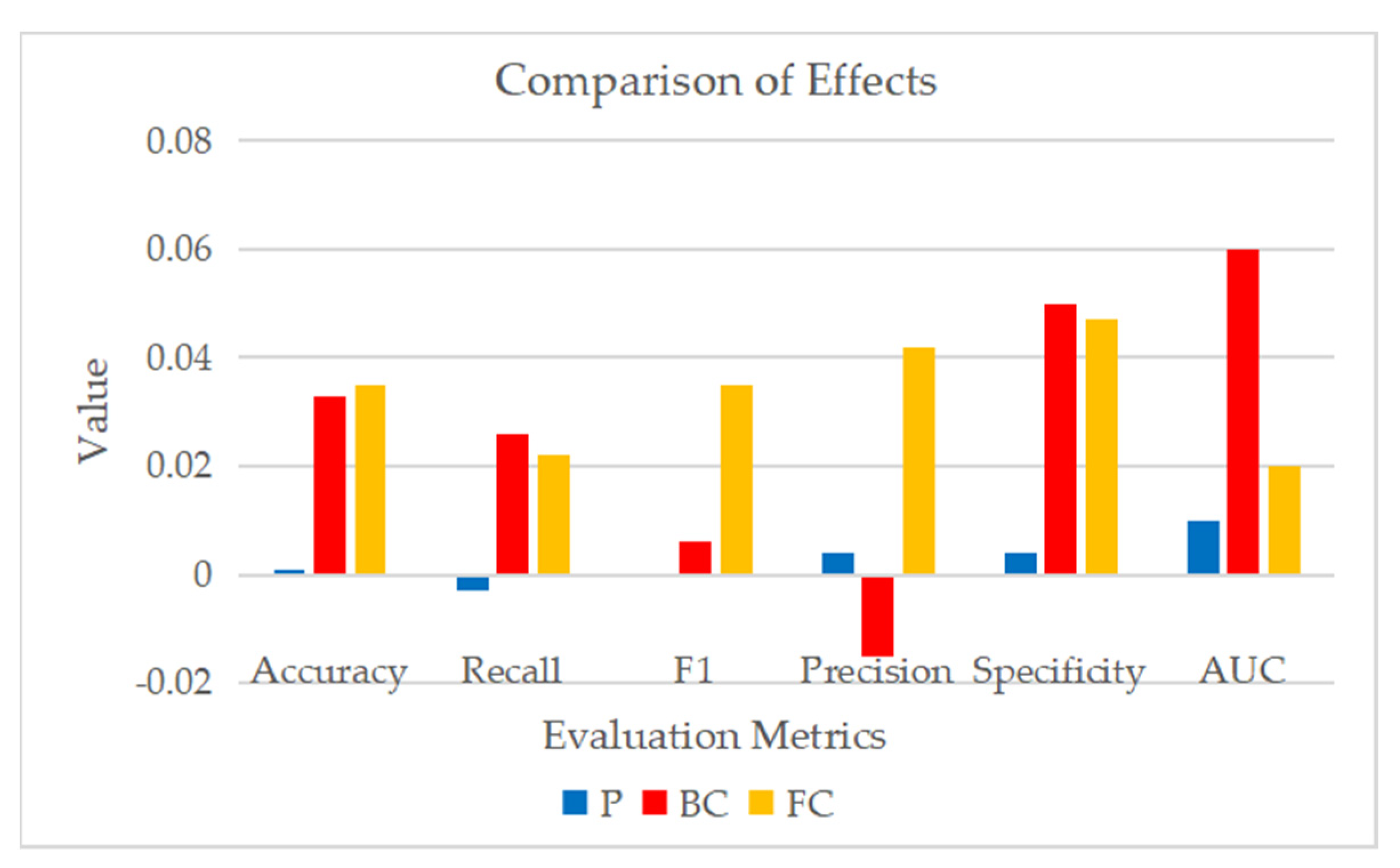
Figure 33.
Comparison of improvement effects of different modules on performance results.
Figure 33.
Comparison of improvement effects of different modules on performance results.
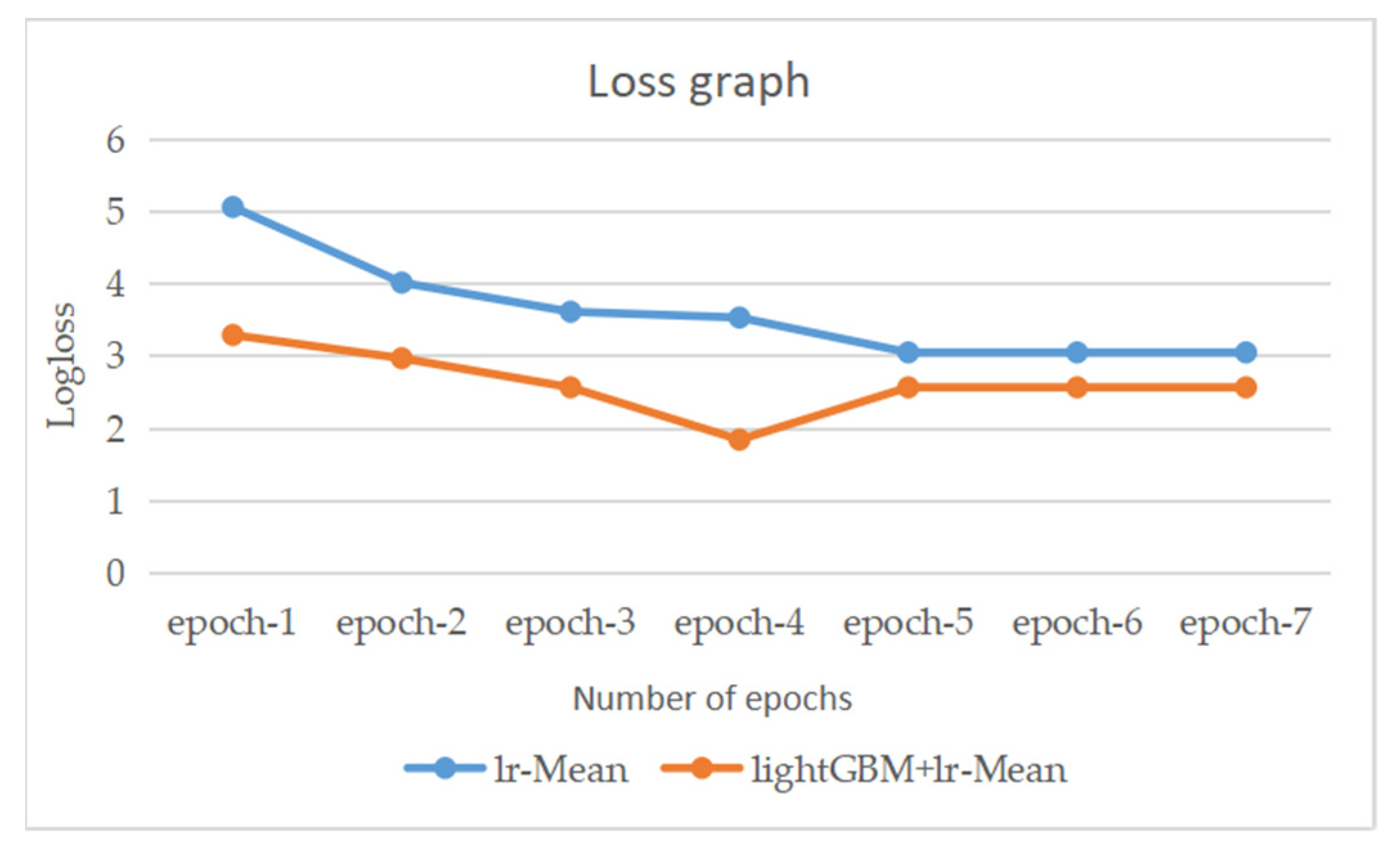
Figure 34.
The change trend of the loss of the two models on the training set.
Figure 34.
The change trend of the loss of the two models on the training set.
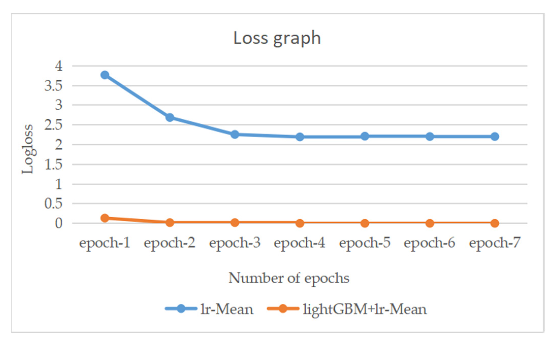
Figure 35.
The change trend of the loss of the two models on the test set.
Figure 35.
The change trend of the loss of the two models on the test set.
Table 1.
Top three causes of whole world DALYs and percentage of all DALYs in 2019.
Table 1.
Top three causes of whole world DALYs and percentage of all DALYs in 2019.
| Order | Causes 1 | Percentag 1 | Causes 2 | Percentag 2 | Causes 3 | Percentag 3 | Causes 4 | Percentag 4 |
|---|
| 1 | Neonatal disorders | 7.3 | Road injuries | 5.1 | IHD | 11.8 | IHD | 16.2 |
| 2 | IHD | 7.2 | HIV/AIDS | 4.8 | Stroke | 9.3 | Stroke | 13.0 |
| 3 | Stroke | 5.7 | IHD | 4.7 | Diabetes | 5.1 | COPD | 8.5 |
Table 2.
Detailed information of each feature and feature attribute in Z-Alizadeh Sani dataset.
Table 2.
Detailed information of each feature and feature attribute in Z-Alizadeh Sani dataset.
| Category | Feature Name | Range | Type |
|---|
| Demographic features | Age | 30–86 | continuous |
| | Weight | 48–120 | continuous |
| Length | 140–188 | continuous |
| Sex | Male, Female | categorical |
| BMI | 18.12–40.90 | continuous |
| DM | 0, 1 | categorical |
| HTN | 0, 1 | categorical |
| Current smoker | 0, 1 | categorical |
| Ex-smoker | 0, 1 | categorical |
| FH | 0, 1 | categorical |
| Obesity (Yes (BMI > 25), else No) | Y, N | categorical |
| CRF | Y, N | categorical |
| CVA | Y, N | categorical |
| Airway disease | Y, N | categorical |
| Thyroid disease | Y, N | categorical |
| CHF | Y, N | categorical |
| DLP | Y, N | categorical |
| Symptoms and Physical examination | BP | 90.0–190.0 | continuous |
| PR | 50.0–110.0 | continuous |
| | Edema | 0, 1 | categorical |
| Weak peripheral pulse | Y, N | categorical |
| Lung rales | Y, N | categorical |
| Systolic murmur | Y, N | categorical |
| Diastolic murmur | Y, N | categorical |
| Typical chest pain | 0, 1 | categorical |
| Dyspnea | Y, N | categorical |
| Function class | 1–4 | categorical |
| Atypical | Y, N | categorical |
| Nonanginal | Y, N | categorical |
| Exertional CP | N | categorical |
| LowTH Ang | Y, N | categorical |
| Electrocardiography | Q Wave | 0, 1 | categorical |
| | St elevation | 0, 1 | categorical |
| St depression | 0, 1 | categorical |
| T inversion | 0, 1 | categorical |
| LVH | Y, N | categorical |
| Poor R progression | Y, N | categorical |
| BBB | N, LBBB, RBBB | categorical |
| Laboratory Tests and Echocardiography | FBS | 62.0–400.0 | continuous |
| CR | 0.5–2.2 | continuous |
| | TG | 37.0–1050.0 | continuous |
| LDL | 18.0–232.0 | continuous |
| HDL | 15.9–111.0 | continuous |
| BUN | 6.0–52.0 | continuous |
| ESR | 1–90 | continuous |
| HB | 8.9–17.6 | continuous |
| K | 3.0–6.6 | continuous |
| Na | 128.0–156.0 | continuous |
| WBC | 3700–18,000 | continuous |
| Lymph | 7.0–60.0 | continuous |
| Neut | 32.0–89.0 | continuous |
| PLT | 25.0–742.0 | continuous |
| EF-TTE | 15.0–60.0 | continuous |
| Region RWMA | 0, 1, 2, 3, 4 | categorical |
| VHD | Mild, N, moderate, severe | categorical |
Table 3.
Statistical description of continuous features of Z-Alizadeh Sani dataset.
Table 3.
Statistical description of continuous features of Z-Alizadeh Sani dataset.
| Feature | Min | Max | Ave | Med | 1th | 5th | 10th | 50th | 90th | 95th | 99th |
|---|
| Age | 30 | 86 | 58.9 | 58.00 | 36.08 | 43.00 | 47.00 | 58.00 | 73.00 | 76.00 | 81.00 |
| Weight | 48 | 120 | 73.83 | 74.00 | 50.00 | 55.00 | 60.00 | 74.00 | 89.00 | 94.80 | 107.88 |
| Length | 140 | 188 | 164.72 | 165.00 | 145.00 | 150.00 | 152.00 | 165.00 | 176.60 | 179.00 | 185.96 |
| BMI | 18.12 | 40.90 | 27.25 | 26.78 | 18.83 | 21.10 | 22.31 | 26.78 | 33.21 | 34.88 | 38.24 |
| BP | 90 | 190 | 129.55 | 130.00 | 90.00 | 100.00 | 110.00 | 130.00 | 160.00 | 160.00 | 180.00 |
| PR | 50 | 110 | 75.14 | 70.00 | 60.00 | 64.00 | 70.00 | 70.00 | 87.20 | 90.00 | 109.60 |
| FBS | 62 | 400 | 119.18 | 98.00 | 69.04 | 77.00 | 80.00 | 98.00 | 193.20 | 223.80 | 358.40 |
| CR | 0.50 | 2.20 | 1.06 | 1.00 | 0.60 | 0.70 | 0.80 | 1.00 | 1.40 | 1.50 | 1.90 |
| TG | 37 | 1050 | 150.34 | 122.00 | 43.12 | 67.40 | 76.00 | 122.00 | 250.00 | 309.00 | 469.20 |
| LDL | 18 | 232 | 104.64 | 100.00 | 30.24 | 52.60 | 64.40 | 100.00 | 154.20 | 170.00 | 212.60 |
| HDL | 15.9 | 111.0 | 40.23 | 39.00 | 18.16 | 25.20 | 28.00 | 39.00 | 53.00 | 55.80 | 81.40 |
| BUN | 6 | 52 | 17.50 | 16.00 | 8.00 | 10.00 | 11.00 | 16.00 | 25.60 | 31.80 | 42.92 |
| ESR | 1 | 90 | 19.46 | 15.00 | 1.04 | 3.00 | 4.00 | 15.00 | 41.00 | 51.00 | 79.84 |
| HB | 8.9 | 17.6 | 13.15 | 13.20 | 9.00 | 10.02 | 11.00 | 13.20 | 15.10 | 15.68 | 17.19 |
| K | 3.0 | 6.6 | 4.23 | 4.20 | 3.20 | 3.50 | 3.70 | 4.20 | 4.80 | 5.00 | 5.40 |
| Na | 128 | 156 | 141.00 | 141.00 | 130.04 | 135.00 | 137.00 | 141.00 | 145.00 | 147.00 | 153.00 |
| WBC | 3700 | 18,000 | 7562.05 | 7100.00 | 3812.00 | 4700.00 | 5100.00 | 7100.00 | 10,700.00 | 12,100.00 | 16,960.00 |
| Lymph | 7 | 60 | 32.40 | 32.00 | 9.04 | 15.20 | 19.00 | 32.00 | 44.00 | 49.00 | 58.96 |
| Neut | 32 | 89 | 60.15 | 60.00 | 35.12 | 44.00 | 49.00 | 60.00 | 73.60 | 78.00 | 84.96 |
| PLT | 25 | 742 | 221.49 | 210.00 | 118.44 | 158.20 | 170.00 | 210.00 | 293.60 | 331.60 | 391.52 |
| EF-TTE | 15 | 60 | 47.23 | 50.00 | 20.00 | 26.00 | 35.00 | 50.00 | 55.00 | 55.00 | 60.00 |
Table 4.
The performance results obtained by the five models on the original dataset.
Table 4.
The performance results obtained by the five models on the original dataset.
| Algorithms | Accuracy | Recall | F1 | Precision | Specificity | AUC |
|---|
| RF | 0.887 ± 0.056 | 0.909 ± 0.051 | 0.923 ± 0.038 | 0.940 ± 0.051 | 0.834 ± 0.117 | 0.92 ± 0.05 |
| Extratrees | 0.891 ± 0.045 | 0.932 ± 0.045 | 0.923 ± 0.033 | 0.916 ± 0.055 | 0.788 ± 0.123 | 0.91 ± 0.06 |
| AdaBoost | 0.904 ± 0.059 | 0.929 ± 0.067 | 0.934 ± 0.038 | 0.944 ± 0.050 | 0.842 ± 0.111 | 0.93 ± 0.05 |
| XGBoost | 0.894 ± 0.068 | 0.909 ± 0.072 | 0.929 ± 0.044 | 0.954 ± 0.046 | 0.856 ± 0.106 | 0.93 ± 0.05 |
| lightGBM | 0.911 ± 0.060 | 0.922 ± 0.068 | 0.940 ± 0.038 | 0.963 ± 0.041 | 0.881 ± 0.095 | 0.93 ± 0.05 |
Table 5.
Confusion matrix.
Table 5.
Confusion matrix.
| | | |
| TN | FP |
| FN | TP |
Table 6.
The average results of 10 tests obtained by classification models on the source dataset.
Table 6.
The average results of 10 tests obtained by classification models on the source dataset.
| Classifiers | Accuracy | Recall | F1 | Precision | Specificity | AUC |
|---|
| lightGBM | 0.911 ± 0.060 | 0.922 ± 0.068 | 0.940 ± 0.038 | 0.963 ± 0.041 | 0.881 ± 0.095 | 0.93 ± 0.05 |
| lr | 0.884 ± 0.052 | 0.911 ± 0.059 | 0.921 ± 0.032 | 0.935 ± 0.042 | 0.819 ± 0.099 | 0.93 ± 0.05 |
| lightGBM + lr | 0.907 ± 0.047 | 0.921 ± 0.059 | 0.937 ± 0.028 | 0.958 ± 0.038 | 0.873 ± 0.081 | 0.93 ± 0.06 |
| lightGBM + LR | 0.914 ± 0.045 | 0.925 ± 0.059 | 0.942 ± 0.029 | 0.963 ± 0.035 | 0.886 ± 0.074 | 0.93 ± 0.05 |
Table 7.
The average results of 10 tests obtained by classification models on the dataset processed by SMOTE.
Table 7.
The average results of 10 tests obtained by classification models on the dataset processed by SMOTE.
| Classifiers | Accuracy | Recall | F1 | Precision | Specificity | AUC |
|---|
| lightGBM | 0.931 ± 0.055 | 0.930 ± 0.090 | 0.934 ± 0.048 | 0.944 ± 0.035 | 0.932 ± 0.039 | 0.96 ± 0.03 |
| lr | 0.915 ± 0.057 | 0.932 ± 0.096 | 0.917 ± 0.049 | 0.911 ± 0.058 | 0.897 ± 0.047 | 0.96 ± 0.03 |
| lightGBM + lr | 0.933 ± 0.054 | 0.950 ± 0.083 | 0.934 ± 0.047 | 0.926 ± 0.052 | 0.916 ± 0.053 | 0.97 ± 0.04 |
| lightGBM + LR | 0.940 ± 0.048 | 0.945 ± 0.078 | 0.942 ± 0.043 | 0.944 ± 0.041 | 0.935 ± 0.037 | 0.97 ± 0.03 |
Table 8.
The average results of 10 tests obtained by classification models on the dataset processed by Borderline_SMOTE.
Table 8.
The average results of 10 tests obtained by classification models on the dataset processed by Borderline_SMOTE.
| Classifiers | Accuracy | Recall | F1 | Precision | Specificity | AUC |
|---|
| lightGBM | 0.933 ± 0.041 | 0.938 ± 0.081 | 0.935 ± 0.035 | 0.939 ± 0.042 | 0.928 ± 0.033 | 0.97 ± 0.03 |
| lr | 0.903 ± 0.052 | 0.919 ± 0.087 | 0.904 ± 0.046 | 0.897 ± 0.059 | 0.887 ± 0.049 | 0.96 ± 0.03 |
| lightGBM + lr | 0.933 ± 0.047 | 0.949 ± 0.068 | 0.933 ± 0.046 | 0.921 ± 0.057 | 0.917 ± 0.056 | 0.97 ± 0.03 |
| lightGBM + LR | 0.938 ± 0.053 | 0.938 ± 0.081 | 0.940 ± 0.048 | 0.948 ± 0.058 | 0.938 ± 0.058 | 0.97 ± 0.03 |
Table 9.
The average results of 10 tests obtained by classification models on the dataset processed by SMOTE_SVM.
Table 9.
The average results of 10 tests obtained by classification models on the dataset processed by SMOTE_SVM.
| Classifiers | Accuracy | Recall | F1 | Precision | Specificity | AUC |
|---|
| lightGBM | 0.931 ± 0.052 | 0.937 ± 0.084 | 0.933 ± 0.046 | 0.935 ± 0.043 | 0.925 ± 0.044 | 0.97 ± 0.03 |
| lr | 0.903 ± 0.059 | 0.926 ± 0.087 | 0.903 ± 0.055 | 0.888 ± 0.068 | 0.880 ± 0.062 | 0.95 ± 0.04 |
| lightGBM + lr | 0.926 ± 0.059 | 0.936 ± 0.087 | 0.928 ± 0.052 | 0.926 ± 0.043 | 0.916 ± 0.050 | 0.95 ± 0.04 |
| lightGBM + LR | 0.928 ± 0.062 | 0.933 ± 0.098 | 0.932 ± 0.054 | 0.939 ± 0.047 | 0.924 ± 0.049 | 0.96 ± 0.03 |
Table 10.
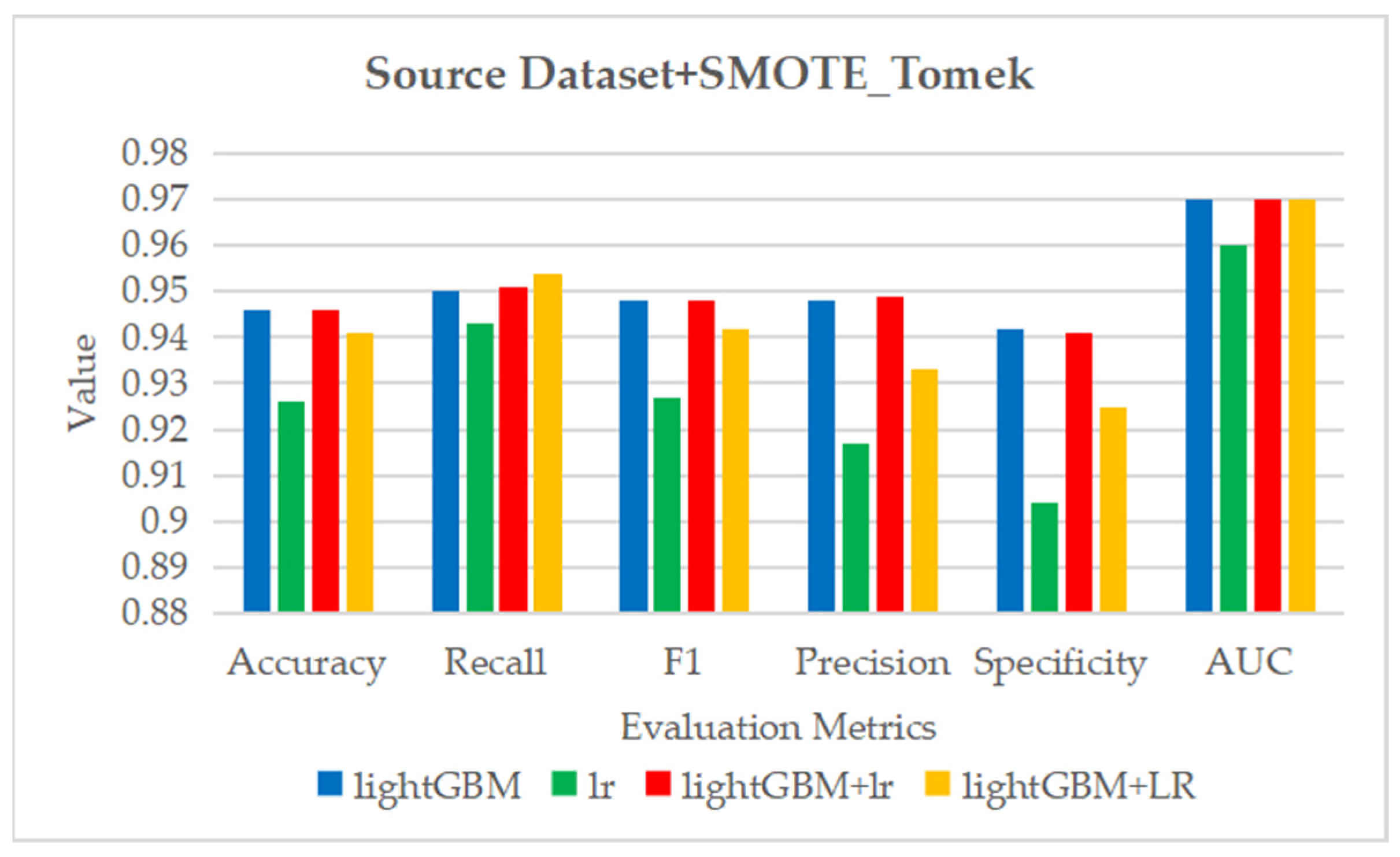
The average results of 10 tests obtained by classification models on the dataset processed by SMOTE_Tomek.
Table 10.
The average results of 10 tests obtained by classification models on the dataset processed by SMOTE_Tomek.
| Classifiers | Accuracy | Recall | F1 | Precision | Specificity | AUC |
|---|
| lightGBM | 0.946 ± 0.044 | 0.950 ± 0.065 | 0.948 ± 0.040 | 0.948 ± 0.040 | 0.942 ± 0.044 | 0.97 ± 0.03 |
| lr | 0.926 ± 0.051 | 0.943 ± 0.083 | 0.927 ± 0.044 | 0.917 ± 0.043 | 0.904 ± 0.046 | 0.96 ± 0.04 |
| lightGBM + lr | 0.946 ± 0.049 | 0.951 ± 0.071 | 0.948 ± 0.045 | 0.949 ± 0.040 | 0.941 ± 0.045 | 0.97 ± 0.04 |
| lightGBM + LR | 0.941 ± 0.038 | 0.954 ± 0.064 | 0.942 ± 0.034 | 0.933 ± 0.034 | 0.925 ± 0.036 | 0.97 ± 0.04 |
Table 11.
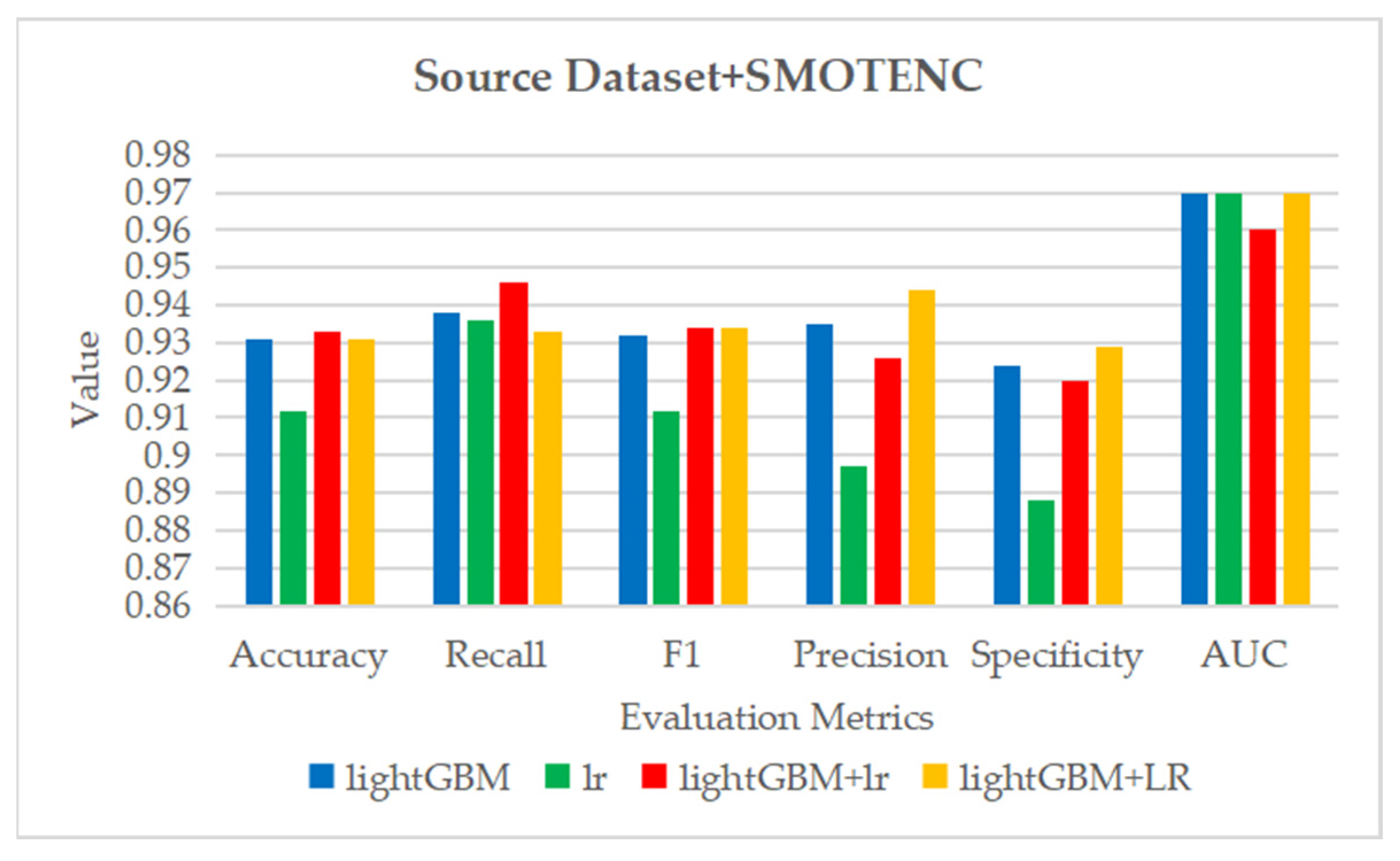
The average results of 10 tests obtained by classification models on the dataset processed by SMOTENC.
Table 11.
The average results of 10 tests obtained by classification models on the dataset processed by SMOTENC.
| Classifiers | Accuracy | Recall | F1 | Precision | Specificity | AUC |
|---|
| lightGBM | 0.931 ± 0.040 | 0.938 ± 0.080 | 0.932 ± 0.035 | 0.935 ± 0.052 | 0.924 ± 0.043 | 0.97 ± 0.03 |
| lr | 0.912 ± 0.051 | 0.936 ± 0.087 | 0.912 ± 0.046 | 0.897 ± 0.060 | 0.888 ± 0.054 | 0.97 ± 0.02 |
| lightGBM + lr | 0.933 ± 0.048 | 0.946 ± 0.075 | 0.934 ± 0.044 | 0.926 ± 0.037 | 0.920 ± 0.039 | 0.96 ± 0.04 |
| lightGBM + LR | 0.931 ± 0.052 | 0.933 ± 0.092 | 0.934 ± 0.044 | 0.944 ± 0.046 | 0.929 ± 0.038 | 0.97 ± 0.03 |
Table 12.
The average results of 10 tests obtained by classification models on the dataset processed by data standardization.
Table 12.
The average results of 10 tests obtained by classification models on the dataset processed by data standardization.
| Classifiers | Accuracy | Recall | F1 | Precision | Specificity | AUC |
|---|
| lightGBM | 0.897 ± 0.049 | 0.909 ± 0.058 | 0.931 ± 0.030 | 0.958 ± 0.044 | 0.869 ± 0.093 | 0.92 ± 0.06 |
| lr | 0.884 ± 0.059 | 0.900 ± 0.062 | 0.922 ± 0.037 | 0.949 ± 0.045 | 0.844 ± 0.105 | 0.93 ± 0.06 |
| lightGBM + lr | 0.914 ± 0.040 | 0.922 ± 0.058 | 0.942 ± 0.025 | 0.968 ± 0.036 | 0.895 ± 0.074 | 0.92 ± 0.06 |
| lightGBM + LR | 0.914 ± 0.060 | 0.931 ± 0.074 | 0.942 ± 0.038 | 0.958 ± 0.038 | 0.871 ± 0.086 | 0.93 ± 0.06 |
Table 13.
The average results of 10 tests obtained by classification models on the dataset processed by data standardization and SMOTE.
Table 13.
The average results of 10 tests obtained by classification models on the dataset processed by data standardization and SMOTE.
| Classifiers | Accuracy | Recall | F1 | Precision | Specificity | AUC |
|---|
| lightGBM | 0.924 ± 0.067 | 0.931 ± 0.100 | 0.927 ± 0.058 | 0.930 ± 0.043 | 0.917 ± 0.048 | 0.97 ± 0.03 |
| lr | 0.912 ± 0.049 | 0.923 ± 0.081 | 0.913 ± 0.044 | 0.911 ± 0.058 | 0.902 ± 0.053 | 0.96 ± 0.03 |
| lightGBM + lr | 0.935 ± 0.035 | 0.942 ± 0.066 | 0.936 ± 0.033 | 0.935 ± 0.038 | 0.929 ± 0.035 | 0.97 ± 0.03 |
| lightGBM + LR | 0.935 ± 0.045 | 0.946 ± 0.071 | 0.936 ± 0.042 | 0.930 ± 0.049 | 0.924 ± 0.049 | 0.97 ± 0.03 |
Table 14.
The average results of 10 tests obtained by classification models on the dataset processed by data standardization and Borderline_SMOTE.
Table 14.
The average results of 10 tests obtained by classification models on the dataset processed by data standardization and Borderline_SMOTE.
| Classifiers | Accuracy | Recall | F1 | Precision | Specificity | AUC |
|---|
| lightGBM | 0.935 ± 0.048 | 0.944 ± 0.079 | 0.937 ± 0.044 | 0.935 ± 0.048 | 0.926 ± 0.044 | 0.97 ± 0.03 |
| lr | 0.914 ± 0.052 | 0.934 ± 0.081 | 0.914 ± 0.048 | 0.902 ± 0.065 | 0.895 ± 0.064 | 0.96 ± 0.02 |
| lightGBM + lr | 0.940 ± 0.036 | 0.957 ± 0.054 | 0.939 ± 0.035 | 0.926 ± 0.048 | 0.923 ± 0.047 | 0.97 ± 0.03 |
| lightGBM + LR | 0.947 ± 0.036 | 0.961 ± 0.054 | 0.947 ± 0.034 | 0.935 ± 0.043 | 0.932 ± 0.042 | 0.97 ± 0.03 |
Table 15.
The average results of 10 tests obtained by classification models on the dataset processed by data standardization and SMOTE_SVM.
Table 15.
The average results of 10 tests obtained by classification models on the dataset processed by data standardization and SMOTE_SVM.
| Classifiers | Accuracy | Recall | F1 | Precision | Specificity | AUC |
|---|
| lightGBM | 0.938 ± 0.058 | 0.944 ± 0.080 | 0.939 ± 0.052 | 0.939 ± 0.052 | 0.932 ± 0.056 | 0.97 ± 0.03 |
| lr | 0.917 ± 0.047 | 0.936 ± 0.082 | 0.917 ± 0.043 | 0.906 ± 0.061 | 0.898 ± 0.056 | 0.96 ± 0.03 |
| lightGBM + lr | 0.942 ± 0.040 | 0.963 ± 0.065 | 0.942 ± 0.037 | 0.926 ± 0.038 | 0.922 ± 0.037 | 0.96 ± 0.04 |
| lightGBM + LR | 0.945 ± 0.036 | 0.951 ± 0.062 | 0.945 ± 0.033 | 0.944 ± 0.041 | 0.939 ± 0.036 | 0.96 ± 0.03 |
Table 16.
The average results of 10 tests obtained by classification models on the dataset processed by data standardization and SMOTE_Tomek.
Table 16.
The average results of 10 tests obtained by classification models on the dataset processed by data standardization and SMOTE_Tomek.
| Classifiers | Accuracy | Recall | F1 | Precision | Specificity | AUC |
|---|
| lightGBM | 0.937 ± 0.048 | 0.939 ± 0.085 | 0.940 ± 0.041 | 0.948 ± 0.039 | 0.936 ± 0.032 | 0.98 ± 0.02 |
| lr | 0.912 ± 0.051 | 0.926 ± 0.089 | 0.913 ± 0.045 | 0.911 ± 0.066 | 0.898 ± 0.055 | 0.96 ± 0.03 |
| lightGBM + lr | 0.947 ± 0.050 | 0.948 ± 0.073 | 0.948 ± 0.046 | 0.953 ± 0.047 | 0.945 ± 0.048 | 0.98 ± 0.02 |
| lightGBM + LR | 0.944 ± 0.048 | 0.952 ± 0.075 | 0.946 ± 0.043 | 0.944 ± 0.046 | 0.936 ± 0.045 | 0.97 ± 0.03 |
Table 17.
The average results of 10 tests obtained by classification models on the dataset processed by data standardization and SMOTENC.
Table 17.
The average results of 10 tests obtained by classification models on the dataset processed by data standardization and SMOTENC.
| Classifiers | Accuracy | Recall | F1 | Precision | Specificity | AUC |
|---|
| lightGBM | 0.931 ± 0.058 | 0.934 ± 0.089 | 0.933 ± 0.052 | 0.939 ± 0.056 | 0.928 ± 0.055 | 0.97 ± 0.03 |
| lr | 0.917 ± 0.046 | 0.926 ± 0.086 | 0.919 ± 0.042 | 0.921 ± 0.061 | 0.908 ± 0.052 | 0.96 ± 0.03 |
| lightGBM + lr | 0.945 ± 0.050 | 0.942 ± 0.080 | 0.947 ± 0.045 | 0.958 ± 0.049 | 0.947 ± 0.047 | 0.97 ± 0.03 |
| lightGBM + LR | 0.938 ± 0.043 | 0.944 ± 0.074 | 0.939 ± 0.040 | 0.940 ± 0.055 | 0.931 ± 0.050 | 0.97 ± 0.02 |
Table 18.
The classification results of the prediction model after removing the modules of data preprocessing.
Table 18.
The classification results of the prediction model after removing the modules of data preprocessing.
| Modules | Accuracy | Recall | F1 | Precision | Specificity | AUC |
|---|
| ALL | 0.947 ± 0.050 | 0.948 ± 0.073 | 0.948 ± 0.046 | 0.953 ± 0.047 | 0.945 ± 0.048 | 0.98 ± 0.02 |
| NP | 0.946 ± 0.049 | 0.951 ± 0.071 | 0.948 ± 0.045 | 0.949 ± 0.040 | 0.941 ± 0.045 | 0.97 ± 0.04 |
| P | 0.001 | −0.003 | 0.000 | 0.004 | 0.004 | 0.01 |
Table 19.
The classification results of the prediction model after removing the modules of class balance processing.
Table 19.
The classification results of the prediction model after removing the modules of class balance processing.
| Modules | Accuracy | Recall | F1 | Precision | Specificity | AUC |
|---|
| ALL | 0.947 ± 0.050 | 0.948 ± 0.073 | 0.948 ± 0.046 | 0.953 ± 0.047 | 0.945 ± 0.048 | 0.98 ± 0.02 |
| NBC | 0.914 ± 0.040 | 0.922 ± 0.058 | 0.942 ± 0.025 | 0.968 ± 0.036 | 0.895 ± 0.074 | 0.92 ± 0.06 |
| BC | 0.033 | 0.026 | 0.006 | −0.015 | 0.050 | 0.06 |
Table 20.
The classification results of the prediction model after removing the modules of feature combination.
Table 20.
The classification results of the prediction model after removing the modules of feature combination.
| Modules | Accuracy | Recall | F1 | Precision | Specificity | AUC |
|---|
| ALL | 0.947 ± 0.050 | 0.948 ± 0.073 | 0.948 ± 0.046 | 0.953 ± 0.047 | 0.945 ± 0.048 | 0.98 ± 0.02 |
| NFC | 0.912 ± 0.051 | 0.926 ± 0.089 | 0.913 ± 0.045 | 0.911 ± 0.066 | 0.898 ± 0.055 | 0.96 ± 0.03 |
| FC | 0.035 | 0.022 | 0.035 | 0.042 | 0.047 | 0.02 |
Table 21.
The comparison of classification results between our study and other studies on the Z-Alizadeh Sani dataset.
Table 21.
The comparison of classification results between our study and other studies on the Z-Alizadeh Sani dataset.
| Method | Accuracy % | Recall % | F1% | Precision % | Specificity % | AUC |
|---|
| SMO [33] | 92.09 | 97.22 | N | N | 79.31 | N |
| SMO + IG [30] | 94.08 | 96.30 | N | N | 88.51 | N |
| KNN [43] | 90.91 | 93.33 | 93.33 | 93.33 | 85.71 | N |
| NN + genetic algorithm [32] | 93.85 | 97 | N | N | 92 | N |
| NB + genetic algorithm [69] | 88.16 | 88.00 | N | N | 87.78 | N |
| Ensemble [70] | 86.49 | 73.61 | 0.75 | N | 91.67 | 0.83 |
| SVM + feature engineering + 500 examples [37] | 96.4 | 100 | N | N | 88.1 | 0.92 |
| NE-nu-SVC [35] | 94.66 | 94.70 | 94.70 | 94.70 | N | 0.966 |
| N2GC-nuSVM [36] | 93.08 | N | 91.51 | N | N | N |
| XGBoost + hybrid FSA + FA + ETCA + SMOTE [31] | 92.58 | 92.99 | 90.62 | 92.59 | N | N |
| Hybrid PSO-EmNN coupled with feature selection [38] | 88.34 | 91.85 | 92.12 | 92.37 | 78.98 | N |
| XGBoost + feature construction + SMOTE [48] | 94.7 | 96.1 | 94.6 | 93.4 | 93.2 | 0.98 |
| GSVMA [47] | 89.45 | 81.22 | 80.49 | N | 100 | 100 |
| C-CADZ [41] | 97.37 | 98.15 | N | N | 95.45 | N |
| CART [46] | 92.41 | 98.61 | N | N | 77.01 | N |
| lightGBM + lr + SMOTE_Tomek * | 94.7 | 94.8 | 94.8 | 95.3 | 94.5 | 0.98 |


