Less Is More: Robust and Novel Features for Malicious Domain Detection

Abstract

Malicious domains are increasingly common and pose a severe cybersecurity threat. Specifically, many types of current cyber attacks use URLs for attack communications (e.g., C&C, phishing, and spear-phishing). Despite the continuous progress in detecting cyber attacks, there are still critical weak spots in the structure of defense mechanisms. Since machine learning has become one of the most prominent malware detection methods, a robust feature selection mechanism is proposed that results in malicious domain detection models that are resistant to evasion attacks. This mechanism exhibits a high performance based on empirical data. This paper makes two main contributions: First, it provides an analysis of robust feature selection based on widely used features in the literature. Note that even though the feature set dimensional space is cut by half, the performance of the classifier is still improved (an increase in the model’s F1-score from 92.92% to 95.81%). Second, it introduces novel features that are robust with regard to the adversary’s manipulation. Based on an extensive evaluation of the different feature sets and commonly used classification models, this paper shows that models based on robust features are resistant to malicious perturbations and concurrently are helpful in classifying non-manipulated data.

1. Introduction

Cybersecurity attacks have become a significant issue for governments and civilians [1]. Many of these attacks are based on malicious web domains or URLs (see Figure 1 for an example of a URL structure). These domains are used for phishing [2,3,4,5,6] (e.g., spear phishing), Command and Control (C&C) [7] and a vast set of virus and malware [8] attacks. Therefore, the ability to identify a malicious domain in advance is a massive game-changer [9,10,11,12,13,14,15,16,17,18,19,20,21,22,23,24,25,26].

A common way of identifying malicious/compromised domains is to collect information about the domain names (alphanumeric characters) and network information (such as DNS and passive DNS data). This information is then used to extract a set of features, according to which machine learning (ML) algorithms are trained based on a massive amount of data [11,12,13,14,15,17,18,19,20,21,22,24,26,27,28]. A mathematical approach can also be used in various ways [16,26], such as measuring the distance between a known malicious domain name and the analyzed domain (benign or malicious) [26]. Nonetheless, while ML-based solutions are widely used, many of them are not robust; an attacker can easily bypass these models with minimal feature perturbations (e.g., changing the domain’s length or modifying network parameters such as Time To Live (TTL)) [29,30]. In this context, one of the main problems is how to train a robust malicious domain classifier, one that is immune to the presence of an intelligent adversary that can manipulate domain properties, to classify malicious domains as benign.

For this purpose, a feature selection process is executed to differentiate between robust and non-robust features. Given the robust feature set, the defender is still guaranteed to provide an efficient classifier, which is harder to manipulate. Even if the attacker has black-box access to the model, tampering with the domain properties or network parameters will have a negligible effect on the classifier’s accuracy. In order to achieve this goal, we collected a broad set of both malicious and benign URLs. In addition, we reviewed related work and identified a set of features commonly used for the classification task. These features were then artificially manipulated to show that some, although widely used, are not robust in the face of adversarial perturbations. In a complementary manner, we engineered an original set of novel and robust features. Therefore, we created a hybrid set of features, combining the robust well-known features with our novel features. Finally, the different feature sets (e.g., common, robust common, and novel) were evaluated using common machine learning algorithms, with emphasis on the importance of feature selection and feature engineering processes.

The rest of the paper is organized as follows: Section 2 summarizes related work. Section 3 describes the methodology and the novel features. Section 4 presents the empirical analysis and evaluation. Finally, Section 5 concludes and summarizes this work.

2. Related Work

The issue of identifying malicious domains is a fundamental problem in cybersecurity. This section discusses recent results in identifying malicious domains, focusing on two significant methodologies, mathematical theory (MT) approaches and machine learning (ML)-based techniques.

The use of graph theory to identify malicious domains was more pervasive in the past [16,26,31,32,33]. Yadav et al. [26] presented a method for recognizing malicious domain names based on fast flux. Fast flux is a DNS technique used by botnets to hide phishing and malware delivery sites behind an ever-changing network of compromised hosts acting as proxies. They analyzed the DNS queries and responses to detect if and when domain names were being generated by a Domain Generation Algorithm (DGA). Their solution was based on computing the distribution of alphanumeric characters for groups of domains and by statistical metrics with the KL (Kullback Leibler) distance, Edit distance and Jaccard measure to identify these domains. For a fast-flux attack using the Jaccard Index, they achieved impressive results, with 100% detection and 0% false positives. However, for smaller numbers of generated domains for each TLD, their false-positive results were much higher, at 15% when 50 domains were generated for the TLD using the KL-divergence over unigrams, and 8% when 200 domains were generated for each TLD using the Edit distance.

Dolberg et al. [16] described a system called Multi-dimensional Aggregation Monitoring (MAM) that detects anomalies in DNS data by measuring and comparing a “steadiness” metric over time for domain names and IP addresses using a tree-based mechanism. The steadiness metric is based on a domain similar to IP resolution patterns when comparing DNS data over a sequence of consecutive time frames. The domain name to IP mappings were based on an aggregation scheme and measured steadiness. In terms of detecting malicious domains, the results showed that an average steadiness value of 0.45 could be used as a reasonable threshold value, with a 73% true positive rate and only a 0.3% false positive one. The steadiness values might not be considered a good indicator when fewer malicious activities are present (e.g., <10%).

However, the most common approach to identifying malicious domains is by means of machine learning (ML) and Deep Learning (DL) [11,14,20,23,24,27,28,34,35,36,37,38,39,40,41,42]. Researchers can train ML algorithms to label URLs as malicious or benign using a set of extracted features. Shi et al. [23] proposed a machine learning methodology to detect malicious domain names using the Extreme Learning Machine (ELM) [19], which is closest to the one employed here. ELM is a new neural network with a high accuracy and fast learning speed. The authors divided their features into four categories: construction-based, IP-based, TTL-based, and WHOIS-based categories. Their evaluation resulted in a high detection rate with an accuracy exceeding 95% and a fast learning speed. However, as shown below, a significant fraction of the features used in this work emerged as non-robust and ineffective in the presence of an intelligent adversary.

Sun et al. [24] presented a system called HinDom, which generates a heterogeneous graph (in contrast to homogeneous graphs created by Rahbarinia et al. [22] and Yadav et al. [26]) in order to robustly identify malicious attacks (e.g., spam, phishing, malware, and botnets). Even though HinDom collected DNS and pDNS data, it also has the ability to collect information from various clients inside networks (e.g., CERNET2 and TUNET); thus, its perspective is different from the perspective of this study (i.e., client perspective). Nevertheless, HinDom has achieved remarkable results using a transductive classifier and achieved a high accuracy and F1-scores of 99% and 97.5%, respectively.

Bilge et al. [13] created a system called Exposure, which is designed to detect malicious domain names. Their system uses passive DNS data collected over some time to extract features related to known malicious and benign domains. Passive DNS Replication [11,13,20,22,25,27,28] refers to the reconstruction of DNS zone data by recording and aggregating live DNS queries and responses. Passive DNS data can be collected without requiring the cooperation of zone administrators. The Exposure system is designed to detect malware- and spam-related domains. It can also detect malicious fast-flux and DGA-related domains based on their unique features. The system computes the following four sets of features from anonymized DNS records: (a) time-based features related to the periods and frequencies that a specific domain name was queried in; (b) DNS-answer-based features calculated according to the number of distinctive resolved IP addresses and domain names, the countries in which the IP addresses reside, and the ratio of the resolved IP addresses that can be matched with valid domain names and other services; (c) TTL-based features that are calculated based on a statistical analysis of the TTL over a given time series; and (d) domain name-based features that are extracted by computing the ratio of the numerical characters to the domain name string, and the ratio of the size of the longest meaningful substring in the domain name. Using a Decision Tree model, Exposure reported a total of 100,261 distinct domains as being malicious, which resulted in 19,742 unique IP addresses. The combination of features used to identify malicious domains led to the successful identification of several domains related to botnets, flux networks, and DGAs, with low false-positive and high detection rates. It may not be possible to generalize the detection rate results reported by the authors (98%) since they were highly dependent on comparisons with biased datasets. Despite the positive results, once an identification scheme is published, it is always possible for an attacker to evade detection by mimicking the behaviors of benign domains.

Rahbarinia et al. [22] presented a system called Segugio, which is an anomaly detection system based on passive DNS traffic to identify malware-controlled domain names based on their relationship to known malicious domains. The system detects malware-controlled domains by creating a machine domain bipartite graph representing the underlying relations between new domains and known benign/malicious domains. The system operates by calculating the following features: (a) machine behavior, based on the ratio of “known malicious” and “unknown” domains that query a given domain d over the total number of machines that query d. The larger the total number of queries and the fraction of malicious related queries, the higher the probability that d is a malware-controlled domain; (b) Domain activity, where given a time period, domain activity is computed by counting the total number of days in which a domain was actively queried; (c) IP abuse, where, given a set of IP addresses that the domain resolves to, this feature represents the fraction of those IP addresses that were previously targeted by known malware-controlled domains. Using a Random Forest model, Segugio was shown to produce high true positive and meager false positive rates (94% and 0.1%, respectively). It was also able to detect malicious domains earlier than commercial blacklisting websites. However, Segugio is a system that can only detect malware-related domains based on their relationship to previously known domains and therefore cannot detect new (unrelated to previous malicious domains) malicious domains. Additional information concerning malicious domain filtering and malicious URL detection can be found in [34,42].

Adversarial machine learning is a subfield of machine learning in which instances used to train the model and instances in the wild may be characterized by different distributions. For example, given perturbations on a malicious instance so that it will be falsely classified as benign. These manipulated instances are commonly called adversarial examples (AE) [43]. AE are samples that an attacker changes based on some model classification function knowledge. These examples are slightly different from correctly classified examples. Therefore, the model fails to classify them correctly. AE are widely used in the fields of spam filtering [44], network intrusion detection systems (IDS) [45], anti-virus signature tests [46] and biometric recognition [47].

Attackers commonly follow one of two models to generate adversarial examples: (1) white-box attacker [48,49,50,51], which has full knowledge of the classifier and the train/test data and (2) black-box attacker [48,52,53], which has access to the model’s output for each given input. Various methods have emerged to tackle AE-based attacks and make ML models robust. The most promising are those based on game-theoretic approaches [54,55,56], robust optimization [48,49,57], and adversarial retraining [30,58,59]. These approaches mainly concern feature-space models of attacks where feature space models assume that the attacker changes the values of features directly. Note that these attacks may be an abstraction of reality as random modifications to feature values may not be realizable or avoid the manipulated instance functionality.

Note that the topic of robust feature selection has attracted an increasing number of researchers in recent years [30,60,61]. In the domain of PDF malware, Tong et al. [30] extracted a set of features termed “conserved features” that the adversary cannot unilaterally modify without compromising malicious functionality. In the domain of APK malware, Chen et al. [60] demonstrated the need for robust feature selection in their tool, Android HIV. This tool takes advantage of non-robust features to easily bypass state-of-the-art android malware classifiers.

3. Methodology

The structure of this section is as follows: Section 3.1 outlines the characteristics and methods of collection of the dataset. Section 3.2 presents our evaluation metrics. Section 3.3 defines each of the well-known features from the literature. Section 3.4 covers the evaluation of their robustness, and Section 3.5 presents novel features and evaluates their robustness.

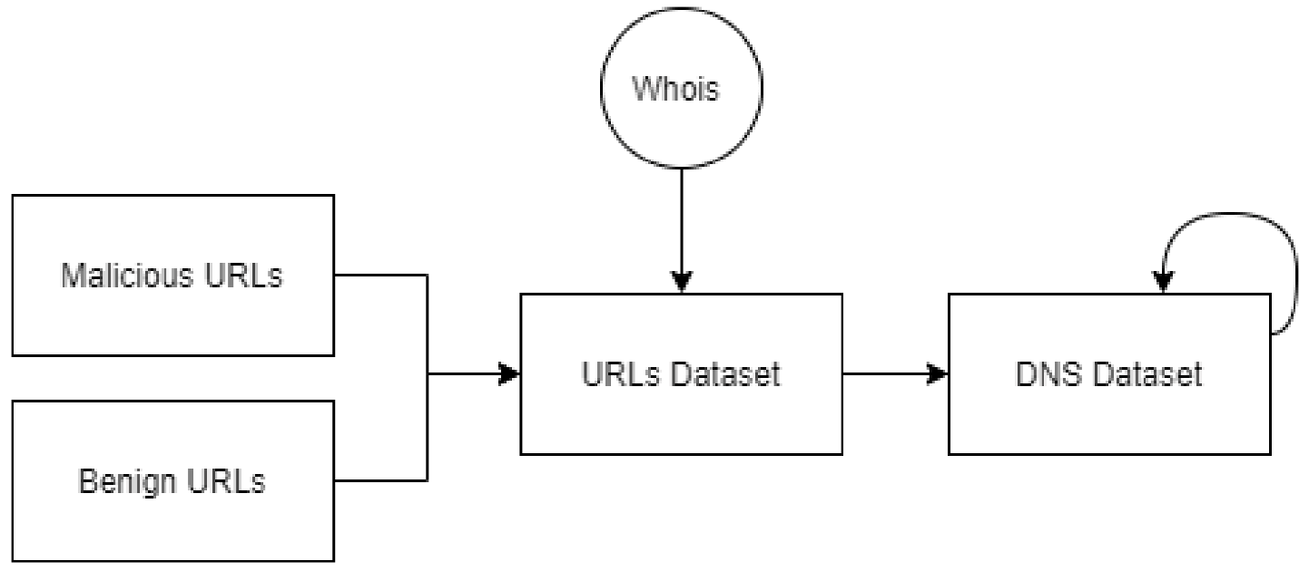
3.1. Data Collection

The main ingredient of ML models is the data on which the models are trained. Data collection should be as heterogeneous as possible to model reality. The data collected for this work include both malicious and benign URLs: the benign URLs are based on the Alexa top 1 million [62], and the malicious domains were crawled from multiple sources [63,64] to allow diversity and due to the fact they are fairly rare.

According to [65], 25% of all URLs in 2020 were malicious, suspicious, or moderately risky. Therefore, to make a realistic dataset, all the evaluations include all 1356 malicious active unique URLs, and consequently, 5345 benign active unique URLs as well. For each instance, the URL and domain information properties were crawled from Whois and their DNS records. Whois is a widely used Internet record listing that identifies who owns a domain, how to get in contact with them, the creation date, update dates, and expiration date of the domain. Whois records have been proven to be extremely useful and have developed into an essential resource for maintaining the integrity of the domain name registration and website ownership. Note that according to a study by ICANN (Internet Corporation for Assigned Names and Numbers) [66], many malicious attackers abuse the Whois system. Hence, only the information that could not be manipulated was used. A graphical representation of the data collection framework is illustrated in Figure 2.

Finally, based on these resources (Whois and DNS records), the following features were generated: the length of the domain, the number of consecutive characters, and the entropy of the domain from the URLs’ datasets. Next, the lifetime of the domain and the active time of domain were calculated from the Whois data. Based on the DNS response dataset (a total of 263,223 DNS records), the number of IP addresses, distinct geo-locations of the IP addresses, average Time to Live (TTL) value, and the Standard deviation of the TTL were extracted. For extracting the novel features (Section 3.5), Virus Total (VT) [67] and Urlscan [68] were used, where Urlscan was used to extract parameters such as the IP address of the page element of the URL.

3.2. Evaluation Metrics

Machine Learning (ML) is a subfield of computer science aimed at causing computers to act and improve over time autonomously by feeding them data in the form of observations and real-world interactions. In contrast to traditional programming, where input and algorithms are provided to receive an output, with ML, a list of inputs and their associated outputs are provided to extract the algorithm that maps the two.

ML algorithms are often categorized as either supervised or unsupervised. In supervised learning, each example is a pair consisting of an input vector (also called data point) and the desired output value (class/label). Unsupervised learning learns from data that have not been labeled, classified, or categorized. Instead of responding to feedback, unsupervised learning identifies commonalities in the data and reacts based on the presence or absence of such commonalities in each new piece of data.

In order to evaluate how a supervised model is adapted to a problem, the dataset needs to be split into two, namely, a training set and testing set. The training set is used to train the model, and the testing set is used to evaluate how well the model “learned” (i.e., by comparing the model predictions with the known labels). Usually, the train/test distribution is around 75%/25% (depending on the problem and the amount of data). Standard evaluation criteria are as follows: recall, precision, accuracy, F1-score, and loss. All of these criteria can easily be extracted from the evaluation’s confusion matrix.

A confusion matrix (

Table 1. Confusion matrix.

		Prediction Outcome
		Positive	Negative	Total
Actual Value	Positive	True Positive	False Negative	TP + FN
	Negative	False Positive	True Negative	FP + TN
	Total	P	N

) is commonly used to describe the performance of a classification model. Recall (Equation (2)) is defined as the number of correctly classified malicious examples out of all the malicious ones. Similarly, precision (Equation (3)) is the number of correctly classified malicious examples from all examples classified as malicious (both correctly and wrongly classified). Accuracy (Equation (1)) is used as a statistical measure of how well a classification test correctly identifies or excludes a condition. That is, the accuracy is the proportion of true results (both true positives and true negatives) among the total number of cases examined. Finally, the F1-score (Equation (4)) is a measure of a test’s accuracy. It considers both the precision and the recall of the test to compute the score. The F1-score is the harmonic average of the precision and recall, where an F1-score reaches its best value at 1 (perfect precision and recall) and worst at 0. These criteria are used as the main evaluation metric.

The problem of identifying malicious web domains is a supervised classification problem, as the correct label (i.e., malicious or benign) can be extracted using a blacklist-based method, as we describe in the next section.

$$Accuracy=\frac{TP+TN}{TP+FP+TN+FN}=\frac{T}{P+N}$$

(1)

$$Recall=\frac{TP}{TP+FN}$$

(2)

$$Precision=\frac{TP}{TP+FP}=\frac{TP}{P}$$

(3)

$$F_1-score=2·\frac{Precision·Recall}{Precision+Recall}$$

(4)

3.3. Feature Engineering

Based on the previous works surveyed, a set of features that are commonly used for malicious domain classification [11,13,22,23,27,28,35,69,70] were extracted. Specifically, the following nine features were used as the baseline (note that the focus of this work is on the potential use of robust features and not on the specific features; thus, WLOG, we evaluated a set of nine commonly used features):

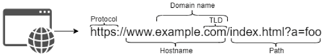
• Length of domain: The length of a domain is calculated by the domain name followed by the TLD (gTLD or ccTLD). Hence, the minimum length of a domain is four since the domain name needs to be at least one character (most domain names have at least three characters), and the TLD (gTLD or ccTLD) is composed of at least three characters (including the dot character) as well. For example, for the URL http://www.ariel-cyber.co.il; accessed on 20 March 2022, the length of the domain is 17 (the number of characters for the domain name—”ariel-cyber.co.il”).
• Number of consecutive characters: This is the maximum number of consecutive repeated characters in the domain. This includes the domain name and the TLD (gTLD or ccTLD). For example, for the domain “caabbbccccd.com” the maximum number of consecutive repeated characters value is 4, due to the four consecutive “c” characters.
• Entropy of the domain: The entropy of a domain is defined as: $-{\sum }_{j=1}^{n_i}\frac{count\left(c_j^i\right)}{length\left(Domai{n}_{\left(i\right)}\right)}·{log}_2\frac{count\left(c_j^i\right)}{length\left(Domai{n}_{\left(i\right)}\right)}$, where each $Domai{n}_{\left(i\right)}$ consists of $n_i$ distinct characters $\{c_1^i,c_2^i,\cdots ,c_{n_i}^i\}$. For example, for the domain “google.com”, the entropy is $-(5·(\frac{1}{10}·{log}_2\frac{1}{10})+2·(\frac{2}{10}·{log}_2\frac{2}{10})+3(·\frac{3}{10}·{log}_2\frac{3}{10}))=1.25$ The domain has 5 characters that appear once (“l”, “e”, “.”, “c”, and “m”), one character that appears twice (“g”) and one character that appears three times (“o”).
• Number of IP addresses: This is the number of distinct IP addresses in the domain’s DNS record. For example, for the list [“1.1.1.1”, “1.1.1.1”, and ”2.2.2.2”], the number of distinct IP addresses is 2.
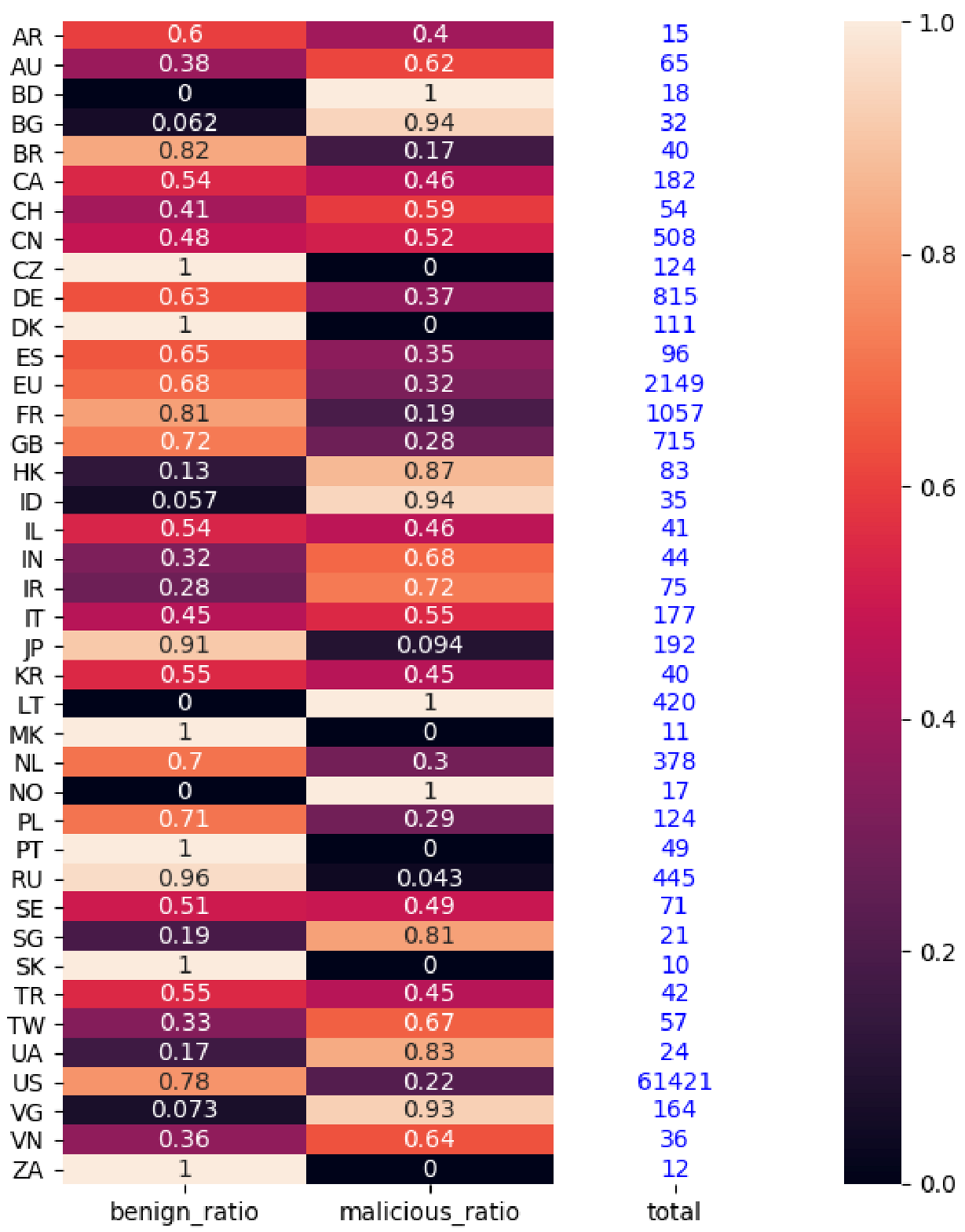
• Distinct geo-locations of the IP addresses: For each IP address in the DNS record, the countries for each IP were listed and the number of different countries was counted. For example, for the list of IP addresses [“1.1.1.1”, “1.1.1.1”, and ”2.2.2.2”] the list of countries is [“Australia”, “Australia”, and “France”] and the number of distinct countries is 2. Note that this feature relates to the number of different countries and not the country itself.
• Mean TTL value: For all the DNS records of the domain in the DNS dataset, the TTL values were averaged. For example, if a domain’s DNS records were checked 30 times, and in 20 of them the TTL value was “60” and in 10 the TTL value was “1200”, the mean is $\frac{20·60+10·1200}{30}=440$.
• Standard deviation of the TTL: The standard deviations of the TTL values for all the DNS records of the domain in the DNS dataset were calculated. For the “Mean TTL value” example above, the standard deviation of the TTL values is $537.401$.
• Lifetime of domain: This is the interval between a domain’s expiration date and creation date in years. For example, the domain “ariel-cyber.co.il”, according to Whois information, which was updated on 4 June 2018, was created on 14 May 2015 and expires on 14 May 2022. Therefore, the lifetime of the domain is the number of years from 14 May 2015 to 14 May 2022, i.e., 8.
• Active time of domain: Similar to the lifetime of a domain, the active time of a domain is calculated as the interval between a domain’s updated date and creation date in years. Using the same example as in the “Lifetime of domain”, the active time of the “ariel-cyber.co.il” domain is the number of years between 14 May 2015 and 14 May 2021, i.e., 6.

3.4. Robust Feature Selection

Next, the robustness of the set of features described above was evaluated to filter those that could significantly harm the classification process due to the adversary’s manipulations.

Table 2. Classic features and statistical properties (*—robust features).

Feature	Benign Mean (std)	Malicious Mean (std)
Length of domain	14.38 (4.06)	15.54 (4.09)
Number of consecutive characters *	1.29 (0.46)	1.46 (0.5)
Entropy of the domain	4.85 (1.18)	5.16 (1.34)
Number of IP addresses	2.09 (1.25)	1.94 (0.94)
Distinct geo-locations of the IP
addresses	1.00 (0.17)	1.02 (0.31)
Mean TTL value *	7578.13 (17,781.47)	8039.92 (15,466.29)
Standard deviation of the TTL	2971.65 (8777.26)	2531.38 (7456.62)
Lifetime of domain *	10.98 (7.46)	6.75 (5.77)
Active time of domain *	8.40 (6.79)	4.64 (5.66)

lists the common features along with the mean value and standard deviation (note that the std in some cases (e.g., mean TTL value) is higher due to fact that these features have a positive value by definition.) For malicious and benign URLs based on our dataset, note that some features have similar mean values for both benign and malicious instances while they are commonly used. Furthermore, whereas “Standard deviation of the TTL” has distinct values for benign and malicious domains, we later show that an intelligent adversary can easily manipulate this feature, leading to a benign classification of malicious domains.

In order to understand the malicious abilities of an adversary, the base features were manipulated over a wide range of possible values, one feature at a time. This analysis considers an intelligent adversary with black-box access to the model (i.e., a set of features or output for a given input). The robustness analysis is based on an ANN model that classifies the manipulated samples, where the train set is the empirically crawled data, and the test set includes the manipulated malicious samples. Figure 3 depicts the possible adversary manipulations over any of the features. We chose recall for the evaluation metric, representing the average detection rate after modifications.

The well-known features were divided into three groups: robust features, robust features that seemed non-robust (defined as semi-robust), and non-robust features. Next, it it is shown how an attacker can manipulate the classifier for each feature and define its robustness:

1.

“Length of domain”: an adversary can easily purchase a short or long domain to result in a benign classification for a malicious domain; hence, this feature was classified as non-robust.

2.

“Number of consecutive characters”: as depicted in Figure 3, manipulating the “Number of consecutive characters” feature can significantly lower the prediction percentage (e.g., move from three consecutive characters to one or two). Still, as depicted in Table 2, on average, there were 1.46 consecutive characters in malicious domains (with a low standard deviation). Therefore, as this feature’s minimal value is 1, it is considered to be a robust feature.

3.

“Entropy of the domain”: in order to manipulate the “Entropy of the domain” feature as a benign domain entropy, the adversary can create a domain name with an entropy of less than 4. For example, the domain “ddcd.cc” is available for purchase. The entropy for this domain is $1.44$. This value falls precisely in the entropy area of the benign domains defined by the trained model. This example breaks the model and causes a malicious domain to look like a benign URL. Hence, this feature was classified as non-robust.

4.

“Number of IP addresses”: note that an adversary can add many A records to the DNS zone file of its domain to imitate a benign domain. Thus, to manipulate the number of IP addresses, an intelligent adversary only needs to have several different IP addresses and add them to the zone file. This fact causes this feature to be classified as non-robust.

5.

“Distinct Geo-locations of the IP addresses”: in order to be able to circumvent the model with the “Distinct Geolocations of the IP addresses” feature, the adversary needs to use several IP addresses from different geo-locations. Suppose the adversary can determine how many different countries are sufficient to mimic the number of distinct countries of benign domains. In that case, he will be able to append this number of IP addresses (a different IP address from each geo-location) in the DNS zone file. Moreover, because this feature counts the number of the countries, the attacker can choose a set of countries to meet the desired number. Thus, this feature was also classified as non-robust (this assumption gave us the motivation for one of our novel features which is based on the rank of the countries and not only the number of the countries).

6.

“Mean TTL value” and “Standard deviation of the TTL”: there is a clear correlation between the “Mean TTL value” and the “Standard deviation of the TTL” features since the value manipulated by the adversary is the TTL itself. Thus, it makes no difference if the adversary cannot manipulate the “Mean TTL value” feature if the model uses both. In order to robustify the model, it is better to use the “Mean TTL value” feature without the “Standard deviation of the TTL”. Solely in terms of the “Mean TTL value” feature, Figure 3 shows that manipulation will not result in a false classification since the prediction percentage does not drop dramatically, even when this feature is drastically manipulated. Therefore, this feature (“Mean TTL value”) is considered to be robust.

An adversary can set the DNS TTL values to [0,120,000] (according to the RFC 2181 [71] the TTL value range is from 0 to $2^{31}-1$). Figure 3 shows that even manipulating the value of this feature to 60,000 will deceive the model and cause a malicious domain to be wrongly classified as a benign URL. Therefore, the “Standard deviation of the TTL” is considered a non-robust feature.

7.

“Lifetime of domain”: As for the lifetime of domains, based on Shi et al.  [23], we know that a benign domain’s lifetime is typically much longer than a malicious domain’s lifetime. In order to deceive the model by manipulating the “Lifetime of domain” feature, the adversary must buy an old domain that is available on the market. Even though it is possible to buy an appropriate domain, it is expensive (if feasible). Hence, we considered this to be a robust feature.

8.

“Active time of domain”: Similar to the previous feature, in order to overcome the “Active time of domain” feature, an adversary has to find a domain with a particular active time, which is much more tricky. It is complex, expensive, and perhaps unfeasible. Therefore we considered it to be a robust feature.

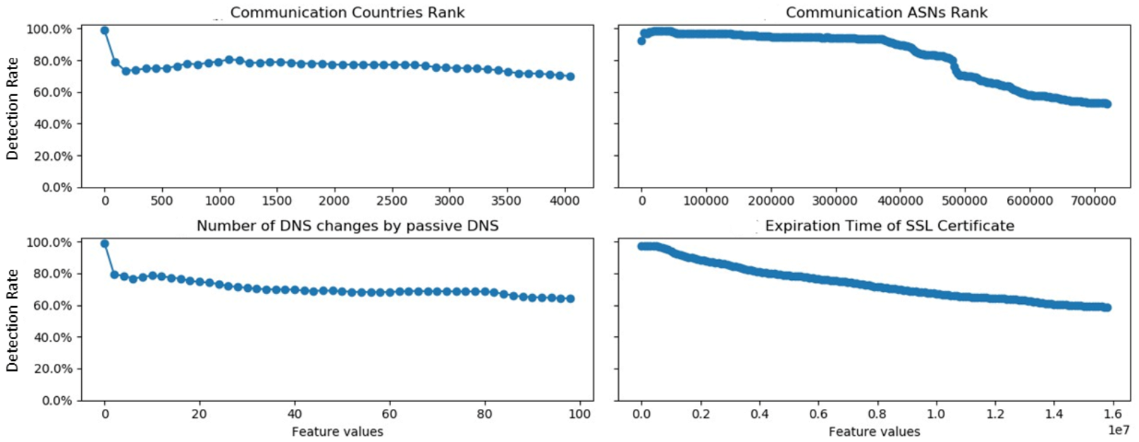
Based on the analysis above, the robust features presented in Table 2 were selected, and the non-robust ones were dropped. Using this subset, the model was trained and achieved an accuracy of 95.71% with an F1-score of 88.78%, compared to an accuracy of 97.2% and an F1-score of 90.23% when using all the features (i.e., including the robust ones). Therefore, we extended our analysis and searched for new features that would meet the robustness requirements to build a robust model with a higher F1-score.

3.5. Novel Features

We aim to validate that manipulating the features in order to result in the misclassification of malicious instances will require a disproportionate effort that will deter the attacker from doing so. The four novel features were designed according to this paradigm based on two communication information properties, passive DNS changes, and the expiration time of the SSL certificate. For each IP, we used Urlscan [68] to extract the geo-location, which in turn was appended to a communication country list. The communication Autonomous System Numbers (ASNs) is a list of ASNs, extracted using Urlscan, each IP address, and appended the ASNs list. Benign-malicious ratio tables for communication countries, and communication ASNs (Figure 4 and Figure 5) were created using the URL dataset and the Urlscan service. The ratio tables were calculated for each element E (country—for the communication countries ratio table; ASN—for the communication ASNs ratio table). Each table represents the probability that a URL associated with a country (ASN) is malicious. In order to extract the probabilities, the number of malicious URLs associated with E was divided by the total URLs associated with E. Initially, due to the heterogeneity of the dataset (i.e., there exist some elements that appear only a few times), the ratio tables appeared to be biased. To overcome this challenge, an initial threshold was set as an insertion criterion which is later detailed in Algorithm 1.

The following is a detailed summary of the novel features:

• Communication Countries Rank (CCR): This feature looks at the communication countries with respect to the communication IPs, and uses the countries ratio table to rank a specific URL. The motivation is to gain a broader perspective.
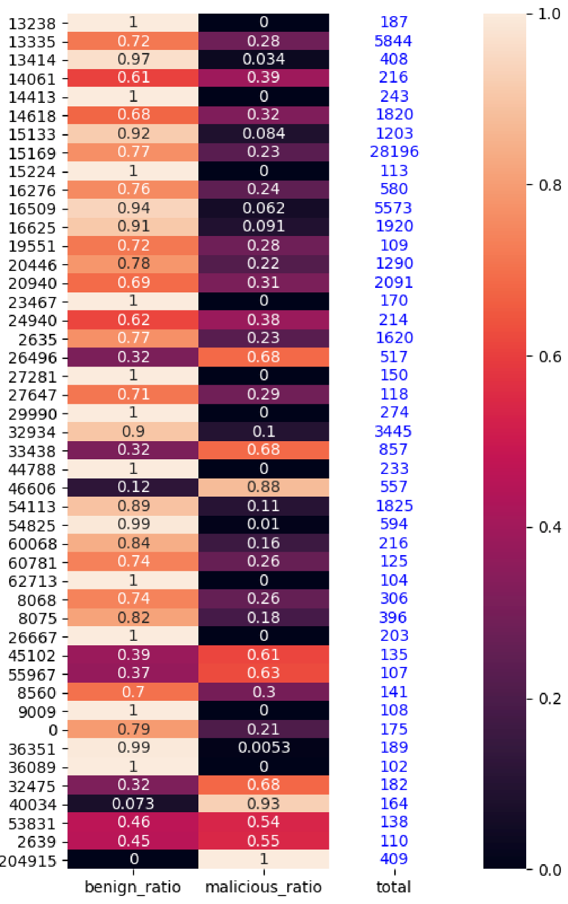
• Communication ASNs Rank (CAR): Similarly, this feature analyzes the communication ASNs with respect to the communication IPs, and uses the ASNs ratio table to rank a specific URL. While there is some correlation between the ASNs and the countries, the second feature examines each Autonomous System (AS) within each country to gain a broader perspective.
• Number of passive DNS changes: When inspecting the passive DNS records, benign domains emerged as having much more significant DNS changes that the sensors (of the company that collects the DNS records) could identify, unlike malicious domains (i.e., 26.4 vs. 8.01, as reported in

  Table 3. Novel features and statistical properties.

  Feature	Benign Mean (std)	Malicious Mean (std)
  Communication Countries Rank (CCR)	31.31 (91.16)	59.40 (215.15)
  Communication ASNs Rank (CAR)	935.59 (12,258.99)	12,979.38 (46,384.86)
  Number of passive DNS changes	26.40 (111.99)	8.01 (16.63)
  Expiration time of SSL certificate	$1.547\times {10}^7$ ($2.304\times {10}^7$)	$4.365\times {10}^6$ ($1.545\times {10}^7$)

  ). The number of DNS record changes was counted for the “Number of passive DNS changes”, which is somewhat similar to other features described in other works [11,25]. Nonetheless, these features require much more elaborated information, which is not publicly available. On the other hand, this feature can be extracted from passive DNS records obtained from VirusTotal, which are scarce (in terms of record types).
• Expiration time of SSL certificate: When installing an SSL certificate, a Certificate Authority (CA) conducts a validation process. Depending on the type of certificate, the CA verifies the organization’s identity before issuing the certificate. When analyzing our data, it was noted that most malicious domains do not use valid SSL certificates and those that only use one for a short period. Therefore, this feature was engineered in order to represent the time the SSL certificate remains valid. The “Expiration time of SSL certificate”, in contrast to the binary feature version used by Ranganayakulu et al. [69], extends the scope and represents both the existence of an SSL certificate and the remaining time until the SSL certificate expires.

Algorithm 1 Communication Rank

Input: URL, Threshold, Type Output: Rank (CCR or CAR) if Type = Countries then    ItemsList = communication countries list of the URL else    ItemsList = ASNs list of the URL end if $Rank=0$ for$Item$ in $ItemsList$ do    $Ratio=0.75$ Init value    $Total\_norm=1$ Init value    if $TotalOccurrences\left(Item\right)>=Threshold$ then      $Total\_norm=Normalize\left(Item\right)$      $Ratio=BenignRatio\left(Item\right)$    end if    $Rank+=({log}_{0.5}(Ratio+ϵ)/Total\_norm)$ end for

Algorithm 1 receives a URL as an input and returns its communication country rate or the ASN communication rate (based on the type of the input in the algorithm). For each item (i.e., country or ASN), first the algorithm initializes the value of the ratio variable to 0.75 (according to [65], 25% of all URLs in 2020 were malicious, suspicious, or moderately risky). It then normalizes an item’s total occurrences (Total_norm) to be 1. Next, in Step 9, if an item’s total number of occurrences is ≥ to the threshold, the algorithm replaces the ratio. It normalizes occurrences to the correct values according to the ratio tables given in Figure 4 and Figure 5. Finally, the algorithm sums the rank with a log base of 0.5 of the ratio ($ϵ$ is a very small value that was added for the special case where $Ratio=0$) and divides this value by the normalized total occurrences.

Figure 6 depicts the detection rate as a function of the novel features’ values for each feature in Table 3. This evaluation proves that manipulating our novel features does not affect the robust model (i.e., the detection rate remains steady). The negative correlation between “Expiration time of SSL certificate” feature and the detection rate may raise concern. Nevertheless, it is noteworthy that the average value for malicious domains is three times higher than the benign ones. While, theoretically, the adversary can lower this value, the implications of such an action mean acquiring (or attaining for free) an SSL certificate. Since there is a validation process involved in the acquisition of an SSL certificate, doing so will cause the adversary to lose its anonymity and disclose its identity.

4. Empirical Analysis and Evaluation

This section describes the testbed used to evaluate models based on the types of features (both robust and not). General settings are provided for each of the models (e.g., the division of the data into training and test sets), as well as the parameters used to configure each of the models, and the efficiency of each model. (our code is publicly available at https://github.com/nitayhas/robust-malicious-url-detection; accessed on 20 March 2022).

4.1. Experimental Design

In addition to intelligently choosing the model parameters, one should verify that the data used for the learning phase accurately represent the domain malware’s real-world distribution. Hence, the dataset was constructed such that 75% were benign domains, and the remaining 25% were malicious domains (~5000 benign URLs and ~1350 malicious domains, respectively) [65].

There are many ways to define the efficiency of a model. A broad set of metrics was extracted to account for most of them, including accuracy, recall, F1-score, and training time. Note that for each model, the dataset was split into train and test sets where 75% of the data (both benign and malicious) were assigned to the train set, and the remaining domains were assigned to the test set. Note that the entire dataset included 75% benign samples. Later, when we trained a model, we used 75% of the dataset for the training process and 25% for the evaluation (i.e., test set).

The evaluation measured the efficiency of the different models while varying the robustness of the features included in the model. Specifically, four classical models (i.e., Logistic Regression, SVM, ELM, and ANN) were trained using the following feature sets:

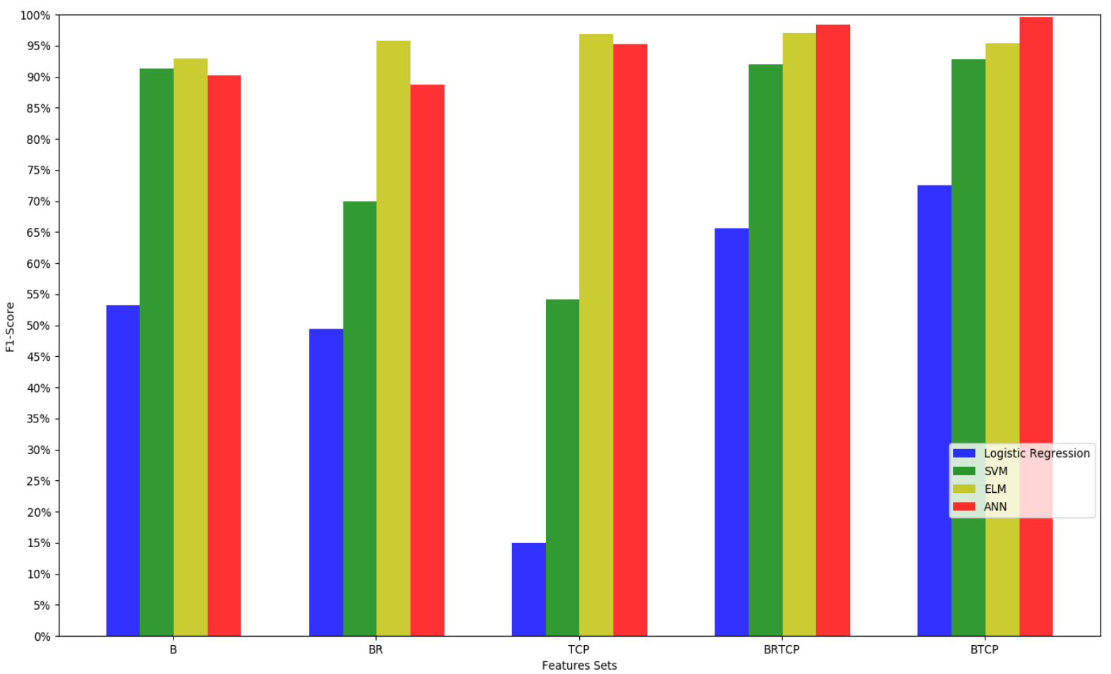
• Base (B)—the set of commonly used features in previous works (see Table 2 for more details).
• Base Robust (BR)—the subset of robust base features (marked with a * in Figure 3).
• “TCP” (TCP)—the four novel features: Time of SSL certificate, Communication ranks (CCR and CAR) and PassiveDNS changes (see Table 3).
• Base Robust + “TCP” (BRTCP)—the combination (union) of BR and TCP, the robust subset of all features.
• Base + “TCP” (BTCP)—the union of B and TCP.

4.2. Experimental Results

Four commonly used classification models were considered: Logistic Regression (LR), Support Vector Machines (SVM), Extreme Learning Machine (ELM), and Artificial Neural Networks (ANN). All the models were trained and evaluated on a Dell XPS 8920 computer, Windows 10 64Bit OS with 3.60GHz Intel Core i7-7700 CPU, 16GB of RAM, and NVIDIA GeForce GTX 1060 6GB. In the following paragraphs, we describe the experimental results for each model, followed by a short discussion of the findings and their implications.

4.2.1. Logistic Regression

As a baseline for the evaluation process, and before using the nonlinear models, the LR classification model was used. The LR model with the five feature sets (Base, Robust Base, TCP, BRTCP, BTCP) was trained.

Table 4. Model performance—logistic Regression.

Feature Set	Accuracy	Recall	F1-Score
Base	89.99%	38.82%	53.21%
Robust Base	88.33%	38.87%	49.42%
TCP	86.20%	8.30%	14.99%
BRTCP	88.82%	52.46%	65.57%
BTCP	92.86%	64.14%	72.48%

shows that the different feature sets resulted in similar accuracy rates. However, the accuracy rate measures how well the model predicts (i.e., TP + TN)with respect to all the predictions (i.e., TP + TN + FP + FN). Thus, given the unbalanced dataset (75% of the dataset are benign and 25% are malicious domains), ~90% accuracy is not necessarily a sufficient result for malware detection. For example, the TCP feature set has high accuracy and, at the same time, a very poor F1-Score, due to the high precision rate and poor recall rate. As the recall is low for all features sets, the accuracy rate is not a good measure in this domain. Consequently, we focused on the F1-score measure, the harmonic mean of the precision, and the recall measures.

4.2.2. Support Vector Machine (SVM)

Compared to the results of the LR model (Table 4), the results of the SVM model (

Table 5. Model performance—SVM.

Feature Set	Accuracy	Recall	F1-Score
Base	96.49%	91.20%	91.36%
Robust Base	90.14%	56.51%	69.93%
TCP	83.10%	60.21%	54.21%
BRTCP	96.78%	91.37%	92.02%
BTCP	97.95%	90.73%	92.83%

) show a significant improvement in the recall and F1-score measures; e.g., for Base, the recall and the F1-score measures were both above 90%. It should be noted that the model that trained on the Base feature set resulted in a higher recall (and F1-score) compared to the one trained on the Robust Base feature set. Nonetheless, it is also noteworthy that the Robust Base feature set is robust to adversarial manipulation and uses less than half of the features provided in the training phase with the Base feature set. This discussion also applies to the BRTCP and BTCP feature sets. Another advantage of including the novel features is that models converge much faster. The results are based on the analysis of a non-manipulated dataset. As stated above, the Base feature set includes some non-robust features. Hence, an intelligent adversary can manipulate the values of these features, resulting in the wrong classification of malicious instances (to the extreme of $0\%$ recall). However, an intelligent adversary will need to invest much more effort with a model that was trained using the Robust Base or TCP features since each was specifically chosen to avoid such manipulations. In order to find models that were also efficient on the non-manipulated dataset, the two sophisticated models were examined in the analysis, the ELM model Shi et al. [23] provided and the ANN model.

4.2.3. ELM

The architecture of the ELM is the one previously used [23]: one input layer, one hidden layer, and one output layer. Activation function: first layer—ReLU; hidden layer—Sigmoid. Overall, the ELM model resulted (see

Table 6. Model performance—ELM.

Feature Set	Accuracy	Recall	F1-Score
Base	98.17%	88.81%	92.92%
Robust Base	98.83%	92.24%	95.81%
TCP	98.88%	94.64%	96.84%
BRTCP	98.86%	95.82%	97.07%
BTCP	98.19%	93.09%	95.34%

) in a high accuracy and higher recall rates compared to Table 4, for any feature set. When compared to the SVM models, the Base model resulted in a lower recall rate (though a higher F1-score was achieved with the ELM model). On the other hand, the Robust Base resulted in a higher recall rate with the ELM model compared to the SVM model. Even though the Robust Base feature set had a low dimensional space, the three rates (i.e., accuracy, recall, and F1-score) were higher than those of the Base feature set. Using the sets that include the novel features increased these metrics while improving the robustness of the model at the same time.

4.2.4. ANN

The architecture of the neural network was as follows: one input layer, three hidden layers, and one output layer. Activation function: first layer—ReLU; first hidden layer—RELU; second hidden layer—LeakyReLU; third hidden layer—Sigmoid. Batch size: −150, with a learning rate of 0.01; solver: Adam with ${\beta }_1$ = 0.9 and ${\beta }_2=0.999$. Similar to the ELM results, the ANN results (

Table 7. Model performance—ANN.

Feature Set	Accuracy	Recall	F1-Score
Base	97.20%	88.03%	90.23%
Robust Base	95.71%	83.63%	88.78%
TCP	98.03%	96.83%	95.24%
BRTCP	99.36%	98.77%	98.42%
BTCP	99.82%	99.47%	99.56%

) show high performance with all feature sets. For the “basic” feature sets (i.e., Base and Robust Base), the ELM models resulted in higher recall and F1-score. Nevertheless, the main focus was in the BTCP feature set and, more specifically, on the BRTCP variant, where the ANN models resulted in a higher recall and F1-score.

Our analysis concludes with Figure 7, which depicts the F1-scores of the feature sets for all the models.

All the results provided in this article are based on clean data (i.e., with no adversarial manipulation). Naturally, given an adversarial environment where the attacker can manipulate the values of the features, models which are based on the Robust Base or TCP feature sets will dominate models that are trained using the Base dataset. Thus, by showing that the Robust Base feature set does not dramatically decrease the performance of the classifier using clean data and that adding the novel feature improves the model’s performance as well as its robustness, it leads to the conclusion that malicious domain classifiers should use this feature set for robust malicious domain detection.

5. Conclusions

Numerous attempts have been made to tackle the problem of identifying malicious domains. However, many fail to successfully classify malware in realistic environments where an adversary can manipulate the features in order to make the model wrongly classify malicious domains. Specifically, this research used a large empirical dataset that was crawled over a significant amount of time at different hours of the day, and captures traffic generated in various countries and continents. Based on this rich dataset, this paper tackled the case where an attacker has access to the model (i.e., a set of features or output for a given input) and tampers with the domain properties. This tampering has a catastrophic effect on the model’s efficiency. As a countermeasure, we propose two feature-based mechanisms: (I) an intelligent feature selection procedure that is robust to adversarial manipulation. We evaluated the robustness of each feature, taking into account both the hardness of changing its value and the effects of such manipulations on the classifier; (II) a novel and robust feature engineering process. Based on the domains’ properties, we engineered a set of four features which are robust to adversarial manipulation and, together with the common features, improve the classifiers’ performance.

We empirically evaluated the common feature set as well as our novel ones using a large dataset, which took into account both malicious and benign models. To extend our evaluation, we picked a broad set of well-known machine learning algorithms. Our evaluation showed that models trained using the robust features are more precise in terms of manipulated data while maintaining good results on clean data as well.

From the industry perspective, our solution can be easily adopted either in any organization’s DPI center solution, Firewall, Load Balancer, behavioral analytic or as a client agent that will query a cloud-service dataset. Further research is needed to create models that classify malicious domains into malicious attack types, either in terms of a more extensive list of models or by sampling data in a stratified way, validating the amount of data for any feature value. Another promising direction would be to cluster a set of malicious domains into one cyber campaign.

References

1. Vincent, N.E.; Pinsker, R. IT risk management: Interrelationships based on strategy implementation. Int. J. Account. Inf. Manag. 2020, 28, 553–575. [Google Scholar] [CrossRef]
2. Blum, A.; Wardman, B.; Solorio, T.; Warner, G. Lexical feature based phishing URL detection using online learning. In Proceedings of the Workshop on Artificial Intelligence and Security, Krakow, Poland, 15–18 February 2010; pp. 54–60. [Google Scholar]
3. Khonji, M.; Iraqi, Y.; Jones, A. Phishing detection: A literature survey. IEEE Commun. Surv. Tutor. 2013, 15, 2091–2121. [Google Scholar] [CrossRef]
4. Le, A.; Markopoulou, A.; Faloutsos, M. Phishdef: Url Names Say It All. In Proceedings of the 2011 IEEE INFOCOM, Shanghai, China, 10–15 April 2011; pp. 191–195. [Google Scholar]
5. Prakash, P.; Kumar, M.; Kompella, R.R.; Gupta, M. Phishnet: Predictive Blacklisting to Detect Phishing Attacks. In Proceedings of the 2010 IEEE INFOCOM, San Diego, CA, USA, 14–19 March 2010; pp. 1–5. [Google Scholar]
6. Sheng, S.; Wardman, B.; Warner, G.; Cranor, L.F.; Hong, J.; Zhang, C. An empirical analysis of phishing blacklists. In Proceedings of the Conference on Email and Anti-Spam, Mountain View, CA, USA, 16–17 July 2009. [Google Scholar]
7. Sandell, N.; Varaiya, P.; Athans, M.; Safonov, M. Survey of decentralized control methods for large scale systems. IEEE Trans. Autom. Control 1978, 23, 108–128. [Google Scholar] [CrossRef]
8. Canali, D.; Cova, M.; Vigna, G.; Kruegel, C. Prophiler: A fast filter for the large-scale detection of malicious web pages. In Proceedings of the International Conference on World Wide Web, Hyderabad, India, 28 March–1 April 2011; pp. 197–206. [Google Scholar]
9. Hason, N.; Dvir, A.; Hajaj, C. Robust Malicious Domain Detection. In Cyber Security Cryptography and Machine Learning; Dolev, S., Kolesnikov, V., Lodha, S., Weiss, G., Eds.; Springer: Cham, Switzerland, 2020; pp. 45–61. [Google Scholar]
10. Ahmed, M.; Khan, A.; Saleem, O.; Haris, M. A Fault Tolerant Approach for Malicious URL Filtering. In Proceedings of the International Symposium on Networks, Computers and Communications, Rome, Italy, 19–21 June 2018; pp. 1–6. [Google Scholar]
11. Antonakakis, M.; Perdisci, R.; Dagon, D.; Lee, W.; Feamster, N. Building a Dynamic Reputation System for DNS. In Proceedings of the 19th USENIX conference on Security, Washington, DC, USA, 11–13 August 2010; pp. 273–290. [Google Scholar]
12. Berger, H.; Dvir, A.Z.; Geva, M. A wrinkle in time: A case study in DNS poisoning. Int. J. Inf. Secur. 2021, 20, 313–329. [Google Scholar] [CrossRef]
13. Bilge, L.; Sen, S.; Balzarotti, D.; Kirda, E.; Kruegel, C. Exposure: A Passive DNS Analysis Service to Detect and Report Malicious Domains. Trans. Inf. Syst. Secur. 2014, 16, 1–28. [Google Scholar] [CrossRef]
14. Caglayan, A.; Toothaker, M.; Drapeau, D.; Burke, D.; Eaton, G. Real-time detection of fast flux service networks. In Proceedings of the Conference For Homeland Security, Cybersecurity Applications and Technology, Washington, DC, USA, 3–4 March 2009; pp. 285–292. [Google Scholar]
15. Choi, H.; Zhu, B.B.; Lee, H. Detecting Malicious Web Links and Identifying Their Attack Types. WebApps 2011, 11, 218. [Google Scholar]
16. Dolberg, L.; François, J.; Engel, T. Efficient Multidimensional Aggregation for Large Scale Monitoring. In Proceedings of the 26th Large Installation System Administration Conference, Washington, DC, USA, 3–8 November 2013; pp. 163–180. [Google Scholar]
17. Harel, N.; Dvir, A.; Dubin, R.; Barkan, R.; Shalala, R.; Hadar, O. MiSAL-A minimal quality representation switch logic for adaptive streaming. Multimed. Tools Appl. 2019, 78, 1–26. [Google Scholar]
18. Hu, Z.; Chiong, R.; Pranata, I.; Susilo, W.; Bao, Y. Identifying malicious web domains using machine learning techniques with online credibility and performance data. In Proceedings of the Congress on Evolutionary Computation (CEC), Vancouver, BC, Canada, 24–29 July 2016; pp. 5186–5194. [Google Scholar]
19. Huang, G.B.; Zhu, Q.Y.; Siew, C.K. Extreme learning machine: Theory and applications. Neurocomputing 2006, 70, 489–501. [Google Scholar] [CrossRef]
20. Nelms, T.; Perdisci, R.; Ahamad, M. ExecScent: Mining for New C&C Domains in Live Networks with Adaptive Control Protocol Templates. In Proceedings of the 22nd USENIX Security Symposium, Washington, DC, USA, 14–16 August 2013; pp. 589–604. [Google Scholar]
21. Peng, T.; Harris, I.; Sawa, Y. Detecting phishing attacks using natural language processing and machine learning. In Proceedings of the International Conference on Semantic Computing, Laguna Hills, CA, USA, 31 January–2 Februay 2018; pp. 300–301. [Google Scholar]
22. Rahbarinia, B.; Perdisci, R.; Antonakakis, M. Efficient and accurate behavior-based tracking of malware-control domains in large ISP networks. ACM Trans. Priv. Secur. 2016, 19, 4. [Google Scholar] [CrossRef]
23. Shi, Y.; Chen, G.; Li, J. Malicious Domain Name Detection Based on Extreme Machine Learning. Neural Process. Lett. 2017, 48, 1–11. [Google Scholar] [CrossRef]
24. Sun, X.; Tong, M.; Yang, J.; Xinran, L.; Heng, L. HinDom: A Robust Malicious Domain Detection System based on Heterogeneous Information Network with Transductive Classification. In Proceedings of the International Symposium on Research in Attacks, Intrusions and Defenses, Beijing, China, 23–25 September 2019; pp. 399–412. [Google Scholar]
25. Torabi, S.; Boukhtouta, A.; Assi, C.; Debbabi, M. Detecting Internet Abuse by Analyzing Passive DNS Traffic: A Survey of Implemented Systems. Commun. Surv. Tutor. 2018, 20, 3389–3415. [Google Scholar] [CrossRef]
26. Yadav, S.; Reddy, A.K.K.; Reddy, A.L.N.; Ranjan, S. Detecting Algorithmically Generated Domain-flux Attacks with DNS Traffic Analysis. Trans. Netw. 2012, 20, 1663–1677. [Google Scholar] [CrossRef]
27. Antonakakis, M.; Perdisci, R.; Lee, W.; Vasiloglou, N.; Dagon, D. Detecting Malware Domains at the Upper DNS Hierarchy. In Proceedings of the 20th USENIX Security Symposium, San Francisco, CA, USA, 8–12 August 2011; Volume 11, pp. 1–16. [Google Scholar]
28. Perdisci, R.; Corona, I.; Giacinto, G. Early detection of malicious flux networks via large-scale passive DNS traffic analysis. IEEE Trans. Dependable Secur. Comput. 2012, 9, 714–726. [Google Scholar] [CrossRef]
29. Papernot, N.; McDaniel, P.; Wu, X.; Jha, S. Distillation as a Defense to Adversarial Perturbations against Deep Neural Networks. In Proceedings of the IEEE Symposium on Security and Privacy, San Jose, CA, USA, 22–26 May 2016. [Google Scholar]
30. Tong, L.; Li, B.; Hajaj, C.; Xiao, C.; Zhang, N.; Vorobeychik, Y. Improving Robustness of ML Classifiers against Realizable Evasion Attacks Using Conserved Features. In Proceedings of the 28th USENIX Security Symposium, Santa Clara, CA, USA, 14–16 August 2019. [Google Scholar]
31. Jung, J.; Sit, E. An empirical study of spam traffic and the use of DNS black lists. In Proceedings of the SIGCOMM Conference on Internet Measurement, Taormina Sicily, Italy, 25–27 October 2004; pp. 370–375. [Google Scholar]
32. Mishsky, I.; Gal-Oz, N.; Gudes, E. A topology based flow model for computing domain reputation. In Proceedings of the IFIP Annual Conference on Data and Applications Security and Privacy, Fairfax, VA, USA, 13–15 July 2015; pp. 277–292. [Google Scholar]
33. Othman, H.; Gudes, E.; Gal-Oz, N. Advanced Flow Models for Computing the Reputation of Internet Domains. In Proceedings of the IFIP International Conference on Trust Management, Toronto, ON, Canada, 9–13 July 2017; pp. 119–134. [Google Scholar]
34. Dey, S.; Jain, E.; Das, A. Machine Learning Features for Malicious URL Filtering—The Survey. arXiv 2019, arXiv:2019.0621. [Google Scholar]
35. Sahoo, D.; Liu, C.; Hoi, S.C. Malicious URL detection using machine learning: A survey. arXiv 2017, arXiv:1701.07179. [Google Scholar]
36. Shahzad, H.; Sattar, A.R.; Skandaraniyam, J. From Real Malicious Domains to Possible False Positives in DGA Domain Detection. In Proceedings of the 2021 IEEE 13th International Conference on Computer Research and Development (ICCRD), Beijing, China, 5–7 January 2021; pp. 6–10. [Google Scholar] [CrossRef]
37. Zhang, S.; Zhou, Z.; Li, D.; Zhong, Y.; Liu, Q.; Yang, W.; Li, S. Attributed Heterogeneous Graph Neural Network for Malicious Domain Detection. In Proceedings of the 2021 IEEE 24th International Conference on Computer Supported Cooperative Work in Design (CSCWD), Dalian, China, 5–7 May 2021; pp. 397–403. [Google Scholar] [CrossRef]
38. Iwahana, K.; Takemura, T.; Cheng, J.C.; Ashizawa, N.; Umeda, N.; Sato, K.; Kawakami, R.; Shimizu, R.; Chinen, Y.; Yanai, N. MADMAX: Browser-Based Malicious Domain Detection Through Extreme Learning Machine. IEEE Access 2021, 9, 78293–78314. [Google Scholar] [CrossRef]
39. Kumi, S.; Lim, C.; Lee, S.G. Malicious url detection based on associative classification. Entropy 2021, 23, 182. [Google Scholar] [CrossRef]
40. Janet, B.; Kumar, R.J.A. Malicious URL Detection: A Comparative Study. In Proceedings of the 2021 International Conference on Artificial Intelligence and Smart Systems (ICAIS), Coimbatore, India, 25–27 March 2021; pp. 1147–1151. [Google Scholar]
41. Srinivasan, S.; Vinayakumar, R.; Arunachalam, A.; Alazab, M.; Soman, K. DURLD: Malicious URL detection using deep learning-based character level representations. In Malware Analysis Using Artificial Intelligence and Deep Learning; Springer: Berlin/Heidelberg, Germany, 2021; pp. 535–554. [Google Scholar]
42. Cyprienna, R.A.; Zo Lalaina Yannick, R.; Randria, I.; Raft, R.N. URL Classification based on Active Learning Approach. In Proceedings of the 2021 3rd International Cyber Resilience Conference (CRC), Langkawi Island, Malaysia, 29–31 January 2021; pp. 1–6. [Google Scholar] [CrossRef]
43. Goodfellow, I.J.; Shlens, J.; Szegedy, C. Explaining and Harnessing Adversarial Examples; In Proceedings of the 3rd International Conference on Learning Representations, San Diego, CA, USA, 7–9 May 2015.
44. Nelson, B.; Barreno, M.; Chi, F.J.; Joseph, A.D.; Rubinstein, B.I.; Saini, U.; Sutton, C.A.; Tygar, J.D.; Xia, K. Exploiting Machine Learning to Subvert Your Spam Filter. LEET 2008, 8, 1–9. [Google Scholar]
45. Fogla, P.; Sharif, M.I.; Perdisci, R.; Kolesnikov, O.M.; Lee, W. Polymorphic Blending Attacks. In Proceedings of the 15th USENIX Security Symposium, Austin, TX, USA, 10–12 August 2006; pp. 241–256. [Google Scholar]
46. Newsome, J.; Karp, B.; Song, D. Paragraph: Thwarting signature learning by training maliciously. In Proceedings of the International Workshop on Recent Advances in Intrusion Detection, Hamburg, Germany, 20–22 September 2006; pp. 81–105. [Google Scholar]
47. Rodrigues, R.N.; Ling, L.L.; Govindaraju, V. Robustness of multimodal biometric fusion methods against spoof attacks. J. Vis. Lang. Comput. 2009, 20, 169–179. [Google Scholar] [CrossRef]
48. Madry, A.; Makelov, A.; Schmidt, L.; Tsipras, D.; Vladu, A. Towards Deep Learning Models Resistant to Adversarial Attacks. In Proceedings of the Sixth International Conference on Learning Representations, Vancouver, BC, Canada, 30 April–3 May 2018. [Google Scholar]
49. Raghunathan, A.; Steinhardt, J.; Liang, P. Certified Defenses against Adversarial Examples. In Proceedings of the Sixth International Conference on Learning Representations, Vancouver, BC, Canada, 30 April–3 May 2018. [Google Scholar]
50. Song, Y.; Kim, T.; Nowozin, S.; Ermon, S.; Kushman, N. Pixeldefend: Leveraging Generative Models to Understand and Defend against Adversarial Examples. In Proceedings of the Sixth International Conference on Learning Representations, Vancouver, BC, Canada, 30 April–3 May 2018. [Google Scholar]
51. Berger, H.; Hajaj, C.; Mariconti, E.; Dvir, A. Crystal Ball: From Innovative Attacks to Attack Effectiveness Classifier. IEEE Access 2022, 10, 1317–1333. [Google Scholar] [CrossRef]
52. Papernot, N.; McDaniel, P.; Goodfellow, I.; Jha, S.; Celik, Z.B.; Swami, A. Practical black-box attacks against machine learning. In Proceedings of the Asia Conference on Computer and Communications Security, Abu Dhabi, United Arab Emirates, 2–6 April 2017; pp. 506–519. [Google Scholar]
53. Shahpasand, M.; Hamey, L.; Vatsalan, D.; Xue, M. Adversarial Attacks on Mobile Malware Detection. In Proceedings of the International Workshop on Artificial Intelligence for Mobile, Hangzhou, China, 24–24 February 2019; pp. 17–20. [Google Scholar]
54. Brückner, M.; Scheffer, T. Stackelberg games for adversarial prediction problems. In Proceedings of the International Conference on Knowledge Discovery and Data Mining, San Diego, CA, USA, 21–24 August 2011; pp. 547–555. [Google Scholar]
55. Singh, A.; Lakhotia, A. Game-theoretic design of an information exchange model for detecting packed malware. In Proceedings of the International Conference on Malicious and Unwanted Software, Fajardo, PR, USA, 18–19 October 2011; pp. 1–7. [Google Scholar]
56. Zolotukhin, M.; Hämäläinen, T. Support vector machine integrated with game-theoretic approach and genetic algorithm for the detection and classification of malware. In Proceedings of the Globecom Workshops, Atlanta, GA, USA, 9–13 December 2013; pp. 211–216. [Google Scholar]
57. Xu, H.; Caramanis, C.; Mannor, S. Robustness and regularization of support vector machines. J. Mach. Learn. D 2009, 10, 1485–1510. [Google Scholar]
58. Li, B.; Vorobeychik, Y. Evasion-robust classification on binary domains. Trans. Knowl. Discov. Data 2018, 12, 50. [Google Scholar] [CrossRef]
59. Nissim, N.; Moskovitch, R.; BarAd, O.; Rokach, L.; Elovici, Y. ALDROID: Efficient update of Android anti-virus software using designated active learning methods. Knowl. Inf. Syst. 2016, 49, 795–833. [Google Scholar] [CrossRef]
60. Chen, X.; Li, C.; Wang, D.; Wen, S.; Zhang, J.; Nepal, S.; Xiang, Y.; Ren, K. Android HIV: A study of repackaging malware for evading machine-learning detection. IEEE Trans. Inf. Forensics Secur. 2019, 15, 987–1001. [Google Scholar] [CrossRef] [Green Version]
61. Fidel, G.; Bitton, R.; Katzir, Z.; Shabtai, A. Adversarial robustness via stochastic regularization of neural activation sensitivity. arXiv 2020, arXiv:2009.11349. [Google Scholar]
62. Alexa. Available online: https://www.alexa.com (accessed on 1 February 2022).
63. PhishTank. Available online: https://www.phishtank.com (accessed on 1 February 2022).
64. ScumWare. Available online: https://www.scumware.org (accessed on 1 February 2022).
65. WEBROOT. Available online: https://mypage.webroot.com/rs/557-FSI-195/images/2020%20Webroot%20Threat%20Report_US_FINAL.pdf (accessed on 1 February 2022).
66. A Study of Whois Privacy and Proxy Service Abuse. Available online: https://gnso.icann.org/sites/default/files/filefield_41831/pp-abuse-study-20sep13-en.pdf (accessed on 1 February 2022).
67. VirusTotal. Available online: https://www.virustotal.com (accessed on 1 February 2022).
68. urlscan.io. Available online: https://www.urlscan.io (accessed on 1 February 2022).
69. Ranganayakulu, D.; Chellappan, C. Detecting malicious URLs in E-mail–An implementation. AASRI 2013, 4, 125–131. [Google Scholar] [CrossRef]
70. Xiang, G.; Hong, J.; Rose, C.P.; Cranor, L. Cantina+: A feature-rich machine learning framework for detecting phishing web sites. Trans. Inf. Syst. Secur. 2011, 14, 21. [Google Scholar] [CrossRef]
71. Clarifications to the DNS Specification. Available online: https://tools.ietf.org/html/rfc2181 (accessed on 1 February 2022).
Figure 1. The URL structure.
Electronics 11 00969 g001
Figure 2. Data collection framework.
Electronics 11 00969 g002
Figure 3. Base feature manipulation graphs (*—robust features).
Electronics 11 00969 g003
Figure 4. Communication countries ratio.
Electronics 11 00969 g004
Figure 5. Communication ASNs ratio.
Electronics 11 00969 g005
Figure 6. Novel robust feature manipulation graphs.
Electronics 11 00969 g006
Figure 7. The F1-Score by feature sets and models.
Electronics 11 00969 g007